Quartet $S$-wave $p$-$d$ scattering in EFT

Abstract

We present a power counting to include Coulomb effects in the three-nucleon system in a low-energy pionless effective field theory (EFT). With this power counting, the quartet $S$-wave proton-deuteron elastic scattering amplitude is calculated. The calculation includes next-to-leading order (NLO) Coulomb effects and next-to-next-to-leading order (N²LO) strong interaction effects, with an estimated theoretical error of $\sim 7\%$. The EFT results agree with potential model calculations and phase shift analysis of experimental data within the estimated errors.

I Introduction

In the last few years there have been a spur of activities involving nuclear effective field theories (EFT) [1, 2]. Use of EFT in nuclear physics is not a new idea. Chiral perturbation theory ($\chi$PT) is an EFT that has been phenomenologically successful in the one nucleon sector. The next break-through came with Weinberg’s work on extending $\chi$PT techniques to the two-nucleon systems [3, 4]. Following Weinberg’s work, EFTs differing in expansion parameter, dynamical content, regularization procedure, etc., were discovered, rediscovered and developed further. The initial period was devoted mostly to understanding these EFTs by looking at nucleon-nucleon elastic scattering amplitudes [5, 6, 7, 8]. From these studies, two alternate formulations of the nuclear EFT emerged as relevant for calculating nuclear cross sections at low-energies. The first EFT is based on Weinberg’s original proposal where one expands the two-nucleon potential in perturbation, and then solves the Schrödinger equation with this potential for the nucleon wave function. This EFT includes nucleons, pions and photons as dynamical degrees of freedom [4, 9]. In the second EFT, one expands the scattering amplitude directly in perturbation, through the use of Feynman diagrams. Here one includes only nucleons and photons as dynamical degrees of freedom [10, 11, 12, 13]. This theory is applicable at momenta $p$ smaller than the pion mass $m_{\pi}$, which is quite suitable for various nuclear reactions relevant for nuclear astrophysics. In this paper, we will work with the pionless EFT as described in Ref. [13].

Now, we briefly describe the nuclear EFT procedure here. The interested reader should look at the comprehensive and up to date review in Ref [2] for details. EFT is a useful tool in the study of physical processes with a plethora of clearly separated physical scales. This is generally the case in the few-nucleon sector at low-energies, where for example, the deuteron binding momentum $\gamma\sim 45$ MeV is smaller than the pion mass $m_{\pi}\sim 140$ MeV, which in turn is smaller than the nucleon mass $M_{N}\sim 1000$ MeV, etc. EFT provides a natural scheme for separating the short distance physics from the long distance effects. At external momenta $p\sim m_{\pi}$, pion mass $m_{\pi}$ sets the long distance scale and nucleon mass $M_{N}$, heavier meson masses set the short distance scale. Currently, we are interested at momenta $p\sim\gamma$ smaller than the pion mass. Thus we construct an appropriate low-energy non-relativistic EFT where pion effects are part of the high-energy physics. The strong interaction of the nucleons is then described by the most general set of multi-nucleon-photon local operators ${\mathcal{O}}_{i}$, respecting the low-energy symmetries, in an EFT Lagrangian:

$${\mathcal{L}}(x) = \sum_{i}C_{i}{\mathcal{O}}_{i}(x)\ ,$$ (1)

where the effects of the pions and other heavier dynamical particles that were “integrated out” of the theory are encoded in the “high-energy” coefficients $C_{i}$’s. The dimensionful couplings $C_{i}$’s are assumed to depend only on the high-energy scales $m_{\pi}$, $m_{\rho}$, etc., $\sim\Lambda$ and they are determined from a fit to experimental data. To make any meaningful prediction with the Lagrangian in Eq. (1), one develops unambiguous power counting rules that determine which operators in Eq. (1) are most important and which are not. Typically only a few operators are required. Thus one can predict a multitude of processes once a few unknown couplings are determined from a few low-energy experiments. In addition to this, one also requires power counting rules to estimate loop diagrams that describe quantum effects. With these power counting rules one finally expresses all physical observables in a perturbative expansion of local operators and loops, where the expansion parameter is expected to be $Q/\Lambda$ with $Q\sim p$, $\gamma$ and $\Lambda\sim m_{\pi}$. The perturbative description of the low-energy physics then allows a systematic estimation of errors at any order in the perturbation.

A word about the high-energy cut-off $\Lambda$ is appropriate here. A priori one cannot determine the exact value of $\Lambda$ in an EFT calculation. This would require complete knowledge of the high-energy couplings $C_{i}$’s and all the loop effects, which one does not have. $\Lambda$ can be empirically estimated from EFT calculations by comparing the contributions from different orders in the perturbation. $\Lambda$ is process dependent, however, it is found to be $\sim m_{\pi}$ from various other EFT calculations.

Recently, effort has been directed towards applications of pionless nuclear EFT, especially in the two-nucleon systems involving external currents [13, 14, 15, 16, 17, 18, 19, 20]. Progress has been made and these calculations have added much to our understanding. In terms of accuracy, some of these calculations are at least as good as traditional model calculations. On the other hand, the three-body EFT calculations have been so far confined only to the $n$-$d$ system [11, 21, 22, 23, 24, 25]. In the $n$-$d$ doublet channel there is a three-nucleon contact operator at leading order (LO), whereas in the quartet channel such three-nucleon operators do not contribute up to next-to-next-to-leading order (N²LO). These calculations reproduce available experimental data where applicable within the theoretical errors assumed.

Application of EFT to study $p$-$d$ scattering is a natural extension of the work carried out so far. An interesting aspect of calculating $p$-$d$ scattering amplitude would be to study its analyzing power $A_{y}$. This might shed some light on the long standing $A_{y}$ puzzle. $p$-$d$ scattering will also play an important role in EFT calculations of low-energy processes such as $pd\rightarrow\gamma\ ^{3}$He, $dd\rightarrow n\ ^{3}$He, etc., that are important input for primordial light element prediction in big-bang nucleosynthesis [26]. Triton beta decay and certain neutrino-deuteron scattering processes receive contributions from the same axial current operators with undetermined coupling $L_{1,A}$ [15, 27]. The unknown $L_{1,A}$ is one of the large sources of uncertainty in the EFT neutrino-deuteron scattering calculations. One could in principle determine $L_{1,A}$ from triton beta decay data with reasonable accuracy. Understanding Coulomb effects in the $p$-$d$ system will be crucial for the EFT triton beta decay calculation.

The pionless EFT would be an ideal tool to calculate these low-energy cross sections in a model-independent way and to, possibly, reduce the theoretical errors as has been done for the $np\rightarrow d\gamma$ process [19]. However, all these require a systematic handling of the Coulomb photons in the many-nucleon system as has been done for the purely strong interaction. Elastic $p$-$d$ scattering in the quartet channel provides a unique situation to study Coulomb effects in many-nucleon systems. It is complicated enough in the sense that it involves strong interactions and Coulomb effects in a few-nucleon system. On the other hand, one does not have to worry about three-nucleon forces in the quartet channel as shown in Ref. [11, 21, 22].

One of the primary goals of this calculation is to establish and understand the EFT power counting for the dominant Coulomb corrections at low-momentum. This is crucial for the three-nucleon EFT calculations involving more than the $n$-$d$ system. EFT might play an important role in precision calculations of inelastic three-nucleon processes involving external currents. We account for the infrared divergent Coulomb contributions and as a first step reproduce in EFT formulation, potential model results that have been known for decades. The power counting for the strong interaction is well established [28, 10, 11, 13] and it has been successfully applied to calculate various two and three-nucleon processes [1, 13, 14, 15, 16, 17, 18, 19, 20, 11, 21, 22, 23, 24]. First, we recapitulate the strong interaction power counting, ignoring the Coulomb corrections in Section II. Our calculations will closely follow the power counting in Ref. [28, 13, 10, 12]. Then we develop the power counting for the $p$-$d$ system interacting only through Coulomb photons in Subsection III.1. In Subsection III.2, power counting for the $p$-$d$ system interacting through both the strong and Coulomb interaction is developed. The phase shifts for the quartet $S$-wave $p$-$d$ scattering are considered in Section IV. We discuss the theoretical and numerical errors in the calculation. A comparison with a potential model calculation and phase shift analysis from experimental data is also made. Finally, we present our conclusions in Section V.

II Strong interaction power counting

The strong and Coulomb interactions in the $p$-$d$ system are described by the low-energy Lagrangian [29, 11, 21, 22]:

$${\mathcal{L}_{Nd}} = N^{\dagger}\left[iD_{0}+\frac{{\bm{D}}^{2}}{2M_{N}}-\frac{D_{0}^{2}}{2M_{N}}\right]N-d_{i}^{\dagger}\left[w\left(iD_{0}+\frac{{\bm{D}}^{2}}{4M_{N}}\right)+\sigma_{d}\right]d_{i}$$ (2)

$$+\ y\left[d_{i}^{\dagger}\left(N^{T}P_{i}N\right)+h.c\right]+\cdots\ ,$$

where “$\cdots$” represents higher dimensional operators with more derivatives. The covariant derivative is:

$$D^{\mu} = \partial^{\mu}+ie\frac{1+\tau_{3}}{2}A^{\mu}\ ,$$ (3)

and the $P_{i}$ matrices are used to project on to the ${}^{3}S_{1}$ state,

$$P_{i} \equiv \frac{1}{\sqrt{8}}\sigma_{2}\sigma_{i}\otimes\tau_{3};\hskip 72.26999pt\mathrm{Tr}[P_{i}^{\dagger}P_{j}]=\frac{\delta_{i\ j}}{2}\ .$$ (4)

The matrix $\sigma_{i}$ acts on the nucleon spin space and $\tau_{i}$ acts on the nucleon isospin space. $N$ is an isodoublet field representing the nucleons, and $M_{N}\approx 938.92$ MeV is the isospin averaged nucleon mass. The auxiliary dibaryon field $d_{i}$ has the same quantum numbers as a deuteron and in the quartet channel $w=-1$. A Gaußian integration over the field $d_{i}$ in the path integral, followed by a field redefinition, reduces Eq. (2) to the more familiar nuclear EFT Lagrangian with four-nucleon interactions, etc., [29, 21, 22]. The renormalized couplings $y$ and $\sigma_{d}$ can be determined from nucleon-nucleon scattering in the triplet channel ${}^{3}S_{1}$ [29, 11, 21, 22].

In the EFT power counting, the expansion parameter is $Q/\Lambda$ [28, 13]. All physical observables are expressed as a perturbation in $Q/\Lambda$. The external momenta $p$, the deuteron binding momentum $\gamma$ and the renormalization scale $\mu$ are formally considered ${\mathcal{O}}(Q)$ and $\Lambda\sim m_{\pi}$ for this low-energy EFT. It is assumed in the power counting $y^{2}\sim 1/\Lambda$ and $\sigma_{d}\sim Q$.

Compared to the LO, we will keep strong interaction corrections up to ${\mathcal{O}}(Q^{2}/\Lambda^{2})$, i.e. N²LO. Formally, $m_{\pi}/M_{N}$ is taken to be ${\mathcal{O}}(Q/\Lambda)$, which is numerically consistent. Thus, relativistic corrections which typically enter as $p^{2}/M_{N}^{2}$, $\gamma^{2}/M_{N}^{2}\sim Q^{2}/M_{N}^{2}=Q^{2}/m_{\pi}^{2}\times m_{\pi}^{2}/M_{N}^{2}$ contribute at N⁴LO, and we ignore them here [13, 19, 20].

Figure 1: The single lines represent nucleons, the filled double lines are dibaryons and double line dressed dibaryon. The vertex couplings in diagram $\mathrm{(a)}$ are $1$. All other vertex couplings are $y$.

In this calculation we use dimensional regularization. Some immediate consequences of the power counting are, after we integrate over the energy component $q_{0}$ of a loop momentum, contracting a nucleon propagator:

1. The loop integration measure $\int d^{3}{\bm{q}}$ scales as ${\mathcal{O}}(Q^{3})$.

2. The nucleon propagator scales as ${\mathcal{O}}(M_{N}/Q^{2})$.

3. The dibaryon propagator is $-i/\sigma_{d}$ at LO. Kinetic energy is $\sim Q^{2}/M_{N}$ and it contributes at next-to-leading order (NLO) and higher.

Equivalently, every nucleon propagator scales as ${\mathcal{O}}(M_{N}/Q^{2})$ and the integration measure $\int dq_{0}d^{3}{\bm{q}}$ scales as ${\mathcal{O}}\left[Q^{5}/(4\pi M_{N})\right]$. We include a factor of $1/(4\pi)$ with every loop. A closed nucleon momentum loop, Fig. 1 (a), scales as ${\mathcal{O}}\left[QM_{N}/(4\pi)\right]$. Thus a two-nucleon loop together with a dibaryon propagator, Fig. 1 (b), scales as: ${\mathcal{O}}\left[QM_{N}/(4\pi)\right]$ from the loop and a factor of $y^{2}\sim 1/\Lambda$ from the vertices and a factor of $i/\sigma_{d}\sim 1/Q$ from the dibaryon propagator, which gives an overall factor of $QM_{N}y^{2}/(4\pi\sigma_{d})\sim{\mathcal{O}}(1)$. Therefore, every diagram can be dressed up by an arbitrary number of two-nucleon bubbles with a dibaryon propagator.

Now, the fully dressed deuteron propagator is given by the sum of diagrams in Fig. 1 (c). We get, for initial and final spin index $\{i,j\}$ respectively,

$$i\Delta_{i\ j}(p_{0},{\bm{p}}) = -i\frac{4\pi}{M_{N}y^{2}}\frac{\delta_{i\ j}}{\frac{4\pi\sigma_{d}}{M_{N}y^{2}}-\mu+\sqrt{{\bm{p}}^{2}/4-M_{N}p_{0}-i\epsilon}}\cdot$$ (5)

This dressed dibaryon propagator represents the deuteron propagator. It is possible to include the dibaryon kinetic operator to all orders [11, 30, 23]. This allows one to trivially include N²LO corrections due to the effective range $\rho$ and greatly simplify the calculation. However, the calculated $p$-$d$ scattering amplitude will also include certain N³LO and higher order effective range corrections which should not be included in the strict perturbative sense. Note that one could modify the power counting to formally count $\rho\Lambda$ as ${\mathcal{O}}(\Lambda/Q)$ and includ $\rho$ to all orders in perturbation, as done below [30]. We further add that only in the quartet channel (without the three-body force) resumming the effective range to all orders reproduces the experimental results accurately [23, 24, 25]. We find [22]:

$$i\Delta_{i\ j}(p_{0},{\bm{p}}) = -i\frac{4\pi}{M_{N}y^{2}}\frac{\delta_{i\ j}}{\frac{4\pi\sigma_{d}}{M_{N}y^{2}}-\mu+\sqrt{{\bm{p}}^{2}/4-M_{N}p_{0}-i\epsilon}-\frac{4\pi}{M_{N}y^{2}}\left(p_{0}-{\bm{p}}^{2}/(4M_{N})\right)}$$ (6)

$$\equiv i\Delta(p_{0},{\bm{p}})\delta_{i\ j}\ \cdot$$

The two-nucleon scattering amplitude in the ${}^{3}S_{1}$ channel can now be expressed in terms of the deuteron propagator as:

$$i{\mathcal{A}}(k) = -y^{2}i\Delta(p_{0}=k^{2}/M_{N},{\bm{p}}=0)=\frac{4\pi}{M_{N}}\frac{i}{k\cot\delta-ik}\ ,$$ (7)

where the cotangent of the $S$-wave phase shift $\delta$ can be expressed through the familiar effective range expansion:

$$k\cot\delta=-\gamma+\frac{\rho}{2}(k^{2}+\gamma^{2})+w_{2}(k^{2}+\gamma^{2})^{2}+\cdots\ ,$$ (8)

where the deuteron binding momentum $\gamma=\sqrt{M_{N}B}$ with the binding energy $B=2.224575(9)$ MeV [31]. $\rho=1.765(4)$ fm [32] is the effective range, etc. From Eqs. (6) and (7), we get, ignoring shape parameter $w_{2}$, etc.,

$$y^{2} = -\frac{8\pi}{\rho M_{N}^{2}}\ ,$$

$$\frac{4\pi\sigma_{d}}{M_{N}y^{2}} = \left(\mu-\gamma\right)+\frac{\rho}{2}\gamma^{2}\ ,$$

$$i\Delta(p_{0},{\bm{p}}) = -i\frac{4\pi}{M_{N}y^{2}}\frac{1}{-\gamma+\sqrt{{\bm{p}}^{2}/4-M_{N}p_{0}-i\epsilon}-\frac{\rho}{2}\left({\bm{p}}^{2}/4-M_{N}p_{0}-\gamma^{2}-i\epsilon\right)}\ ,$$ (9)

and we also define the deuteron wave function renormalization factor:

$$Z_{d} = \frac{1}{\partial_{p_{0}}(1/\Delta(p_{0},{\bm{p}}))}\Big{|}_{p_{0}=-\gamma^{2}/M_{N};\ \bm{p}=0}=\frac{8\pi}{M_{N}^{2}y^{2}}\frac{1}{\left(\frac{1}{\gamma}-\rho\right)}\ ,$$ (10)

through the LSZ reduction procedure. The amputated amplitudes are multiplied by factors of $\sqrt{Z_{d}}$ for every external deuteron propagator.

Figure 2: Quartet $S$-wave $p$-$d$ elastic scattering: the pinball diagrams. The solid lines represent nucleons and double lines deuterons. The deuteron-two-nucleon vertex coupling is $y$.

Neglecting Coulomb effects, quartet $S$-wave $p$-$d$ scattering only involves neutron exchange diagrams shown in Fig. 2. The tree level amputated diagram involves two factors of $y$ from the vertices and a nucleon propagator. Thus it scales as $y^{2}M_{N}/Q^{2}$. A $n$-loop diagram in Fig. 2 would include an extra factor of $Q^{5n}/(4\pi M_{N})^{n}$ from the integration measure, a factor of $M_{N}^{2n}/Q^{4n}$ from the nucleon propagators, a factor of $\left[4\pi/(y^{2}M_{N}Q)\right]^{n}$ from the dressed dibaryon propagators and a factor of $y^{2n}$ from the vertices, for an overall extra factor of ${\mathcal{O}}(1)$. Thus all the diagrams shown in Fig. 2 contribute to the scattering amplitude at LO. In this theory higher order strong interactions include perturbative corrections to the ratio $y^{2}/\sigma_{d}$ in Eq. (II). As mentioned earlier, we take effective range corrections into account to all order in perturbation by using the relations in Eq. (II). From Fig. 2, we get for the purely strong half off-shell amputated scattering amplitude:

$$i{\mathcal{T}}_{s}({\bm{k}},{\bm{p}}) = \frac{-iM_{N}y^{2}}{{{\bm{k}}}\cdot{{\bm{p}}}+{\bm{k}}^{2}+{\bm{p}}^{2}-M_{N}E_{T}}$$ (11)

$$-i4\pi\int{\frac{{\rm d}^{3}{\bm{q}}}{(2\pi)^{3}}\,}\frac{{\mathcal{T}}_{s}({\bm{k}},{\bm{q}})}{-\gamma+\sqrt{3/4{\bm{q}}^{2}-M_{N}E_{T}}-\frac{\rho}{2}\left(3/4{\bm{q}}^{2}-M_{N}E_{T}-\gamma^{2}\right)}$$

$$\hskip 57.81621pt\times\frac{1}{\left({{\bm{q}}}+{{\bm{p}}}/2\right)^{2}+3/4{\bm{p}}^{2}-M_{N}E_{T}}\ ,$$

where the incoming $\{{\rm outgoing}\}$ deuteron carries momentum ${\bm{p}}\{{\bm{k}}\}$, energy ${\bm{p}}^{2}/(4M_{N})-\gamma^{2}/M_{N}\{{\bm{k}}^{2}/(4M_{N})-\gamma^{2}/M_{N}+\epsilon\}$. Similarly, the nucleon carries momentum $-{\bm{p}}\{-{\bm{k}}\}$ and energy ${\bm{p}}^{2}/(2M_{N})\{{\bm{k}}^{2}/(2M_{N})-\epsilon\}$. Hence, the incoming deuteron and nucleon are on-shell and the outgoing deuteron and nucleon are off-shell by an amount $\epsilon$ and $-\epsilon$ respectively. The total center-of-mass energy $E_{T}$ of the $p$-$d$ system is $3{\bm{p}}^{2}/(4M_{N})-\gamma^{2}/M_{N}$. As in Ref. [21], we set $\epsilon=({\bm{k}}^{2}-{\bm{p}}^{2})/M_{N}$ and then $|{\bm{p}}|=|{\bm{k}}|$ puts all the external propagators on-shell to give the on-shell amplitude.

III Coulomb effects: $p$ and $Q$ counting

Previously, when we neglected Coulomb interactions, it was assumed that the external momentum $p$ and the deuteron binding momentum $\gamma$ are of similar size, i.e. $p\sim\gamma$. However, as known from non-relativistic quantum mechanics, Coulomb effects enter as $\alpha M_{N}/p$ and provide the dominant contribution at low-energies. Thus in estimating loop effects it is necessary to distinguish between the two relevant physical scales $p$ and $\gamma$. In addition to the expansion parameter $Q/\Lambda$ we introduce a new expansion parameter $\sim p/(\alpha M_{N})$. In the present non-relativistic theory there is no pair-creation of either dibaryon or nucleon fields. However, a dibaryon field does couple strongly to two nucleons. Thus for low-energy $p$-$d$ scattering, all the diagrams include at most one dibaryon field at a given time, which can be put on-shell. There are either one or three nucleon fields, one of which can be put on-shell, the remaining two propagators being off-shell by an amount proportional to the deuteron binding momentum $\gamma$. Thus every loop integration have two dimensionful scales $p$ and $\gamma$, depending on whether it involves a dressed dibaryon field or not. Thus, after integrating over the time component $q_{0}$ and putting one nucleon on-shell, a loop integral scales as some power of $p$ or $Q$ depending on weather we pick up the Coulomb correction or the strong interaction effects. We explain this in more detail in Appendix A.

The previous power counting rules are modified as follows in the presence of Coulomb effects:

1. The loop integration measure $\int d^{3}{\bm{q}}$ scales as either $Q^{3}$ or $p^{3}$.

2. Every nucleon propagator scales as $M_{N}/Q^{2}$.

3. The dressed dibaryon propagator scales $Q/q^{2}$. So depending on whether $d^{3}q\sim Q^{3}$ or $d^{3}q\sim p^{3}$, the dibaryon propagator scales as $1/Q$ or $Q/p^{2}$.

4. Photon propagator scales as $1/Q^{2}$ or $1/p^{2}$, depending on whether $d^{3}q\sim Q^{3}$ or $d^{3}q\sim p^{3}$.

Rule $3.$ above is actually not different from the usual power counting where one assumes $p\sim\gamma\sim Q$. When Coulomb photons are involved at low momenta one needs to generalize to the case $p\ll\gamma\sim Q$. An immediate consequence of these rules is that in a loop with only nucleons, all the momenta scale only as $Q$. These rules become clear when we consider some typical Coulomb diagrams. Look at the examples in Appendix A as well.

III.1 Coulomb Ladder in EFT

Figure 3: Double lines: deuterons; single straight line: nucleon fields; wavy lines: photons. The deuteron-two-nucleon vertex coupling is $y$ and the photon-nucleon, -deuteron coupling is $e$.

It is easiest to start with diagrams without nucleon exchange, Fig 3. These diagrams reproduce the familiar Coulomb ladder diagrams representing interaction of two charged particles with masses equal to $M_{N}$ and $M_{d}\approx 2M_{N}$.

The tree level diagram in Fig. 3 (a) is proportional to $e^{2}/p^{2}$ which is consistent with the power counting. (b) is $\sim e^{2}/p^{2}\times(y^{2}M_{N}^{2})/(4\pi Q)$, from the power counting. This is consistent with the actual calculation, see Eqs. (25) and (26) in Appendix A. These two diagrams contribute the usual tree level Coulomb pieces proportional to $1/p^{2}$. However, Fig. 3 (b) is bigger in the $Q/\Lambda$ counting. We note that these diagrams with the deuteron wave function renormalization factor $Z_{d}$ gives the Coulomb potential in momentum space, if we do a low-energy approximation of the nucleon loop integral and keep only the LO contribution from the loop. We have:

$$Z_{d}\times\left[{\rm(a)+(b)}\right] = i\frac{4\pi\alpha}{q^{2}}\equiv V_{c}(q)\ ,$$ (12)

where $q$ is the photon momentum. It is reassuring to recover the familiar result through the EFT power counting.

Fig. 3 (c)$\sim\alpha^{2}y^{2}M_{N}^{3}/(pQ^{3})$, which looks odd since it scales as $1/p$. However, as we will show later it does not contribute to the Coulomb modified amplitude, in perturbation. With a little effort, one concludes that a diagram similar to Fig. 3 (c) with $n>3$ photon propagators is infrared finite and at most scale as $y^{2}M_{N}/Q^{2}\times(\alpha M_{N}/Q)^{n}$, which is negligible compared to the infrared finite contributions from Fig. 2, and such corrections are ignored. A $n=3$ photon (attached to a nucleon bubble) diagram could contribute as $y^{2}M_{N}/Q^{2}\times(\alpha M_{N}/Q)^{3}\log(p/Q)\lesssim 0.02$ for momentum $p\gtrsim 1$ MeV. As we mention later, the numerical procedure used to solve for the scattering amplitude does not yield reliable results below momentum $p\approx 20$ MeV. Thus $\log(p/Q)$ corrections are ignored in the present calculation as well.

From the power counting it follows that dressing any diagram by an extra Coulomb photon attached to a nucleon bubble as in Fig. 3 (b) contributes a factor of $\alpha M_{N}/p$. Thus the diagram in Fig. 3 (d) $\sim e^{2}/p^{2}(y^{2}M_{N}^{2})/(4\pi Q)\alpha M_{N}/p=(b)\times\alpha M_{N}/p$, and (e) $\sim(a)\times\alpha M_{N}/p$. Dressing by an extra photon attached to just a dibaryon field as in Fig. 3 (a) contributes a factor of $\alpha M_{N}/p\times(4\pi Q)/(y^{2}M_{N}^{2})$. Thus these are the effective range corrections to the Coulomb photons attached to the nucleon bubble, as can be seen from Fig. 3 (f), etc. See Appendix A for more details. Finally, dressing by two photons attached to the same nucleon bubble as in Fig. 3 (c) contributes a factor of $\sim\alpha^{2}M_{N}^{2}/Q^{2}\approx 0.02$. Thus Fig. 3 (g) is a $2\%$ correction to (b), and (h) is a $2\%$ correction to (c), etc. Since we work to only N²LO in the purely strong interactions, which have an error of about $3\%$, we will ignore these $\approx 2\%$ electromagnetic effects.

To summarize, the diagrams in Fig. 3 (a) and (b) are iterated to all order and they reproduce the Coulomb ladder contribution scaling as $1/p^{2}$, $1/p^{3}$, etc. We include Fig. 3 (c), without iteration, which scales as $1/p$. Iterating any diagram by two photons attached to a nucleon bubble as in Fig. 3 (c) only modifies the coefficient of the $1/p$, $1/p^{2}$, $1/p^{3}$, etc., terms by about $2\%$ and we ignore such contributions. The contributions from diagrams with $n>2$ photons attached to a single nucleon bubble is infrared finite (except $n=3$) and negligibly small, and we ignore such affects as well.

Figure 4: The Coulomb scattering amplitude ${\mathcal{T}}_{c}$. The solid lines represent nucleons, double lines deuterons, wavy lines photons. The deuteron-two-nucleon vertex coupling is $y$ and the photon-nucleon, -deuteron coupling is $e$.

We define the amputated Coulomb scattering amplitude by the diagrams in Fig. 4 as:

$$i{\mathcal{T}}_{c}({\bm{k}},{\bm{p}}) = i\frac{\alpha M_{N}^{2}y^{2}}{2}\left(\frac{1}{\gamma}-\rho\right)\frac{1}{({{\bm{k}}}-{{\bm{p}}})^{2}}$$ (13)

$$+i2\pi\alpha M_{N}\int{\frac{{\rm d}^{3}{\bm{q}}}{(2\pi)^{3}}\,}\frac{{\mathcal{T}}_{c}({\bm{k}},{\bm{q}})}{-\gamma+\sqrt{3/4{\bm{q}}^{2}-M_{N}E_{T}}-\frac{\rho}{2}\left(3/4{\bm{q}}^{2}-M_{N}E_{T}-\gamma^{2}\right)}$$

$$\hskip 86.72377pt\times\left(\frac{1}{\gamma}-\rho\right)\frac{1}{\left({{\bm{q}}}-{{\bm{p}}}\right)^{2}}\ ,$$

where the energy-momentum kinematics are the same as in Eq. (11). In Eq. (13), we did not include the contribution from Fig. 3 (c) since for what we calculate later in Eq. (IV), contributions from Fig. 3 (c) in Eq. (13) and Eq. (III.2) cancel in perturbation.

III.2 Coulomb with Strong Interaction

Most of what was said about the Coulomb photons also hold here. For example, dressing the strong scattering amplitude $T_{s}$ on either side by Coulomb photons, as in Fig. 5 (a), enhances $T_{s}$ by factors of $\alpha M_{N}/p$. However, there are a couple of differences involving single photon exchange diagrams, as in Fig. 5 (b) and (c).

From a naive power counting estimate Fig. 5 (b) $\sim(y^{2}M_{N}/Q^{2})\times\alpha M/Q$ which is infrared finite. It is as large as the NLO strong interaction corrections to $T_{s}$ so one should include it in the calculation. However, a straightforward calculation shows that it is a $7\%$ effect. We do not include such contributions in the calculation. Due to the absence of this contribution in the present calculation, the theoretical error will be around $7\%$. The diagram in Fig. 5 (c) is a bit more complicated. Naively this particular diagram gets equal sized contributions from the $q\sim Q$ and the $q\sim p$ part of the loop integration. Power counting indicates a size $\sim 4\pi\alpha/Q^{2}$. However, a more careful analysis shows (c) $\sim\alpha/Q^{2}\log(p^{2}/Q^{2})$ plus other negligibly small constant pieces. For $p\gtrsim 20$ MeV, neglecting the contribution from (c)$\raisebox{-3.01385pt}{$\stackrel{{\scriptstyle\textstyle<}}{{\sim}}$ }1\%$ will be consistent with the other approximations. We drop contributions from $q\sim Q$ but keep the contributions from $q\sim p$, for the diagrams in (c) and the similar one with a photon attached to a nucleon bubble, for computational ease. This approximation turns out to be valid when we compare our results with phase shifts extracted from experimental data to within the accuracy assumed. Incidentally, this approximation reduces to iterating the strong interaction kernel with the coordinate space Coulomb potential $V_{c}=\alpha/r$.

Figure 5: The full scattering amplitude ${\mathcal{T}}_{Full}$. The solid lines represent nucleons, double lines deuterons, wavy lines photons. The deuteron-two-nucleon vertex coupling is $y$ and the photon-nucleon, -deuteron coupling is $e$.

From Fig. 5 (d), we get for the amputated scattering amplitude:

$$i{\mathcal{T}}_{Full}({\bm{k}},{\bm{p}}) = \frac{-iM_{N}y^{2}}{{{\bm{k}}}\cdot{{\bm{p}}}+{\bm{k}}^{2}+{\bm{p}}^{2}-M_{N}E_{T}}+i\frac{\alpha M_{N}^{2}y^{2}}{2}\left(\frac{1}{\gamma}-\rho\right)\frac{1}{({{\bm{k}}}-{{\bm{p}}})^{2}}$$

$$-i\int{\frac{{\rm d}^{3}{\bm{q}}}{(2\pi)^{3}}\,}\frac{{\mathcal{T}}_{Full}({\bm{k}},{\bm{q}})}{-\gamma+\sqrt{3/4{\bm{q}}^{2}-M_{N}E_{T}}-\frac{\rho}{2}\left(3/4{\bm{q}}^{2}-M_{N}E_{T}-\gamma^{2}\right)}$$

$$\ \ \ \ \ \times\left[\frac{4\pi}{\left({{\bm{q}}}+{{\bm{p}}}/2\right)^{2}+3/4{\bm{p}}^{2}-M_{N}E_{T}}-2\pi\alpha M_{N}\left(\frac{1}{\gamma}-\rho\right)\frac{1}{\left({{\bm{q}}}-{{\bm{p}}}\right)^{2}}\right]\ ,$$

in the presence of the strong and Coulomb effect, with the approximations mentioned above. The energy-momentum kinematics are the same as in Eq. (11). Again we drop contribution from Fig. 3 (c) for the reason mentioned earlier, following Eq. (13).

Note that diagrams similar to Fig. 5 (c) with more than one photon exchanges are infrared divergent. Such contributions are kept, though they might be numerically small for momenta $p\raisebox{-3.01385pt}{$\stackrel{{\scriptstyle\textstyle>}}{{\sim}}$ }40$ MeV. We include all infrared divergent contributions from the Coulomb potential $V_{c}=\alpha/r$.

IV Phase Shifts

Predicting the differential cross section for elastic $p$-$d$ scattering, from Eq. (III.2), for direct comparison with experimental data involves solving a multi-dimensional integral equation. In this paper, to reduce the problem to solving a one-dimensional integral equation, we calculate the Coulomb subtracted phase shifts (after partial wave projections) instead. However, calculating phase shifts has the disadvantage that it depends on precisely the definition used since it involves subtracting some Coulomb effects from the full amplitude. To compare our results with available phase shift analysis, we use the same subtraction as conventionally defined including resummation of the LO Coulomb effects which might not be necessary at momenta above say $\sim 40$ MeV. The conventionally subtracted Coulomb effects in the phase shift analysis are the usual Coulomb scattering amplitude with correction for the fact that the charge of the deuteron is not concentrated at its center but is bound to the position of the proton in the deuteron [33].

The Coulomb modified phase shift $\delta_{l}$ is defined as:

$$\delta^{(l)}(k) \equiv \delta^{(l)}_{Full}(k)-\delta^{(l)}_{c}(k)\ ,$$

$$\delta^{(l)}_{Full}(k) = -i\frac{1}{2}\log\left[1+i\frac{2M_{N}k}{3\pi}Z_{d}{\mathcal{T}}^{(l)}_{Full}(k,k)\right]\ ,$$

$$\delta^{(l)}_{c}(k) = -i\frac{1}{2}\log\left[1+i\frac{2M_{N}k}{3\pi}Z_{d}{\mathcal{T}}^{(l)}_{c}(k,k)\right]\ ,$$ (15)

for every partial wave $l$. However, it is not possible to project out ${\mathcal{T}}^{(l)}_{Full}(k,k)$ and ${\mathcal{T}}^{(l)}_{c}(k,k)$ for any partial wave $l$ because the Coulomb photon propagator is ill defined in the forward direction at any momentum $k$. This problem can be avoided following the proposal by Alt. et. al., see Ref. [34] and the references there in for details. The idea is simple: One introduces a photon mass $\lambda$ as a regulator and calculates ${\mathcal{T}}^{(l)}_{Full}$ and ${\mathcal{T}}^{(l)}_{c}$ using any standard technique for short range interaction. Then one numerically reduces the photon mass $\lambda$ until the phase shift $\delta_{l}$ in Eq. (IV) which depends on the difference between $\delta^{(l)}_{Full}$ and $\delta^{(l)}_{c}$, reaches a stable value.

The full scattering amplitudes with the photon mass $\lambda$ can now be projected onto different partial waves and the $S$-wave amplitude is:

$${\mathcal{T}}^{(0)}_{Full}(k,p;\lambda) = -\frac{2M_{N}y^{2}}{kp}\frac{1}{2}Q\left(\frac{k^{2}+p^{2}-M_{N}E_{T}}{kp}\right)$$

$$-\frac{\alpha M_{N}^{2}y^{2}}{2pk}\left(\frac{1}{\gamma}-\rho\right)\frac{1}{2}Q\left(-\frac{k^{2}+p^{2}+\lambda^{2}}{2kp}\right)$$

$$-\int_{0}^{\infty}\mathrm{d}q\ \frac{{\mathcal{T}}^{(0)}_{Full}(k,q;\lambda)}{-\gamma+\sqrt{3/4q^{2}-ME_{T}}-\frac{\rho}{2}\left(3/4q^{2}-M_{N}E_{T}-\gamma^{2}\right)}\,\frac{q}{p}$$

$$\ \ \ \ \ \times\left[\frac{2}{\pi}Q\left(\frac{q^{2}+p^{2}-M_{N}E_{T}}{qp}\right)+\frac{\alpha M_{N}}{2\pi}\left(\frac{1}{\gamma}-\rho\right)Q\left(-\frac{q^{2}+p^{2}+\lambda^{2}}{2qp}\right)\right]\ ,$$

with

$$Q(a) = \frac{1}{2}\int_{-1}^{1}\mathrm{d}x\frac{1}{x+a}\ .$$ (17)

Similarly, the purely Coulomb $S$-wave scattering amplitude with photon mass $\lambda$ is:

$${\mathcal{T}}^{(0)}_{c}(k,p;\lambda) = -\frac{\alpha M_{N}^{2}y^{2}}{2pk}\left(\frac{1}{\gamma}-\rho\right)\frac{1}{2}Q\left(-\frac{k^{2}+p^{2}+\lambda^{2}}{2kp}\right)$$ (18)

$$-\int_{0}^{\infty}\mathrm{d}q\ \frac{{\mathcal{T}}^{(0)}_{Full}(k,q;\lambda)}{-\gamma+\sqrt{3/4q^{2}-ME_{T}}-\frac{\rho}{2}\left(3/4q^{2}-M_{N}E_{T}-\gamma^{2}\right)}\ \frac{q}{p}$$

$$\hskip 72.26999pt\times\frac{\alpha M_{N}}{2\pi}\left(\frac{1}{\gamma}-\rho\right)Q\left(-\frac{q^{2}+p^{2}+\lambda^{2}}{2qp}\right)\ .$$

Using Eqs. (IV), (IV) and (18), we calculate the $S$-wave phase shifts. We find that at any given momentum $k$, a photon mass $\lambda$ in the range $k/10$ to $k/100$ gives a value that is numerically stable to about within $1$-$3\%$ for $k\gtrsim 20$ MeV, with larger errors for smaller momenta. This does not imply that the power counting is invalid below $20$ MeV. The sizes of the diagrams are still consistent with the power counting estimates. The numerical error is strictly associated with the partial wave decomposition. The screening photon mass method shows slow convergence to the $\lambda=0$ limit. For momentum $k$ below $\sim 20$ MeV, our numerical routine does not converge in the numerical sense. We also have a similar sized theoretical error: higher order strong interaction effects such as contribution of shape parameter $w_{2}$, etc., to the deuteron propagator in Eq. (II) and Coulomb effects $\sim\alpha^{2}M_{N}^{2}/Q^{2}\approx 0.02$ from diagrams such as those in Fig. 3 (g). Therefore, we present phase shifts only for momenta $k\geq 20$ MeV. The results are shown in Fig. 6, where we present the phase shift for $n$-$d$ scattering as well. For comparison, we also show results obtained using potential model AV18 [36, 37] and phase shift analysis obtained from experimental data [38]. We note that numerical comparison of the purely Coulomb phase shift calculated in EFT and potential model [34] agree to within $3\%$ for a given photon screening mass $\lambda$.

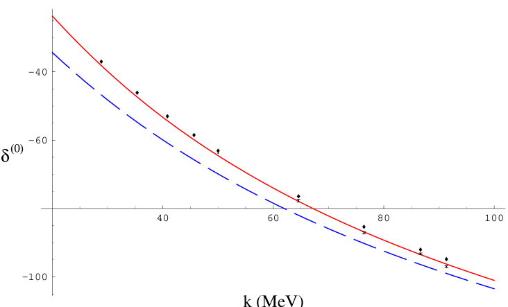
Figure 6: Quartet $S$-wave $N$-$D$ phase shifts $\delta$ in degrees versus center-of-mass momentum $k$ in MeV. Solid curve: EFT $p$-$d$ result; dashed curve: EFT $n$-$d$ result; diamonds: potential model results from Ref. [36] below deuteron breakup and from Ref. [37] above breakup at momentum $k=52.77$ MeV; dots with error bars: TUNL phase shift analysis [38].

One can see some expected pattern from Fig. 6. Coulomb effects are important at low-energies, accounting for as much as $\approx 40\%$ difference between the $n$-$d$ and $p$-$d$ phase shifts at momenta $k\sim 20$ MeV. The $40\%$ effect at $k\sim 20$ is in the Coulomb subtracted phase shift after removing similar sized contributions from the total cross section. It is reasonable to assume that at these low momenta the perturbation has at least a significantly better rate of convergence after the resummation. It would seem that resummation is unnecessary at higher momenta $k\raisebox{-3.01385pt}{$\stackrel{{\scriptstyle\textstyle>}}{{\sim}}$ }60$ MeV where the Coulomb effects in the subtracted phase shift is as low as $6\%$. However, Coulomb effects would still be large in the forward direction in the total cross section. It is also evident that $p$-$d$ phase shift, calculated in EFT, potential model and TUNL phase shift analysis, is consistently larger than the $n$-$d$ phase shifts.

Note that only certain quantities, e.g. conventionally defined $\delta^{l}=\delta^{(l)}_{Full}-\delta^{(l)}_{c}$, have a sensible $\lambda\rightarrow 0$ limit [34]. In order to ensure a sensible $\lambda\rightarrow 0$ limit and to make a meaningful comparison with available partial wave analysis, we use the conventional definition in calculation $\delta^{(l)}$ including resumming Coulomb photons which might not be necessary at large momenta.

The EFT result for $p$-$d$ phase shift agrees with the potential model result and the TUNL phase shift analysis values, within the estimated $\sim 7\%$ theoretical and $\sim 3\%$ numerical error. On closer inspection, it appears that for momenta $p\lesssim 60$ MeV, central value of EFT result is consistently smaller than the TUNL values, whereas for very large momentum $k\sim 100$ MeV it is slightly larger. On the other hand the potential model results are consistently larger by a similar amount.

V Summary

In conclusion, we developed a power counting for the Coulomb effects in the quartet channel for $p$-$d$ systems in a low-energy pionless EFT. The power counting reproduces $p$-$d$ scattering results that have been known in potential models for decades. However, this power counting will be crucial for future EFT three-nucleon calculations beyond the $p$-$d$ elastic scattering process, where precision potential model results might not be available or well known. The quartet channel $S$-wave elastic $p$-$d$ scattering phase shift was calculated both below and above the deuteron breakup threshold. Calculations were performed up to NLO in the Coulomb corrections and N²LO in the strong interactions, with an estimated theoretical error of $\sim 7\%$ and $\sim 3\%$ respectively. An error of about $2\%$ was found in the numerical evaluation of the scattering amplitude. Within the estimated error, the EFT results agree with both potential model calculations and phase shift analysis of experimental data.

The LO and NLO Coulomb ladder contribution is equivalent to contributions from the coordinate space Coulomb potential $V_{c}=\alpha/r$. The large $7\%$ error is primarily from the single photon diagrams, similar to that in Fig. 5(b) dressed with the LO scattering amplitude on the external legs. These diagrams constitute the largest higher order corrections to the Coulomb ladder. There have been some discussion in the literature about Coulomb polarization effects. These effects have been found to be negligible for the present calculation [35] and they are not included.

The power counting for the Coulomb effects developed here could be applied to higher partial waves in both quartet and doublet channel for $p$-$d$ scattering. As mentioned in the introduction, one can then go on to study the so-called $p$-$d$ $A_{y}$ puzzle, and low-energy many-body processes such as $pd\rightarrow\gamma\ ^{3}$He, $dd\rightarrow n\ ^{3}$He, etc., that might be important for placing stricter bound on primordial light element abundances in big-bang nucleosynthesis calculations [26]. Triton beta decay is another important low-energy process where three-body Coulomb effects are important. This process is related to neutrino-deuteron scattering and might have significance to neutrino physics at SNO.

Appendix A The deuteron propagator with Coulomb photon

To understand the power counting rules of Section III, it is most convenient to start with the leading order deuteron propagator, without the range correction:

$$i\Delta(p_{0},{\bm{p}}) = -i\frac{4\pi}{M_{N}y^{2}}\frac{1}{-\gamma+\sqrt{{\bm{p}}^{2}/4-M_{N}p_{0}-i\epsilon}}$$ (19)

$$= -i\frac{4\pi}{M_{N}y^{2}}\frac{\gamma+\sqrt{{\bm{p}}^{2}/4-M_{N}p_{0}}}{{\bm{p}}^{2}/4-M_{N}p_{0}-\gamma^{2}-i\epsilon}\ .$$

In elastic $p$-$d$ scattering, every Feynman diagram with a deuteron propagator involves only a single nucleon propagator at equal times, see Figs. 2,3,4 and 5. The deuteron propagator momentum in any diagram can be written such that $(p_{0}=E_{d}+q_{0},{\bm{p}}={\bm{q}})$ with the corresponding nucleon line carrying energy-momentum $(E_{N}-q_{0},-{\bm{q}})$ where $E_{d}=p^{2}/(4M_{N})-\gamma^{2}/M_{N}$ is the incoming/outgoing deuteron energy and $E_{N}=p^{2}/(2M_{N})$ is the nucleon incoming/outgoing energy with incoming/outgoing momenta $p$, for a generic loop momentum $(q_{0},{\bm{q}})$. We get:

$$i\Delta(E_{d}+q_{0},{\bm{q}}) = -i\frac{4\pi}{M_{N}y^{2}}\frac{\gamma+\sqrt{\frac{{\bm{q}}^{2}-{\bm{p}}^{2}}{4}-M_{N}q_{0}+\gamma^{2}}}{\frac{{\bm{q}}^{2}-{\bm{p}}^{2}}{4}-M_{N}q_{0}-i\epsilon}\ ,$$ (20)

where the factors of $\gamma^{2}$ cancel in the deuteron pole. Carrying out the $q_{0}$ integral, as in Eq. (23), and putting the nucleon on-shell with $q_{0}=E_{N}-{\bm{q}}^{2}/(2M_{N})$ gives

$$i\Delta(E_{d}+E_{N}-\frac{{\bm{q}}^{2}}{2M_{N}},{\bm{q}}) = -i\frac{4\pi}{M_{N}y^{2}}\frac{\gamma+\sqrt{3\frac{{\bm{q}}^{2}-{\bm{p}}^{2}}{4}+\gamma^{2}}}{3\frac{{\bm{q}}^{2}-{\bm{p}}^{2}}{4}}\ .$$ (21)

Including the effective range $\rho$ is straightforward, and we get:

$$i\Delta(E_{d}+E_{N}-\frac{{\bm{q}}^{2}}{2M_{N}},{\bm{q}}) = -i\frac{4\pi}{M_{N}y^{2}}\frac{\gamma+\sqrt{3\frac{{\bm{q}}^{2}-{\bm{p}}^{2}}{4}+\gamma^{2}}}{3\frac{{\bm{q}}^{2}-{\bm{p}}^{2}}{4}}\frac{1}{1-\frac{\rho}{2}\left(\gamma+\sqrt{3\frac{{\bm{q}}^{2}-{\bm{p}}^{2}}{4}+\gamma^{2}}\right)}\ .$$ (22)

We will ignore the effective range corrections $\sim\rho\gamma\sim Q/\Lambda$ in the following discussion for simplicity. For small momenta $p\ll\gamma\sim Q$, when $q\sim p$ ($d^{3}q\sim p^{3}$) we get $\Delta\sim(4\pi)/(M_{N}y^{2})\gamma/p^{2}\sim Q/p^{2}$ whereas when $q\sim\gamma$ ($d^{3}q\sim\gamma^{3}$) we get $\Delta\sim(4\pi)/(M_{N}y^{2}\gamma)\sim 1/Q$. This scaling of the deuteron propagator is far from obvious. Even though one might naively expect $\Delta\sim 1/Q$ from dimensional analysis in Eqs. (5) and (II), this is invalidated since the deuteron can be put on shell which exactly cancels the factors of $\gamma^{2}$ from the deuteron pole.

Now, even though the contribution from the deuteron pole is enhanced for $q\sim p$, its contribution is typically suppressed by $d^{3}q\sim p^{3}$ except when the loop integral also involves a Coulomb photon propagator which scales as $1/q^{2}\sim 1/p^{2}$. This explains why there are no $1/p$ infrared enhancements in the diagrams without photons in Fig. 2, where the dominant contribution comes from loop momentum $q\sim\gamma\sim Q$ with $\Delta\sim 1/Q$. On the other hand diagrams with Coulomb photons get infrared enhancements from $q\sim p$, and $\Delta\sim Q/p^{2}$. For example, from Fig. 3 (f) we get the contribution (ignoring factors of $i$,$2$, $\pi$, etc.,):

$$\sim \int\frac{{\rm d}q_{0}}{2\pi}{\frac{{\rm d}^{3}{\bm{q}}}{(2\pi)^{3}}\,}\Delta(E_{d}+q_{0},{\bm{q}})\frac{1}{-q_{0}+E_{N}-\frac{{\bm{q}}^{2}}{2M_{N}}}\frac{\alpha}{\left({\bm{q}}-{\bm{p}}\right)^{2}}\frac{\alpha}{\left({\bm{q}}-{\bm{k}}\right)^{2}}$$ (23)

$$\sim \int{\frac{{\rm d}^{3}{\bm{q}}}{(2\pi)^{3}}\,}\Delta(E_{d}+E_{n}-\frac{{\bm{q}}^{2}}{2M_{N}},{\bm{q}})\frac{\alpha}{\left({\bm{q}}-{\bm{p}}\right)^{2}}\frac{\alpha}{\left({\bm{q}}-{\bm{k}}\right)^{2}}$$

$$\sim \frac{\alpha^{2}}{My^{2}}\int{\frac{{\rm d}^{3}{\bm{q}}}{(2\pi)^{3}}\,}\frac{(\gamma+\sqrt{3{\bm{q}}^{2}/4-3{\bm{p}}^{2}/4+\gamma^{2}})}{3{\bm{q}}^{2}/4-3{\bm{p}}^{2}/4}\frac{1}{\left({\bm{q}}-{\bm{p}}\right)^{2}}\frac{1}{\left({\bm{q}}^{2}-{\bm{k}}\right)}\ ,$$

where the deuteron energy $E_{d}={\bm{p}}^{2}/(4M_{N})-\gamma^{2}/M_{N}$ and the nucleon energy $E_{N}={\bm{p}}^{2}/(2M_{N})$ with momenta ${\bm{p}}$, ${\bm{k}}$ defined as in Eq. (11). This integral is dominated by momenta $q\sim|p|=|k|$ and the contribution is, without wave function renormalization,

$$\sim \frac{\alpha}{p^{2}}\frac{\alpha Q}{My^{2}p}=\frac{\alpha}{p^{2}}\frac{\alpha M_{N}}{p}\times\frac{Q}{M_{N}^{2}y^{2}}\ .$$ (24)

Diagrams without a deuteron propagator involve three nucleons. After carrying out the integral over the energy component $q_{0}$ and putting a nucleon on-shell, one is left with two nucleons that are always regulated in the infra red by the deuteron binding momentum $\gamma$, as these involve two nucleons that carry the energy $E_{d}$ of the “parent” deuteron. For example, in Fig. 3 (b) we have

$$\sim y^{2}\int\frac{{\rm d}q_{0}}{2\pi}{\frac{{\rm d}^{3}{\bm{q}}}{(2\pi)^{3}}\,}\frac{1}{-q_{0}-\frac{{\bm{q}}^{2}}{2M_{N}}}\frac{1}{q_{0}+E_{d}-\frac{({\bm{q}}+{\bm{p}})^{2}}{2M_{N}}}\frac{1}{q_{0}+E_{d}-\frac{({\bm{q}}+{\bm{k}})^{2}}{2M_{N}}}\frac{\alpha}{({\bm{p}}-{\bm{k}})^{2}}$$ (25)

$$\sim \frac{\alpha y^{2}M_{N}^{2}}{({\bm{p}}-{\bm{k}})^{2}}\int{\frac{{\rm d}^{3}{\bm{q}}}{(2\pi)^{3}}\,}\frac{1}{\frac{({\bm{q}}+{\bm{p}})^{2}}{2}+\frac{{\bm{q}}^{2}}{2}-\frac{{\bm{p}}^{2}}{2}+\gamma^{2}}\frac{1}{\frac{({\bm{q}}+{\bm{k}})^{2}}{2}+\frac{{\bm{q}}^{2}}{2}-\frac{{\bm{p}}^{2}}{2}+\gamma^{2}}$$

$$\sim \frac{\alpha y^{2}M_{N}^{2}}{{\bm{p}}^{2}Q}\ ,$$

where the nucleon propagators get regulated in the infrared by the deuteron binding momentum $\gamma\sim Q$ with $|{\bm{p}}|=|{\bm{k}}|$. After wave function renormalization $Z_{d}\sim Q/(M_{N}^{2}y^{2})$, it gives a contribution $\sim\alpha/p^{2}$. Exact evaluation of the integral gives

$$\frac{1}{2\pi({\bm{p}}-{\bm{k}})^{2}}\arctan\left[\frac{1}{2}\sqrt{\frac{({\bm{p}}-{\bm{k}})^{2}}{4\gamma^{2}-{\bm{p}}^{2}}}\right]\sim\frac{1}{8\pi\gamma}+{\mathcal{O}}(p^{2}),$$ (26)

which is consistent with the power counting estimate (including all the numerical factors).

To summarize, all the nucleon propagators scale as $M_{N}/Q^{2}$, the deuteron propagator scales as $Q/q^{2}$ and the Coulomb photon propagators scale as $1/q^{2}$. The loop momentum scales as either $q\sim p\ll Q$ or as $q\sim Q$, and correspondingly the deuteron propagator scales as $1/Q$ or $Q/p^{2}$. In estimating the dominant contributions from a loop integral for $q\sim p$, one has to consider the suppression factors from $d^{3}q\sim p^{3}$ along with infrared enhancements from the deuteron $Q/p^{2}$ and the photons $1/p^{2}$.

References

- [1] Proceedings in Nuclear Physics with Effective Field Theory edited by R. Seki, U. van Kolck and M.J. Savage (World Scientific, Singapore, 1998, ISBN 981-02-3596-8) and Nuclear Physics with Effective Field Theory II edited by P. F. Bedaque, M. J. Savage, R. Seki and U. van Kolck (World Scientific, Singapore, 1999, ISBN 981-02-4181-X).
- [2] S.R. Beane, P.F. Bedaque, W.C. Haxton, D.R. Phillips and M.J. Savage, “From Hadrons to Nuclei: Crossing the Border”, essay for the Festschrift in honour of Boris Ioffe, to be published as ’Encyclopedia of Analytic QCD’, ed. M. Shifman, World Scientific, nucl-th/0008064.
- [3] S. Weinberg, Phys. Lett. B 251, 288 (1990); Nucl. Phys. B 363, 3 (1991); Phys. Lett. B 295, 114 (1992).
- [4] C. Ordonez and U. van Kolck, Phys. Lett. B 291, 459 (1992); C. Ordonez, L. Ray and U. van Kolck, Phys. Rev. Lett. 72, 1982 (1994); Phys. Rev. C 53, 2086 (1996); U. van Kolck, Phys. Rev. C 49, 2932 (1994).
- [5] T. Mehen and I. W. Stewart, Phys. Lett. B 445, 378 (1999); Phys. Rev. C 59, 2365 (1999).
- [6] G. Rupak and N. Shoresh, Phys. Rev. C 60, 054004 (1999); nucl-th/9906077 in Nuclear Physics with Effective Field Theory II edited by P. F. Bedaque, M. J. Savage, R. Seki and U. van Kolck (World Scientific, Singapore, 1999, ISBN 981-02-4181-X).
- [7] T. D. Cohen and J. M. Hansen, Phys. Rev. C 59, 13 (1999); Phys. Rev. C 59, 3047 (1999); nucl-th/9908049.
- [8] S. Fleming, T. Mehen and I. S. Stewart, Phys. Rev. C 61, 044005 (2000).
- [9] E. Epelbaoum and U.G. Meissner, Phys. Lett. B 461, 287 (1999); E. Epelbaoum, W. Glockle, A. Kruger and Ulf-G. Meissner, Nucl. Phys. A 645, 413 (1999); E. Epelbaoum, W. Glockle and Ulf-G. Meissner, Phys. Lett. B 439, 1 (1998); E. Epelbaoum, W. Glockle and Ulf-G. Meissner, Nucl. Phys. A 637, 107 (1998); U.G. Meissner, E. Epelbaum and W. Glockle, Nucl. Phys. A 684, 371 (2001).
- [10] U. van Kolck, hep-ph/9711222, in Nuclear Physics with Effective Field Theory edited by R. Seki, U. van Kolck and M.J. Savage (World Scientific, Singapore, 1998, ISBN 981-02-3596-8), Nucl. Phys. A 645, 273 (1999).
- [11] P.F. Bedaque, H.W. Hammer and U. van Kolck, Nucl. Phys. A 676, 357 (2000); Nucl. Phys. A 646, 444 (1999); Phys. Rev. Lett. 82, 463 (1999); Phys. Rev. C 58, R641 (1998); P.F. Bedaque and U. van Kolck, Phys. Lett. B 428, 221 (1998).
- [12] J. Gegelia, nucl-th/9802038, contributed to Workshop on Methods of Nonperturbative Quantum Field Theory, Adelaide, Australia, 2-13 Feb 1998.
- [13] J.W. Chen, G. Rupak and M.J. Savage, Nucl. Phys. A 653, 386 (1999).
- [14] J.W. Chen, G. Rupak and M.J. Savage, Phys. Lett. B 464, 1 (1999).
- [15] M. N. Butler and J. W. Chen, nucl-th/0101017.
- [16] M. N. Butler, J. W. Chen and X. Kong, Phys. Rev. C 63, 035501 (2001).
- [17] X. Kong and F. Ravndal, Nucl. Phys. A 665, 137 (2000); Nucl. Phys. A 656, 421 (1999); Phys. Lett. B 470, 1 (1999); Phys. Lett. B 450, 320 (1999).
- [18] X. Kong and F. Ravndal, nucl-th/0004038.
- [19] G. Rupak, Nucl. Phys. A 678, 405 (2000).
- [20] H.W. Grießhammer and G. Rupak, nucl-th/0012096.
- [21] P.F. Bedaque and H.W. Grießhammer, Nucl. Phys. A 671, 357 (2000).
- [22] F. Gabbiani, P.F. Bedaque and H.W. Grießhammer, Nucl. Phys. A 675, 601 (2000).
- [23] F. Gabbiani, nucl-th/0104088
- [24] H. W. Hammer and T. Mehen, nucl-th/0105072.
- [25] P. F. Bedaque, G. Rupak, H. W. Griesshammer and H. W. Hammer, nucl-th/0207034.
- [26] S. Burles, K.M. Nollet, J.N. Truran and M.S. Turner, Phys. Rev. Lett. 82, 4176 (1999).
- [27] R. Schiavilla et. al., Phys. Rev. C 58, 1263 (1998).
- [28] D.B. Kaplan, M.J. Savage and M.B. Wise, Phys. Lett. B 424, 390 (1998), Nucl. Phys. B 534, 329 (1998).
- [29] D. B. Kaplan, Nucl. Phys. B 494, 471 (1997)
- [30] S.R. Beane and M.J. Savege, nucl-th/0011067.
- [31] C. van der Leun and C. Anderliesten, Nucl. Phys. A 380, 261 (1982).
- [32] V.G.J. Stoks, R.A.M. Klomp, M.C.M. Rentmeester and J.J. de Swart, Phys. Rev. C 48, 792 (1993). V.G.J. Stoks, R.A.M. Klomp, C.P.F. Terheggen and J.J. de Swart, Phys. Rev. C 49, 2950 (1994).
- [33] J.L. Friar and G.L. Payne in Coulomb Interactions in Nuclear and Atomic Few-Body Collisions pg. 97-168 edited by F.S. Levin and D.A. Micha (Plenum Press, New York, 1996, ISBN 0-306-45149-2).
- [34] E.O. Alt, W. Sandhas and H. Ziegelmann, Nucl. Phys. A 445, 429 (1985); E.O. Alt and W. Sandhas in Coulomb Interactions in Nuclear and Atomic Few-Body Collisions pg. 1-95 edited by F.S. Levin and D.A. Micha (Plenum Press, New York, 1996, ISBN 0-306-45149-2).
- [35] G.H. Berthold and H. Zankel, Phys. Rev. C 4, 34 (1986).
- [36] A. Kievsky et. al., Nucl. Phys. A 607, 402 (1996).
- [37] W. Tornow, Private communication: Phase shift above deuteron breakup momentum MeV from potential model AV18.
- [38] W. Tornow, Private communication: Phase shift analysis from TUNL.