Hadron structure and the limitations of phenomenological models in electromagnetic reactions

Abstract

The description of electromagnetic reactions at intermediate energies, such as pion electroproduction or (virtual) Compton scattering, traditionally starts from covariant tree-level Feynman diagrams (Born or pole terms). Internal hadron structure is included by means of (on-shell) form factors in the vertices while free propagators are used. To overcome problems with gauge invariance, simple prescriptions such as choosing $F_{1}^{V}(q^{2})=F_{\pi}(q^{2})$ in pion electroproduction or the “minimal substitution” are used. We discuss the limitations of such approaches by comparing to the most general structure of electromagnetic vertices and propagators for pions and nucleons. The recipes to enforce gauge invariance are critically examined and contrasted with the exact treatment. The interplay between off-shell effects and irreducible “contact” terms is demonstrated for real Compton scattering on a pion. The need for a consistent microscopic treatment of reaction amplitudes is stressed. Shortcomings of minimal substitution are illustrated through an example in the framework of chiral perturbation theory.

I Introduction

High-precision experiments at intermediate energies with electromagnetic probes are presently being carried out with the goal to investigate the internal structure of the participating hadrons and to probe details of the reaction dynamics. A recent example is the measurement of pion electroproduction on the nucleon to determine the axial and electromagnetic form factors of the nucleon and the pion, respectively [1, 2]. In this paper we will point out some of the limitations and shortcomings in the commonly used phenomenological approaches to describe these reactions and show how in contrast structure and dynamics are addressed consistently in microscopic approaches such as chiral perturbation theory.

Most theoretical descriptions of intermediate-energy reactions, such as Compton scattering or pion electroproduction on a nucleon, have dealt with internal hadron structure and the reaction dynamics in a more global fashion and not used a microscopic model for these aspects. Instead, a description based on covariant tree-level Feynman diagrams (Born or pole terms) has been used, where the free hadron properties are the building blocks. The limitations of this approach are immediately obvious from this simple observation: these reactions necessarily involve intermediate particles that are not free, i.e. are “off mass shell.” For example, two-step processes on the nucleon, such as Compton scattering, necessarily involve off-shell nucleons; in pion photo- or electroproduction on the nucleon, in addition, there is an off-shell pion.

This fact implies that for the interpretation of these reactions we need more input than just the free, on-shell properties of the participating particles. It adds complexity to the theoretical description: the general structure of the electromagnetic vertex of a given hadron, for example, is more complicated and the associated form factors will depend on more scalar variables than in the free case [3, 4, 5]. Nevertheless, encouraged by theorems which express reaction amplitudes in certain low-energy limits in terms of on-shell properties of the participating particles, it has been customary for decades to describe two-step processes on e.g. nucleons also at intermediate energies in terms of simple “Born amplitudes,” which only involve on-shell information in vertices and propagators.

Interestingly enough, the articles deriving these low-energy theorems [6, 7] were the first to point out the more complex structure of vertices and propagators in the general case at higher energies. What they also emphasized was that the internal structure of the hadrons necessarily leads to new classes of amplitudes. For example, a diagram that in a given model contributes to the electromagnetic structure of a nucleon, will give rise to irreducible two-photon amplitudes for Compton scattering (see Fig. 1). However, these aspects are absent in the widely used Born-term description of Compton scattering or pion photo- and electroproduction.

An objective indication that some important physics is missing in the usual theoretical approaches is provided by gauge invariance. When form factors are included in the Born terms, one typically obtains amplitudes that are not gauge invariant. Even though the cause of this problem can be understood and addressed when one consistently deals with the origin of the internal structure, most authors reverted to a variety of ad hoc recipes to restore gauge invariance in Born-type amplitudes: terms are added by hand or form factors are adjusted to yield a conserved current. In pion electroproduction, for example, a commonly made assumption for this purpose is that the pion and nucleon isovector form factors are identical [8, 9, 10]. Similary, both the pion-pole term and the nucleon-pole term, which is needed for gauge invariance, are proportional to the pion form factor in the model [11, 12] used to analyze the data in Ref. [2]. These assumptions may very well limit the use of this model for extracting the pion form factor from experiment.

Another way to deal with this problem are the extended Born terms by Haberzettl et al. [13]. They include off-shell modifications at the hadron vertices in pion photoproduction, consistent with current conservation. This approach (which has recently been shown to violate crossing symmetry in its original form [14]) can, through its additional free parameters, lead to an improved phenomenology. However, without a (field-theoretical) microscopic basis it is unclear how it can be used to reliably extract information about hadron structure. As has been stressed in Refs. [15, 16, 17, 18], off-shell properties of particles are not observables. They are not unique, depending not only on the microscopic model, but also on the representation one chooses for the interpolating fields of the (intermediate) particles [15, 16, 17, 18]. In some cases, they can completely be transformed into reaction-specific contact terms. When we talk below about “off-shell effects” this caveat should be kept in mind.

A direct way to preserve gauge invariance for phenomenological models is the minimal substitution. It couples a photon to a given charged system, generating a restricted or “minimal” set of terms which guarantee a gauge-invariant amplitude. This prescription has been critically reviewed in Ref. [19]. It has mainly been applied in pion photoproduction [20], where the use of a strong pion-nucleon form factor leads in general to a photoproduction amplitude that is not gauge invariant. The importance of the terms one misses by using this prescription has been illustrated in Ref. [21] in the context of a simple model for pion photo- and electroproduction.

In this paper we address these general questions related to the internal hadron structure in electromagnetic reactions and to gauge invariance. We use the pion as the main example, since the formalism remains simple in comparison to the nucleon or particles with higher spin, while all important aspects can be studied. We start in Sec. II with a discussion of the features of the general pion electromagnetic vertex. Many of them have been known for decades [22, 23, 24], but have largely been ignored in theoretical descriptions of modern experiments. We examine to what extent this vertex can be obtained through minimal substitution into the pion self energy for real and virtual photons. We then extend the discussion to the electromagnetic vertex of the nucleon. In Sec. III we investigate Compton scattering off a pion as a protoptype for a two-step process. Special attention is paid to the question how “off-shell effects” can contribute to the amplitude. We then contrast the general Compton scattering amplitude for a pion with the amplitude generated through minimal substitution.

Clearly the most sensible way to address the physics of hadron structure and reaction mechanism in a consistent fashion, while avoiding the complications and recipes mentioned above, is to work in the framework of a well-defined (effective) field theory, such as chiral perturbation theory (ChPT). In Sec. IV we illustrate this by looking at the pion electromagnetic form factor to one loop in the framework of ChPT and investigate if the minimal substitution recipe can be applied on the level of the Lagrangian itself. General conclusions are presented in Sec. V.

II Electromagnetic Vertex of Composite Particles: General Features, the Minimal Substitution and other recipes

In this section we discuss the most general structure of the electromagnetic vertex of spin-$0$ and spin-$\frac{1}{2}$ particles and contrast it with the vertex of the free particles. We show what restrictions the Ward-Takahashi (WT) identity [25, 26] imposes and stress how a consistent treatment of propagator and vertex structure makes it unnecessary to interrelate pion and nucleon form factors as is commonly done. Finally, we discuss to what extent the minimal substitution generates the off-shell vertices needed for the description of the electromagnetic interaction with intermediate particles.

A General features of the pion electromagnetic vertex

For a spin-$0$ particle (we will for simplicity focus on a charged pion) Lorentz invariance restricts the form of the electromagnetic vertex operator to

$${\it\Gamma}^{\mu}(p\,^{\prime},p)=e\,\left[(p\,^{\prime}+p)^{\mu}F(q^{2},p\,^{\prime 2},p^{2})+\ q^{\mu}\,G(q^{2},p\,^{\prime 2},p^{2})\right]\;,$$ (1)

where $p$ and $p\,^{\prime}$ are the initial and final momenta of the meson, respectively, and the photon momentum is

$$q=p\,^{\prime}-p\;.$$ (2)

The neutral pion is its own antiparticle and, because of $C$ invariance, has no electromagnetic form factor even off shell. The functions $F$ and $G$ are form factors which in general depend on three scalar variables. For simplicity we do not indicate if a form factor refers to a positive or negative pion. Time-reversal invariance imposes further constraints on the functions $F$ and $G$,

$$F(q^{2},p\,^{\prime 2},p^{2})=F(q^{2},p^{2},p\,^{\prime 2}),\quad G(q^{2},p\,^{\prime 2},p^{2})=-G(q^{2},p^{2},p\,^{\prime 2})\;,$$ (3)

whereas from Hermiticity follows, for $q^{2}\leq 0$,

$$F(q^{2},m^{2},m^{2})=F^{\ast}(q^{2},m^{2},m^{2})\;.$$ (4)

Assuming that we are dealing with the irreducible electromagnetic vertex operator, the requirement of gauge invariance yields the WT identity:

$$q_{\mu}{\it\Gamma}^{\mu}(p\,^{\prime},p)=e_{\pi}\left[\,\Delta^{-1}(p\,^{\prime})-\Delta^{-1}(p)\,\right]\;,$$ (5)

where $\Delta(p)$ denotes the dressed, renormalized propagator of the meson and $e_{\pi}=e\,\hat{e}_{\pi}$ ($\hat{e}_{\pi^{\pm}}=\pm 1$). Using the general form in Eq. (1), the WT identity becomes

$$(p\,^{\prime 2}-p^{2})\;F(q^{2},p\,^{\prime 2},p^{2})+q^{2}\;G(q^{2},p\,^{\prime 2},p^{2})=\hat{e}_{\pi}\left[\Delta^{-1}(p\,^{\prime})-\Delta^{-1}(p)\right]\;,$$ (6)

providing a relation between the functions $F$ and $G$ and the propagator $\Delta$ of the meson. From Eq. (3) or the WT identity it can be easily seen that

$$G(q^{2},p^{2},p^{2})=0\;,$$ (7)

i.e. this function vanishes when the invariant masses of the initial and final meson are equal. This implies that $G$ can be written as

$$G(q^{2},p\,^{\prime 2},p^{2})=(p\,^{\prime 2}-p^{2})\;g(q^{2},p\,^{\prime 2},p^{2})\;,$$ (8)

where the function $g$ is nonsingular at $p\,^{\prime 2}=p^{2}$.

It is instructive to use the above result to rewrite the general electromagnetic vertex of the scalar particle as

$${\it\Gamma}^{\mu}(p\,^{\prime},p)=e\,\left[(p\,^{\prime}+p)^{\mu}f(p\,^{\prime 2},p^{2})+\left(q^{\mu}q^{\nu}-g^{\mu\nu}q^{2}\right)(p\,^{\prime}+p)_{\nu}\;g(q^{2},p\,^{\prime 2},p^{2})\right]\;,$$ (9)

where $f$ is defined as

$$f(p\,^{\prime 2},p^{2}) = F(q^{2},p\,^{\prime 2},p^{2})+\frac{q^{2}}{p\,^{\prime 2}-p^{2}}G(q^{2},p\,^{\prime 2},p^{2})$$ (10)

$$= F(q^{2},p\,^{\prime 2},p^{2})+q^{2}\,g(q^{2},p\,^{\prime 2},p^{2})\;.$$ (11)

By contracting Eq. (9) with $q_{\mu}$, we see that the function $f$ is entirely determined through the WT identity and depends only on two scalar variables, the invariant masses $p\,^{\prime 2}$ and $p^{2}$,

$$f(p\,^{\prime 2},p^{2})=\hat{e}_{\pi}\frac{\Delta^{-1}(p\,^{\prime})-\Delta^{-1}(p)}{p\,^{\prime 2}-p^{2}}\;.$$ (12)

The second term in Eq. (9) is separately gauge invariant and no gauge constraints exist for the function $g(q^{2},p\,^{\prime 2},p^{2})$. Only due the presence of this term does the vertex depend on $q^{2}$. In the framework of an effective Lagrangian, such a term can be understood in terms of the gauge-invariant combination

$$F_{\mu\nu}=-i(q_{\mu}\epsilon_{\nu}-q_{\nu}\epsilon_{\mu}),$$ (13)

representing the Fourier component of the electromagnetic field strength tensor ${\cal F}_{\mu\nu}(x)=\partial_{\mu}A_{\nu}(x)-\partial_{\nu}A_{\mu}(x)$ associated with a plane-wave (virtual) photon $A_{\mu}(x)=\epsilon_{\mu}\exp(-iq\cdot x)$. In a reaction amplitude, the structure multiplying the function $g$ then results from the contraction of $q_{\mu}F^{\mu\nu}$ with the sum of the pion momenta $(p\,^{\prime}+p)_{\nu}$. Thus, for the pion, such a separately gauge-invariant term is at least of second order in the photon four-momentum. Furthermore, powers of $q^{2}$, $p\,^{\prime 2}$, and $p^{2}$ in $g(q^{2},p\,^{\prime 2},p^{2})$ can be thought of as originating in powers of (covariant) derivatives acting on the field-strength tensor, and the final and initial charged-particle fields, respectively.

The fact that the function $G(q^{2},p\,^{\prime 2},p^{2})$—or $g(q^{2},p\,^{\prime 2},p^{2})$—is crucial for the $q^{2}$ dependence can already be seen by looking at the WT identity. The right-hand side of Eq. (6) depends only on $p^{2}$ and $p\,^{\prime 2}$, but not on $q^{2}$. Hence without the term involving $G$, the form factor $F$ (and with it the entire vertex) could not depend on $q^{2}$ [23]!

However, it should be stressed that the vanishing of $G(q^{2},p\,^{\prime 2},p^{2})$ for $p\,^{\prime 2}=p^{2}$ according to Eq. (7) does not rule out a $q^{2}$ dependence of the vertex, since in that limit

$$\lim_{p\,^{\prime 2}\rightarrow p^{2}}{\it\Gamma}^{\mu}(p\,^{\prime},p)=e\,(p+p\,^{\prime})^{\mu}F(q^{2},p^{2},p^{2})\;,$$ (14)

and we have from the WT identity, Eq. (6), and Eq. (8),

$$F(q^{2},p^{2},p^{2})=\hat{e}_{\pi}\frac{\partial\Delta^{-1}(p)}{\partial p^{2}}-q^{2}g(q^{2},p^{2},p^{2})\;.$$ (15)

This includes of course the on-shell case, $p^{2}=p\,^{\prime 2}=m^{2}$, which is characterized by a single on-shell form factor

$$F(q^{2})\equiv\left.F(q^{2},p^{2},p^{2})\right|_{p^{2}=m^{2}}\;.$$ (16)

The significance of the second term in Eq. (1) is not clearly recognized in much of the literature. This term is often dropped right from the start. The reason given for ignoring it is that a term in the vertex proportional to $q_{\mu}$ will not contribute for virtual photons originating from a conserved current. However, this argument only works in a covariant gauge, e.g. in the Feynman or Landau gauge [27, 28]. In noncovariant gauges, such as the Coulomb gauge, the gauge term proportional to $q_{\mu}$ must not be neglected since one otherwise would not arrive at the same physical amplitude as in other gauges. By dropping this term in the vertex, one gives away the possibility to freely choose a convenient gauge.

For the interaction of a pion with a real photon, the term proportional to $q_{\mu}$ can be ignored when calculating an amplitude since $\epsilon\cdot q=0$. Since $q^{2}=0$, one only needs

$${\it\Gamma}^{\mu}_{q^{2}=0}(p\,^{\prime},p) = e\,(p\,^{\prime}+p)^{\mu}f(p\,^{\prime 2},p^{2})$$ (17)

$$= e\,(p\,^{\prime}+p)^{\mu}F(0,p\,^{\prime 2},p^{2})$$ (18)

$$= e_{\pi}(p\,^{\prime}+p)^{\mu}\,\frac{\Delta^{-1}(p\,^{\prime})-\Delta^{-1}(p)}{p\,^{\prime 2}-p^{2}}\;.$$ (19)

Thus by using Lorentz symmetry and gauge invariance, the electromagnetic vertex needed for real photons can be shown to be entirely determined in terms of the finite derivative of the inverse meson propagator. This includes the dependence of the vertex on the off-shell variables $p^{2}$ and $p\,^{\prime 2}$. The situation is entirely different for virtual photons. The function $F$ depends on $q^{2}$ as well and the term involving $G$ must in general be kept.

B The pion form factor in pion electroproduction

We now address the question of form factors in pion electroproduction on the nucleon. In the usual description based on pole terms or Born diagrams, the pion-pole term is the only term where the electromagnetic form factor of the pion appears. Since this term is not separately gauge invariant, gauge invariance of the total amplitude is achieved through cancellation with other terms. To make this cancellation with other diagrams, which involve nucleon form factors, possible, one is forced to make assumptions about these form factors, namely

$$F_{1}^{V}(q^{2})=F_{\pi}(q^{2})\;,$$ (20)

where $F_{1}^{V}$ is the electromagnetic isovector form factor of the nucleon. In a similar vein, both the reggeized pion-pole term and the nucleon-pole term were described through the same form factor, $F_{\pi}$, to insure gauge invariance in Refs. [11, 12], which was the basis for the form factor determination of Ref. [2]. Clearly such assumptions, which are commonly made (see, e.g., Refs. [9, 10])—unless they can be put on a firm physical basis—should be avoided when extracting detailed information such as a pion form factor from electroproduction experiments.

In contrast, a description that consistently uses a dressed pion propagator and vertex in agreement with the WT identity does not have to make this assumption. The intermediate pion in the pion-pole term is half off shell (see Fig. 2). When one tests gauge invariance and contracts the pion-pole term with the photon momentum, it is then easily seen from Eq. (5) that, with $p\,^{\prime 2}=m^{2}$ and $\tilde{p}$ the momentum of the intermediate pion, one obtains

$$q_{\mu}\,\Gamma^{\mu}(p\,^{\prime},{\tilde{p}})\,\Delta({\tilde{p}}) = e_{\pi}\left[\Delta^{-1}(p^{\prime})-\Delta^{-1}({\tilde{p}})\right]\,\Delta({\tilde{p}})$$ (21)

$$= -\,e_{\pi}\;.$$ (22)

The divergence of the pion-pole term, where internal structure is consistently included in pion vertex and propagator, is thus independent of any detailed pion properties. Analogous statements hold for the nucleon-pole terms and the mutual cancellation of pion- and nucleon-pole terms is obtained without any assumptions about the different form factors. What the WT identity obviously tells us is that we must simultaneously and consistently deal with both the electromagnetic vertex and the propagator of the same hadron to arrive at a gauge-invariant description. (Of course, the pion-pole term is also the only term involving the strong $\pi NN$ form factor for an off-shell pion. We refer to, e.g., Refs. [22, 29] for a discussion how to deal consistently with this aspect).

In principle, there is one particular representation, the “canonical” form, where it is possible to work with free electromagnetic form factors and propagators. However, the price one pays for this is the presence of a number of irreducible “contact” terms specific for the reaction under study. While this representation is convenient for general purposes such as the derivation of low-energy theorems for (virtual) Compton scattering [30, 31], it has little use in practical applications. Furthermore, the possibility to move off-shell effects into contact terms makes assumptions about the analyticity of the amplitude. Above production thresholds one will therefore face difficulties in this respect [15].

C The minimal-substitution vertex

We now compare the general vertex discussed above with the vertex one gets by minimal substitution, $\Gamma^{\mu}_{\rm MS}$. An extensive review of the minimal substitution can be found in Ref. [32] and we here only briefly outline the procedure. It is obtained by making the “substitution” $p\rightarrow p-e_{\pi}\,A$ in $-\Delta^{-1}(p)$ and then identifying—in general, via a functional derivative—the term linear in $A_{\mu}$. This is most easily done by expanding the inverse propagator around $p^{2}=m^{2}$, i.e.

$$\Delta^{-1}(p)=\sum\limits_{n=0}^{\infty}c_{n}(p^{2}-m^{2})^{n},\,\,\,\,\,c_{n}=\left.\frac{1}{n!}(\partial/\partial p^{2})^{n}\,\Delta^{-1}(p)\right|_{p^{2}=m^{2}}.$$ (23)

The validity of this expansion is implied by the applicability of the renormalization procedure; in the on-shell renormalization scheme one has $c_{0}=0,\,c_{1}=1$. In performing the above substitution, we have to keep in mind that $p_{\mu}$ and the electromagnetic field, $A_{\mu}$, do not commute. One obtains from the term linear in $A_{\mu}$ the minimal-substitution vertex

$${{\it\Gamma}}^{\mu}_{\rm MS}(p\,^{\prime},p)=e_{\pi}(p\,^{\prime}+p)^{\mu}\sum_{n=1}^{\infty}c_{n}\sum\limits_{l=1}^{n}(p\,^{\prime 2}-m^{2})^{l-1}\,(p^{2}-m^{2})^{n-l}\;.$$ (24)

Using the identity

$$a^{n}-b^{n}=(a-b)\sum\limits_{l=1}^{n}a^{n-l}\,b^{l-1}$$

we can rewrite the result in terms of the finite-difference derivative of the inverse propagator:

$${{\it\Gamma}}^{\mu}_{\rm MS}(p\,^{\prime},p) = e_{\pi}(p\,^{\prime}+p)^{\mu}\,\frac{\Delta^{-1}(p\,^{\prime})-\Delta^{-1}(p)}{p\,^{\prime 2}-p^{2}}$$ (25)

$$= e_{\pi}(p\,^{\prime}+p)^{\mu}f(p\,^{\prime 2},p^{2}).$$ (26)

By comparing to the general form in Eq. (9), one sees that the minimal-substitution vertex differs in two respects: its operator structure and the dependence on scalar variables. Minimal substitution generates the first term $\sim(p\,^{\prime}+p)^{\mu}$, which depends only on $p\,^{\prime 2}$ and $p^{2}$. It does not produce the second, separately gauge-invariant term, which is crucial for having a vertex that depends on the scalar variable $q^{2}$. In the following we will refer to this second term as “non-minimal” in distinction of the minimal term of Eq. (26). The minimal-substitution recipe, while producing a vertex in general compliance with the WT identity, clearly leads to an unsatisfactory result for virtual photons.

However, the vertex obtained from minimal substitution into the self-energy is precisely the off-shell vertex needed for a real photon, ${{\it\Gamma}}^{\mu}_{{\rm MS},q^{2}=0}$ in Eq. (19),

$${{\it\Gamma}}^{\mu}_{\rm MS}(p\,^{\prime},p)={\it\Gamma}^{\mu}_{q^{2}=0}(p\,^{\prime},p)\;.$$ (27)

Thus for the interaction of a real photon with a pion, the result of minimal substitution into the self energy and of a microscopic Lorentz- and gauge-invariant calculation are identical, as long as the underlying dynamics is dealt with consistently in the calculation of both the vertex and the self energy, e.g. both are calculated to the same order in an expansion parameter. However, this finding at $q^{2}=0$, where minimal substitution leads to the same answer as a microscopic calculation, is an exception. It is due to the fact that for a scalar particle the WT identity completely specifies the vertex needed for the interaction with a real photon. For $q^{2}\neq 0$ the minimal substitution makes little sense, since it does not yield a vertex that depends on the scalar variable $q^{2}$. To obtain such a dependence we would need a “non-minimal” term involving the function $g$, which minimal substitution does not generate.

D Electromagnetic vertex of the nucleon

In concluding this section, we point out that similar considerations also apply to particles with spin 1/2, such as the nucleon [3, 4, 22].

The general electromagnetic vertex operator is commonly written in the form [3]

$$\Gamma^{\mu}(p\,^{\prime},p)=e\sum_{i,j=+,-}\Lambda_{i}(p\,^{\prime})\left[\gamma^{\mu}F_{ij}^{1}+i\frac{\sigma^{\mu\nu}q_{\nu}}{2M}\,F_{ij}^{2}+\frac{q^{\mu}}{M}F_{ij}^{3}\right]\Lambda_{j}(p)\;,$$ (28)

where the $F_{ij}^{1,2,3}$—the twelve form factors that characterize the off-shell vertex—are scalar functions of $q^{2}$, ${p\,^{\prime}}^{2}$, and $p^{2}$, and we have used the projection operators

$$\Lambda_{\pm}(p)=\frac{W\pm p\!\!\!/}{2W}\;,\;\;W=\sqrt{p^{2}}\;.$$ (29)

For simplicity we do not show a charge (or isospin) index. To stay close to the discussion of the pion vertex, we choose here an alternative form [33],

$$\Gamma^{\mu}(p\,^{\prime},p)=e\left(1-\frac{q^{2}}{4M^{2}}\right)^{-1}\,\sum_{i,j=+,-}\Lambda_{i}(p\,^{\prime})\left(\frac{P^{\mu}}{M}\,G_{ij}^{E}+N^{\mu}\,G_{ij}^{M}+\frac{q^{\mu}}{2M}\,G_{ij}^{q}\right)\Lambda_{j}(p)\;,$$ (30)

where

$$N^{\mu}=\frac{\gamma^{\mu}\,P\!\!\!/\,q\!\!\!/-q\!\!\!/\,P\!\!\!/\,\gamma^{\mu}}{4M^{2}}\;,\;\;P=\frac{p\,^{\prime}+p}{2}\;.$$ (31)

Note that $N^{\mu}$ satisfies

$$q\cdot N=0\;.$$ (32)

Just as for the pion, the functions multiplying the term proportional to $q^{\mu}$ must vanish for $p^{2}=p\,^{\prime 2}$ and it is convenient to introduce [cf. Eq. (8)]

$$G_{ij}^{q}(q^{2},p\,^{\prime 2},p^{2})=(p\,^{\prime 2}-p^{2})\;g_{ij}^{q}(q^{2},p\,^{\prime 2},p^{2})\;.$$ (33)

With this property, it is easily seen that the on-shell matrix element of Eq. (30) yields the well-known parametrization of the free current involving the Sachs form factors $G_{E}$ and $G_{M}$.

Further restrictions for the vertex arise from the WT identity,

$$q_{\mu}\,\Gamma^{\mu}(p\,^{\prime},p)=e_{N}\,[S^{-1}(p\,^{\prime})-S^{-1}(p)]\;,$$ (34)

where $e_{N}=e\,{\hat{e}}_{N}$ is the charge of the nucleon (${\hat{e}}_{p}=1,\,{\hat{e}}_{n}=0$) and $S^{-1}$ is the inverse propagator of the nucleon, which we parametrize as

$$S^{-1}(p)=A(p^{2})+\frac{p\!\!\!/}{W}\,B(p^{2})\;.$$ (35)

Projecting out terms in the WT identity by using the projection operators $\Lambda_{\pm}$, we obtain [27]

$$G_{ij}^{E}(q^{2},p\,^{\prime 2},p^{2})+{q^{2}}\,g^{q}_{ij}(q^{2},p\,^{\prime 2},p^{2})=$$ (37)

$$\frac{2M}{p\,^{\prime 2}-p^{2}}\left(1-\frac{q^{2}}{4M^{2}}\right){\hat{e}}_{N}\left[A(p\,^{\prime 2})-A(p^{2})+iB(p\,^{\prime 2})-jB(p^{2})\right].$$

We see that for a real photon the four off-shell functions $G^{E}_{\pm\pm}(0,p\,^{\prime 2},p^{2})$ can be expressed through properties of the nucleon propagator. Using the above equation to eliminate $G^{E}_{ij}$, the covariant nucleon vertex which satisfies the WT identity can be written, in general, in a form similar to Eq. (9),

$$\Gamma^{\mu}(p\,^{\prime},p) = e_{N}\,(p\,^{\prime}+p)^{\mu}\;\frac{S^{-1}(p\,^{\prime})-S^{-1}(p)}{p\,^{\prime 2}-p^{2}}+e\,\left(1-\frac{q^{2}}{4M^{2}}\right)^{-1}$$ (39)

$$\times\sum_{i,j=+,-}\Lambda_{i}(p\,^{\prime})\left[N^{\mu}\,G_{ij}^{M}(q^{2},p\,^{\prime 2},p^{2})+(q^{\mu}\,q^{\nu}-g^{\mu\nu}q^{2})\,\frac{P_{\nu}}{M}\,g^{q}_{ij}(q^{2},p\,^{\prime 2},p^{2})\right]\Lambda_{j}(p)\;.$$

Just as for the pion, the first part is again independent of $q^{2}$ and through the WT identity entirely given in terms of the inverse propagator, which fixes its off-shell dependence. The $q^{2}$ dependence resides entirely in the second part, which is separately gauge invariant, and contains an off-shell dependence not determined by the dressed propagator $S$.

We note in passing that at the tree level with free propagators, $S^{-1}=p\!\!\!/-m$, the first term yields

$$e_{N}\frac{(p\,^{\prime}+p)^{\mu}q\!\!\!/}{(p\,^{\prime}+p)\cdot q}$$ (41)

rather than the usual $e_{N}\gamma^{\mu}$. The two expressions can be seen to differ by a separately gauge-invariant term.

Analogous to the pion case, minimal substitution will generate only an off-shell dependence related to the nucleon propagator. As was pointed out in Ref. [32], due to the non-commutativity of the $\gamma$ matrices the minimal-substitution result is not unique; different results differ by gauge-invariant terms. None of them generates any $q^{2}$ dependence, clearly a shortcoming when applying this recipe to virtual photons.

III Real Compton Scattering on a meson

We now consider real Compton scattering (RCS) on a meson. To be explicit, we will think of the scattering on a $\pi^{+}$ meson,

$$\gamma(q,\epsilon)+\pi^{+}(p)\to\gamma(q\,^{\prime},\epsilon\,^{\prime})+\pi^{+}(p\,^{\prime})\;.$$ (42)

The invariant amplitude can be written as

$${\cal M}=-i\epsilon_{\mu}\epsilon\,^{\prime\ast}_{\nu}M^{\mu\nu}=-i\epsilon_{\mu}\epsilon\,^{\prime\ast}_{\nu}(M^{\mu\nu}_{\rm A}+M^{\mu\nu}_{\rm B})\;,$$ (43)

where we have divided the total amplitude into the most general $s$- and $u$-channel meson-pole terms (class A) and the rest (class B) [7]. Class B contains all terms that cannot be reduced to a form where only a pion propagator connects the two electromagnetic vertices of the pion. It thus contains irreducible diagrams involving the pion as well as the contributions from intermediate states other than the pion.

The “off-shell effects” we discussed in the preceeding section are contained in the class-A terms. In this section, we want to discuss how their presence affects the general Compton amplitude. Our discussion will mainly be based on Lorentz and gauge invariance, but uses also the discrete symmetries $P$, $T$, and $C$ as well as crossing symmetries. We have to include the irreducible meson terms contained in the class B into this discussion. For these terms a separate WT identity holds, which relates it to the electromagnetic meson vertex. As we will see below, the off-shell dependence in one of the two vertices is cancelled directly by the off-shell meson propagator. This was the starting point of the work by Kaloshin [34], who arrived at the conclusion that in the end all off-shell effects in class A necessarily cancel. We will show that this claim is not true. Finally, we will also compare the general form of the RCS amplitude with the amplitude obtained from the minimal-substitution prescription.

A The general structure of the RCS tensor

The class-A part of the Compton tensor $M^{\mu\nu}$ has the general form [7, 31, 36]

$$M^{\mu\nu}_{\rm A} = \Gamma^{\nu}(p\,^{\prime},p\,^{\prime}+q\,^{\prime})\Delta(p\,^{\prime}+q\,^{\prime})\Gamma^{\mu}(p+q,p)$$ (45)

$$+\Gamma^{\mu}(p\,^{\prime},p\,^{\prime}-q)\Delta(p\,^{\prime}-q)\Gamma^{\nu}(p-q\,^{\prime},p)\;.$$

The building blocks of this part of the tensor are $\Gamma^{\mu}$, the renormalized one-particle-irreducible vertex, and the renormalized propagator, $\Delta$. In other words, this part involves quantities that take into account that the intermediate meson is not on its mass shell through the dressed propagator $\Delta$ and the form factor $F$. We now want to examine to what extent these off-shell effects contribute to RCS.

For RCS, the external particles are on their mass shell, $p^{2}=p\,^{\prime 2}=m^{2}$, and for real photons we have $q^{2}=q\,^{\prime 2}=0$. The class-A contribution therefore reduces to

$$M^{\mu\nu}_{\rm A} = e^{2}\left[(2P^{\nu}+q^{\nu})F(0,m^{2},s)\,\Delta(p\,^{\prime}+q\,^{\prime})(2P^{\mu}+q\,^{\prime\mu})\,F(0,s,m^{2})\right.$$ (47)

$$\left.+(2P^{\mu}-q\,^{\prime\mu})F(0,m^{2},u)\,\Delta(p\,^{\prime}-q)(2P^{\nu}-q^{\nu})F(0,u,m^{2})\right]\,,$$

with $2P=p+p\,^{\prime}$ and the Mandelstam variables

$$s=(p+q)^{2},\quad t=(p-p^{\prime})^{2},\quad u=(p-q\,^{\prime})^{2},\quad s+t+u=2m^{2}\;.$$ (48)

We have dropped all terms proportional to $q^{\mu}$ and $q\,^{\prime\nu}$, since they do not contribute to the RCS amplitude when contracting the Compton tensor with the polarization vectors since $q\cdot\epsilon=q\,^{\prime}\cdot\epsilon\,^{\prime}=0$.

The WT identity yields for the form factors in half-off-shell vertices [37]

$$F(0,s,m^{2})=\Delta^{-1}(p\,^{\prime}+q\,^{\prime})(s-m^{2})^{-1}\;,$$ (49)

and

$$F(0,u,m^{2})=\Delta^{-1}(p\,^{\prime}-q)(u-m^{2})^{-1}\;.$$ (50)

As a result the off-shell dependence of one of the two vertices gets cancelled by the presence of the dressed propagator and the class-A tensor becomes

$$M^{\mu\nu}_{\rm A} = e^{2}\left\{(2P^{\nu}+q^{\nu})(2P^{\mu}+q\,^{\prime\mu})\frac{F(0,m^{2},m^{2})+[F(0,m^{2},s)-F(0,m^{2},m^{2})]}{s-m^{2}}\right.$$ (52)

$$\left.+(2P^{\mu}-q\,^{\prime\mu})(2P^{\nu}-q^{\nu})\frac{F(0,m^{2},m^{2})+[F(0,m^{2},u)-F(0,m^{2},m^{2})]}{u-m^{2}}\right\}$$

$$\equiv M^{\mu\nu}_{\rm pole}+\Delta M^{\mu\nu}\;.$$ (53)

The total class-A tensor has been split into two parts: The first part involves on-shell properties only; this part is what one commonly refers to as the “pole terms.” Because of $F(0,m^{2},m^{2})=1$, we have

$$M^{\mu\nu}_{\rm pole}=e^{2}\left[\frac{(2P^{\nu}+q^{\nu})(2P^{\mu}+q\,^{\prime\mu})}{s-m^{2}}+\frac{(2P^{\mu}-q\,^{\prime\mu})(2P^{\nu}-q^{\nu})}{u-m^{2}}\right]\;.$$ (54)

The term $\Delta M^{\mu\nu}$, which is of interest to us, contains all off-shell contributions of class A. It is proportional to the terms between square brackets in Eq. (52),

$$\Delta M^{\mu\nu} = e^{2}\left[(2P^{\nu}+q^{\nu})(2P^{\mu}+q\,^{\prime\mu})h(s)+(2P^{\mu}-q\,^{\prime\mu})(2P^{\nu}-q^{\nu})h(u)\right]$$ (55)

$$= e^{2}\left\{4[h(s)+h(u)]P^{\mu}P^{\nu}+2[h(s)-h(u)](P^{\mu}q^{\nu}+q\,^{\prime\mu}P^{\nu})+[h(s)+h(u)]q\,^{\prime\mu}q^{\nu}\right\}\;,$$ (56)

where we have introduced the function

$$h(z)=\frac{F(0,m^{2},z)-F(0,m^{2},m^{2})}{z-m^{2}}\;.$$

Note that $h(z)$ is analytical for $z\rightarrow m^{2}$, because $F(0,m^{2},m^{2})=1$.

In order to address the question to what extent the off-shell contribution $\Delta M^{\mu\nu}$ survives in the total tensor, we first rewrite $\Delta M^{\mu\nu}$ and $M_{B}^{\mu\nu}$ in a tensor basis that is convenient for this purpose.

The total Compton scattering tensor must be symmetric under photon crossing,

$$q\leftrightarrow-q\,^{\prime},\;\mu\leftrightarrow\nu\;,$$ (57)

which also implies $s\leftrightarrow u$ and $t\to t$. Since $M_{\rm A}^{\mu\nu}$ is explicitly crossing symmetric, therefore also $M_{\rm B}^{\mu\nu}$ must be. Similarly, since the pole terms $M^{\mu\nu}_{pole}$ are crossing symmetric, also $\Delta M^{\mu\nu}$ must have this property. Using furthermore the requirement of invariance under pion crossing in combination with charge-conjugation invariance, it is shown in the Appendix that an appropriate basis for the expansion of $\Delta M^{\mu\nu}$ and $M_{\rm B}^{\mu\nu}$ is

$$M^{\mu\nu} = \sum_{i=1}^{4}{\cal T}_{i}^{\mu\nu}a_{i}$$ (58)

$$= g^{\mu\nu}\,a_{1}+P^{\mu}P^{\nu}\,a_{2}$$ (59)

$$+ [4x^{2}g^{\mu\nu}-4x(P^{\mu}q^{\nu}+q\,^{\prime\mu}P^{\nu})+4yP^{\mu}P^{\nu}]\,a_{3}+\frac{1}{2}(yg^{\mu\nu}-q\,^{\prime\mu}q^{\nu})\,a_{4}\;,$$ (60)

where the coefficients are functions of two kinematical variables, $a_{i}=a_{i}(x^{2},y)$, with

$$x = \frac{1}{2}(q+q\,^{\prime})\cdot P=\frac{1}{4}(s-u)\;,$$ (61)

$$y = q\cdot q\,^{\prime}=-\frac{1}{2}\,t\;.$$ (62)

The last two tensors in this expansion are separately gauge invariant, while the first two are not. Let us first express $\Delta M^{\mu\nu}$ of Eq. (55) in terms of this tensor basis,

$$\Delta M^{\mu\nu}=\sum_{i=1}^{4}{\cal T}_{i}^{\mu\nu}\;{\Delta a}_{i}\;.$$ (63)

By comparing with Eq. (55), we find

$$\Delta a_{1}=e^{2}[F(0,m^{2},s)+F(0,m^{2},u)-2]\;,$$ (64)

and

$$\Delta a_{2}=-\frac{2e^{2}}{x}\,[F(0,u,m^{2})-F(0,m^{2},s)]\;,$$ (65)

while for the coefficients of the separately gauge-invariant terms we obtain

$$\Delta a_{3} = -\frac{e^{2}}{2x}\,[h(s)-h(u)]\;,$$ (66)

$$\Delta a_{4} = -2e^{2}[h(s)+h(u)]\;.$$ (67)

Let us now turn to class B. Using the Ward-Takahashi identity, Eq. (5), one can show that gauge invariance of the total tensor,

$$q_{\mu}M^{\mu\nu}=q\,^{\prime}_{\nu}M^{\mu\nu}=0,$$ (68)

leads to constraints for the class-B part [22, 31, 36],

$$q_{\mu}M^{\mu\nu}_{\rm B} = e[\Gamma^{\nu}(p\,^{\prime}-q,p)-\Gamma^{\nu}(p\,^{\prime},p+q)]\;,$$ (69)

$$q\,^{\prime}_{\nu}M^{\mu\nu}_{\rm B} = e[-\Gamma^{\mu}(p\,^{\prime}+q\,^{\prime},p)+\Gamma^{\mu}(p\,^{\prime},p-q\,^{\prime})]\;,$$ (70)

which relates this part of the tensor to the vertex. Expanding the class-B tensor with respect to the same basis,

$$M_{\rm B}^{\mu\nu}=\sum_{i=1}^{4}{\cal T}_{i}^{\mu\nu}b_{i},$$ (71)

and contracting with $q_{\mu}$, we obtain

$$q_{\mu}M^{\mu\nu}_{\rm B}=b_{1}q^{\nu}+xb_{2}P^{\nu}.$$ (72)

Using the real photon vertex, Eq. (18), we have from Eq. (69)

$$q_{\mu}M^{\mu\nu}_{\rm B} = e^{2}\left\{2P^{\nu}[F(0,u,m^{2})-F(0,m^{2},s)]-q^{\nu}[F(0,u,m^{2})+F(0,m^{2},s)]\right\}\;,$$ (73)

where we have dropped terms proportional to $q\,^{\prime\nu}$ to be consistent with the steps for the class-B parametrization which led to Eq. (72). By comparing Eqs. (72) and (73) we conclude that

$$b_{1} = -e^{2}[F(0,u,m^{2})+F(0,m^{2},s)]\;,$$ (74)

$$b_{2} = \frac{2e^{2}}{x}\,[F(0,u,m^{2})-F(0,m^{2},s)]\;.$$ (75)

Since $F(0,u,m^{2})-F(0,m^{2},s)$ is an odd function of $x$, there is no singularity for $x\rightarrow 0$ in Eq. (75). Using the second condition of Eq. (70) leads to the same results for $b_{1}$ and $b_{2}$ [31]. Gauge invariance, of course, yields no constraints for $b_{3}$ and $b_{4}$.

When we now combine the contributions from the off-shell tensor, $\Delta M^{\mu\nu}$, and the class-B part, $M_{B}^{\mu\nu}$, we obtain for the coefficient of the first tensor

$$a_{1}=\Delta a_{1}+b_{1}=-2e^{2}\;,$$ (76)

i.e., all off-shell dependence has cancelled and we are left with a “seagull term” which is required by gauge invariance. Analogously, we find

$$a_{2}=\Delta a_{2}+b_{2}=0\;,$$ (77)

where again the off-shell dependence introduced through the class-A term has been cancelled. No such statement can be derived for the coefficients $a_{3}$ and $a_{4}$ of the two separately gauge-invariant tensor structures which are not constrained by the WT identity.

In summary, the above procedure has yielded the total result

$$M^{\mu\nu} = M^{\mu\nu}_{\rm pole}+\Delta M^{\mu\nu}+M^{\mu\nu}_{\rm B}$$ (78)

$$= M^{\mu\nu}_{\rm pole}-2e^{2}\,g^{\mu\nu}+{\cal T}^{\mu\nu}_{3}\,(\Delta a_{3}+b_{3})+{\cal T}^{\mu\nu}_{4}\,(\Delta a_{4}+b_{4})\;.$$ (79)

Here,

$$M^{\mu\nu}_{\rm pole}-2e^{2}\,g^{\mu\nu}\equiv M^{\mu\nu}_{\rm Born}$$

is the gauge-invariant tensor for a “point particle,” commonly denoted as the Born terms. It contains the tree-level diagrams of scalar QED without any off-shell effects in vertices or propagators. The remainder,

$$(\Delta a_{3}+b_{3}){\cal T}^{\mu\nu}_{3}+(\Delta a_{4}+b_{4}){\cal T}^{\mu\nu}_{4}$$

are the separately gauge-invariant parts. It is in these gauge-invariant terms where the off-shell effects $\Delta a_{3}$ and $\Delta a_{4}$ enter, together with the class-B contributions. From the point of view of gauge invariance and the symmetries we have used above, there is clearly no requirement that all “off-shell” contributions of the most general class-A terms are cancelled by class B. It is only true for the $g^{\mu\nu}$ and $P^{\mu}P^{\nu}$ structures, where a cancellation of off-shell effects must occur [see Eqs. (76) and (77)]. This type of cancellation has been observed in other reactions. Examples are pion photoproduction on the nucleon [38] and NN bremsstrahlung [39].

As has been discussed by Scherer and Fearing [15, 17, 18], there is no absolute and unique meaning to the “off-shell effects.” By changing the representation of the meson field, off-shell effects can be transformed from class-A into class-B terms and vice versa. When carrying out such a transformation to another representation, the combined values of $(\Delta a_{3}+b_{3})$ and $(\Delta a_{4}+b_{4})$ will not change, but the splitting into “off-shell” and class-B contributions will change. In particular, this means that, e.g., the electromagnetic polarizabilities one defines from separately gauge-invariant terms will, in a general covariant framework, receive contributions from both the off-shell behavior of the meson and irreducible class-B terms involving the meson or other intermediate particles. A total cancellation of off-shell effects must occur for the two not separately gauge-invariant structures ${\cal T}_{1}$ and ${\cal T}_{2}$.

Let us finally comment on Ref. [34], where it was argued that all off-shell effects will necessarily be cancelled. This total cancellation was inferred from a one-loop calculation involving pions and a sigma as dynamical degrees of freedom by investigating the s-wave $\pi\sigma$ intermediate state in the direct channel. However, angular momentum conservation forbids a net result for $J=0$ in real Compton scattering, no matter where it originates from. In other words, the absence of off-shell effects in the s wave can only serve as a consistency check of the calculation, but is no proof of a total cancellation.

B The minimal substitution RCS amplitude

We now turn to the possibility of generating a RCS amplitude through minimal substitution. As we have shown above, the minimal-substitution vertex and the general vertex are the same for a real photon. Thus the exact class-A term and the class-A amplitude using the vertex generated by minimal substitution are the same. However, the class-A term by itself is not gauge invariant, only the sum of the class-A and class-B amplitudes. One can derive this class-B amplitude by a microscopic calculation, consistent with the calculations that yielded the class-A amplitude. However, we can also obtain a “minimal” class-B term $M^{\mu\nu}_{\rm B,MS}$ by performing the minimal substitution in $-\Delta(p)$, as in Sec. II.C, but now by determinining the coefficients of second order in the electromagnetic field, i.e., by taking the second functional derivative. The amplitude corresponding to the tensor

$$M^{\mu\nu}_{\rm MS}=M^{\mu\nu}_{\rm A}+M^{\mu\nu}_{\rm B,MS}$$ (80)

is then gauge invariant. The resulting tensor $M^{\mu\nu}_{\rm B,MS}$ is

$$M^{\mu\nu}_{\rm B,MS} = e^{2}\left\{-2g^{\mu\nu}\frac{\Delta^{-1}(p\,^{\prime})-\Delta^{-1}(p)}{{p\,^{\prime}}^{2}-p^{2}}\right.$$ (83)

$$-(2P+q)^{\nu}(2P+q\,^{\prime})^{\mu}\frac{1}{s-p\,^{\prime 2}}\left[\frac{\Delta^{-1}(p+q)-\Delta^{-1}(p)}{s-p^{2}}-\frac{\Delta^{-1}(p\,^{\prime})-\Delta^{-1}(p)}{p\,^{\prime 2}-p^{2}}\right]$$

$$\left.-(2P-q\,^{\prime})^{\mu}(2P-q)^{\nu}\frac{1}{u-p^{2}}\left[\frac{\Delta^{-1}(p-q\,^{\prime})-\Delta^{-1}(p\,^{\prime})}{u-p\,^{\prime 2}}-\frac{\Delta^{-1}(p\,^{\prime})-\Delta^{-1}(p)}{p\,^{\prime 2}-p^{2}}\right]\right\}\,,$$

which can be shown to be crossing symmetric. With the initial and final meson on mass shell

$$M^{\mu\nu}_{\rm B,MS} = e^{2}\Big{\{}-2g^{\mu\nu}$$ (86)

$$-(2P+q)^{\nu}(2P+q\,^{\prime})^{\mu}\frac{1}{s-m^{2}}\left[F(0,s,m^{2})-F(0,m^{2},m^{2})\right]$$

$$-(2P-q\,^{\prime})^{\mu}(2P-q)^{\nu}\frac{1}{u-m^{2}}\left[F(0,u,m^{2})-F(0,m^{2},m^{2})\right]\Big{\}}\;.$$

By comparing to Eq. (52), we see that the last two terms cancel corresponding class-A terms and leave us with a class-A tensor for Compton scattering from an on-shell particle, $M_{\rm pole}^{\mu\nu}$, while the first term is the contact term one obtains in scalar QED. As a result, the minimal tensor is free of any “off-shell” properties and identical to the Born tensor,

$$M_{\rm MS}^{\mu\nu}=M_{\rm Born}^{\mu\nu}\;.$$ (87)

This result for the minimal-substitution amplitude was already mentioned in [35] when deriving the VCS amplitude for a “Dirac proton” by minimal substitution. Again, as for the electromagnetic vertex for a real photon, this simple result for RCS from a spin-$0$ meson is an exception.

Minimal substitution in other cases does yield results with explicit reference to off-shell properties of the particles involved. An example is the minimal substitution into the $\pi NN$-vertex in pion photoproduction, as was discussed by Ohta [20]. It was also examined for pion photo- and electroproduction by Bos et al. [21], who contrasted the minimal-substitution amplitude with the exact result of a model calculation.

IV Electromagnetic structure in effective field theories

Clearly a way to deal with particle structure and reaction mechanism in a consistent way and free of the shortcomings discussed above, is to start from a microscopic (effective) field theory. This will generate gauge-invariant amplitudes and take into account vertex structure, particle self energies etc. One may be tempted to assume that use of the minimal substitution on the Lagrangian level is a reliable procedure. Interestingly enough, this is not as simple and non-minimal terms involving field-strength tensors play an important role. To demonstrate this, we will discuss two different ways of obtaining the interaction of a charged pion with an external electromagnetic probe through minimal substitution in the context of an effective field theory—namely, chiral perturbation theory [40]. In the first procedure we start from an effective field theory with a global U(1) symmetry and calculate the renormalized propagator of the pion to one loop. We then generate a pion electromagnetic vertex via the “replacement” $p^{\mu}\to p^{\mu}-e_{\pi}\,A^{\mu}$ in the (negative of the) inverse of the renormalized propagator of a charged pion. This is analogous to the minimal-substitution procedure to obtain a vertex discussed in Sec. II.

In the second version, we make the minimal substitution on the Lagrangian level. We extend the same globally invariant effective field theory to include the electromagnetic interaction by replacing ordinary derivatives by appropriate covariant derivatives in the Lagrangian. With this Lagrangian we then proceed to calculate the electromagnetic vertex to one loop.

For the first method, we start from a globally invariant Lagrangian that contains no coupling to an electromagnetic field. The Lagrangian we use is [41]

$${\cal L}_{\rm eff}^{\rm global} = {\cal L}^{\rm global}_{2}+{\cal L}^{\rm global}_{4}\;,$$ (88)

$${\cal L}^{\rm global}_{2} = \frac{F_{0}^{2}}{4}\mbox{Tr}\left[\partial_{\mu}U(\partial^{\mu}U)^{\dagger}+m_{\pi,2}^{2}(U^{\dagger}+U)\right]\;,$$ (89)

$${\cal L}^{\rm global}_{4} = \frac{l_{1}}{4}\left\{\mbox{Tr}[\partial_{\mu}U(\partial^{\mu}U)^{\dagger}]\right\}^{2}+\frac{l_{2}}{4}\mbox{Tr}[\partial_{\mu}U(\partial_{\nu}U)^{\dagger}]\mbox{Tr}[\partial^{\mu}U(\partial^{\nu}U)^{\dagger}]$$ (91)

$$+\frac{l_{3}m^{4}_{\pi,2}}{16}\left[\mbox{Tr}(U^{\dagger}+U)\right]^{2}-\frac{l_{7}m^{4}_{\pi,2}}{16}\left[\mbox{Tr}(U^{\dagger}-U)\right]^{2}\;.$$

The Goldstone-boson, i.e., pion fields are contained in an SU(2)-valued matrix $U$. The constant $F_{0}$ is the pion-decay constant in the chiral limit, the $l_{i}$ are low-energy constants not determined by chiral symmetry. Equation (88) generates the most general strong interactions of low-energy pions at ${\cal O}(p^{4})$ in the quark-mass and momentum expansion including chiral symmetry breaking effects due to the quark masses. Note that in limit of a vanishing quark mass, Eq. (88) is equivalent to Eq. (2) of Weinberg’s original paper on ChPT [42].

In the calculations that follow we used the representation

$$U(x) = \frac{\sigma(x)+i\vec{\tau}\cdot\vec{\pi}(x)}{F_{0}},\quad\sigma^{2}(x)+\vec{\pi}^{2}(x)=F_{0}^{2}.$$ (92)

The equivalence theorem guarantees that physical observables do not depend on the specific choice of parametrization of $U$ [43]. However, separate building blocks such as vertices and propagator, in general, exhibit different off-shell behavior depending on the choice of interpolating field [15, 17, 18].

To proceed in analogy with the discussion in Sec. II, we first use the Lagrangian in Eq. (88) to determine the renormalized propagator at ${\cal O}(p^{4})$ in the momentum expansion (see Figs. 3 and 4) and then generate a pion electromagnetic vertex through minimal substitution. To one loop, we obtain for the unrenormalized self energy [37],

$$\Sigma(p^{2})=A+Bp^{2},$$ (93)

where

$$A=\frac{3}{2}\frac{m^{2}_{\pi,2}}{F^{2}_{0}}\;I(m^{2}_{\pi,2},\mu^{2})+2\;l_{3}\;\frac{m^{4}_{\pi,2}}{F^{2}_{0}}\;,\quad B=-\;\frac{I(m^{2}_{\pi,2},\mu^{2})}{F^{2}_{0}}\;,$$ (94)

and $I(M^{2},\mu^{2})$ refers to the dimensionally regularized one-loop integral

$$I(M^{2},\mu^{2}) \equiv \mu^{4-d}\int\frac{d^{d}k}{(2\pi)^{d}}\frac{i}{k^{2}-M^{2}+i0^{+}}=\frac{M^{2}}{16\pi^{2}}\left[R+\ln\left(\frac{M^{2}}{\mu^{2}}\right)\right]+{\cal O}(4-d)\;,$$ (95)

$$R = \frac{2}{d-4}-[\ln(4\pi)+\Gamma^{\prime}(1)+1]\;.$$ (96)

The renormalized mass and the wave function renormalization constant, respectively to ${\cal O}(p^{4})$ and ${\cal O}(p^{2})$, are given by

$$m^{2}_{\pi,4} = m^{2}_{\pi,2}(1+B)+A,$$ (97)

$$Z = 1+B.$$ (98)

At ${\cal O}(p^{4})$, the full renormalized propagator is given by

$$\Delta_{R}(p) = \frac{1}{Z}\frac{1}{p^{2}-m^{2}_{\pi,2}-\Sigma(p^{2})+i0^{+}}=\frac{1}{p^{2}-m^{2}_{\pi}+i0^{+}}\;,$$ (99)

where we have replaced the ${\cal O}(p^{4})$ expression for the squared pion mass by the empirical value, the difference being of ${\cal O}(p^{6})$. Minimal substitution into the (negative) inverse propagator then leads to the following vertex of a positively charged pion

$$\Gamma^{\mu}(p\,^{\prime},p)=e(p\,^{\prime}+p)^{\mu}.$$ (100)

Clearly, at ${\cal O}(p^{4})$ the minimal-substitution recipe only generates the interaction of a pointlike charged spin-0 field, without any form factors or $q^{2}$ dependence.

We now proceed according to the second method to obtain an electromagnetic vertex. We first extend the Lagrangian in Eq. (88) through minimal substitution,

$$\partial_{\mu}U\mapsto D_{\mu}U=\partial_{\mu}U+\frac{i}{2}eA_{\mu}[\tau_{3},U]\;.$$ (101)

The calculation of the pion self-energy to order ${\cal O}(p^{4})$ based on this Lagrangian, of course, yields the same result as before, i.e. Eqs. (93) - (96). However, a different result for the electromagnetic vertex to order ${\cal O}(p^{4})$ is obtained using the “minimal Lagrangian.” The relevant diagrams are shown in Fig. 5. Note that the minimal-substitution procedure of Eq. (101) does not generate a tree-level contribution at ${\cal O}(p^{4})$, schematically shown in Fig. 6, since the candidate terms proportional to $l_{1}$ and $l_{2}$ involve at least four pion fields. The result for the unrenormalized one-particle-irreducible vertex reads

$$\Gamma^{\mu}(p\,^{\prime},p) = e\left\{(p\,^{\prime}+p)^{\mu}\left[1+\frac{I(m^{2}_{\pi},\mu^{2})}{F_{\pi}^{2}}\right]+(p\,^{\prime}+p)_{\nu}\left(q^{\mu}q^{\nu}-g^{\mu\nu}q^{2}\right)\,g(q^{2},{p^{\prime}}^{2},p^{2})\right\}\;,$$ (102)

where

$$g(q^{2},{p^{\prime}}^{2},p^{2})=\frac{1}{6(4\pi F_{\pi})^{2}}\left[\ln\left(\frac{m_{\pi}^{2}}{\mu^{2}}\right)+R+\frac{1}{3}+\left(1-4\frac{m_{\pi}^{2}}{q^{2}}\right)J^{(0)}\left(\frac{q^{2}}{m_{\pi}^{2}}\right)\right],$$ (103)

i.e. at order ${\cal O}(p^{4})$ does not depend on ${p^{\prime}}^{2}$ and $p^{2}$. Note that this result still depends on the renormalization scale $\mu$. The (infinite) constant $R$ was defined in Eq. (96) and $J^{(0)}(x)$ is the well-known integral

$$J^{(0)}(x)=\int_{0}^{1}dy\ln[1+x(y^{2}-y)-i0^{+}].$$

All quantities at ${\cal O}(p^{4})$ have been replaced by their empirical values ($F_{\pi}=92.4$ MeV).

Clearly with this procedure, based on the Lagragian generated through minimal substitution, we now do obtain a vertex with internal structure. In particular, through the presence of the separately gauge-invariant term involving the function $g$ we now do have a dependence on $q^{2}$. The vertex obtained in this way is thus completely different from the first method, resulting in Eq. (100).

However, there remains a problem. After multiplication of the unrenormalized vertex, Eq. (102), with the wave function renormalization constant $Z$, Eq. (98), the result still contains infinite contributions proportional to $R$, even for on-shell pions. Only at the real-photon point does the result have the correct normalization, satisfying the Ward-Takahashi identity in combination with the propagator of Eq. (99). For $q^{2}\neq 0$, these infinite terms as well as terms that depend on the renormalization scale remain.

In order to solve this puzzle, we observe that the most general locally invariant effective Lagrangian, which includes the coupling to an electromagnetic field, at ${\cal O}(p^{4})$ necessarily also contains “non-minimal terms” involving field-strength tensors such as the $l_{5}$ and $l_{6}$ structures of the effective Lagrangian of Gasser and Leutwyler [40],

$${\cal L}^{\rm GL}_{4} = \cdots+l_{5}\left[\mbox{Tr}(F^{R}_{\mu\nu}UF^{\mu\nu}_{L}U^{\dagger})-\frac{1}{2}\mbox{Tr}(F_{\mu\nu}^{L}F^{\mu\nu}_{L}+F_{\mu\nu}^{R}F^{\mu\nu}_{R})\right]$$ (105)

$$+i\frac{l_{6}}{2}\,\mbox{Tr}[F^{R}_{\mu\nu}D^{\mu}U(D^{\nu}U)^{\dagger}+F^{L}_{\mu\nu}(D^{\mu}U)^{\dagger}D^{\nu}U]+\cdots.$$

Inserting the relevant expression for the field strength tensors,

$$F^{\mu\nu}_{L}=F^{\mu\nu}_{R}=-\frac{e}{2}\tau_{3}(\partial^{\mu}A^{\nu}-\partial^{\nu}A^{\mu})\;,$$ (106)

the $l_{6}$ term of Eq. (105) generates an additional separately gauge-invariant contact contribution (see Fig. 6)

$$\Delta\Gamma^{\mu}(p\,^{\prime},p) = e\left[-(p\,^{\prime}+p)^{\mu}\frac{q^{2}}{F_{\pi}^{2}}\;l_{6}+(p\,^{\prime}-p)^{\mu}\frac{(p\,^{\prime 2}-p^{2})}{F_{\pi}^{2}}\;l_{6}\right]$$ (107)

$$= e(p\,^{\prime}+p)_{\nu}\,l_{6}\,\frac{q^{\mu}q^{\nu}-g^{\mu\nu}q^{2}}{F_{\pi}^{2}}\;.$$ (108)

Adding the contributions from Eqs. (102) and (107) and multiplying the result by the wave function renormalization constant yields [44]

$$\Gamma^{\mu}_{R}(p\,^{\prime},p)=e\left\{(p\,^{\prime}+p)^{\mu}F(q^{2})+(p\,^{\prime}-p)^{\mu}\frac{p\,^{\prime 2}-p^{2}}{q^{2}}[1-F(q^{2})]\right\},$$ (109)

with the form factor $F(q^{2})$ at ${\cal O}(p^{4})$ (see Eq. (15.3) of Ref. [40])

$$F(q^{2})=1-l_{6}^{r}\frac{q^{2}}{F^{2}_{\pi}}-\frac{1}{6}\frac{q^{2}}{(4\pi F_{\pi})^{2}}\left[\ln\left(\frac{m^{2}_{\pi}}{\mu^{2}}\right)+\frac{1}{3}+\left(1-4\frac{m^{2}_{\pi}}{q^{2}}\right)J^{(0)}\left(\frac{q^{2}}{m^{2}_{\pi}}\right)\right]\;,$$ (110)

where we introduced $l_{6}^{r}=l_{6}+\frac{R}{96\pi^{2}}$. To this order, the electromagnetic form factor shows no off-shell dependence. The explicit dependence on the renormalization scale $\mu$ cancels with a corresponding scale dependence of the parameter $l_{6}^{r}$. Clearly, the vertex in Eq. (109) and the propagator in Eq. (99) now satisfy the Ward-Takahashi identity for arbitrary $q^{2}$.

In the discussion in this section, the first method started out from a globally invariant effective Lagrangian ${\cal L}^{\rm global}_{\rm eff}$ that was used to obtain the renormalized propagator. Minimal substitution into the inverse of this propagator then yields to order ${\cal O}(p^{4})$ an electromagnetic vertex that does not reflect the structure of the pion through a $q^{2}$ dependence. This method only served to illustrate the general discussion in Sec. II in the context of chiral perturbation theory.

The second method, based on a Lagrangian obtained through minimal substitution into ${\cal L}^{\rm global}_{\rm eff}$, when used to the same order ${\cal O}(p^{4})$, does yield a vertex with $q^{2}$-dependent form factors. However, we found that it does not lead to a consistent order-by-order renormalizable theory. Already at the one-loop level non-minimal terms, i.e. terms not generated through minimal substitution in the globally invariant Lagrangian, are mandatory. They lead to separately gauge-invariant contributions to the vertex that absorb divergences appearing in one-loop calculations of electromagnetic processes. Such terms are of course present in the most general locally invariant Lagrangian.

The above example has shown that a meaningful calculation of the electromagnetic structure of a hadron in an effective field theory needs non-minimal terms. These are not generated by minimal substitution on the Lagrangian level. The situation would be different in a truly fundamental theory based on pointlike particles, such as the standard model, where the underlying electromagnetic coupling of bosons and fermions is minimal.

V Summary and Conclusions

Experiments are carried out at the modern electron accelerators in order to investigate details of the structure of hadrons and to examine microscopic aspects of the reaction mechanism. A global understanding of the main features of these reactions, such as pion electroproduction or (virtual) Compton scattering on a nucleon, is usually achieved in the context of models that start out from Born-term diagrams, to which various improvements are added, such as final-state interactions, resonance terms and form factors. In trying to incorporate the intrinsic structure of the participating hadrons one typically makes use of a phenomenology taken over from free hadrons. However, these descriptions necessarily involve intermediate particles to which, for example, the photon is coupling. Microscopic models will yield for their vertex a much more general structure than that of a free hadron. While similar statements also apply to the strong vertices, such as the $\pi NN$-vertex, the insufficient treatment of internal structure of the electromagnetic vertices leads to an easily noticable shortcoming: gauge invariance is not satisfied. It has been customary to deal with this particular problem by invoking ad hoc recipes. Examples are restrictive assumptions about the individual form factors, even though these are the objects one wants to study, or the addition of extra terms that make the amplitude gauge invariant.

We started by discussing the general structure of the electromagnetic vertex of hadrons with spin $0$ and $1/2$, and the restrictions imposed by covariance and gauge invariance. The most general form of the vertices, which is manifestly covariant and satisfies the Ward-Takahashi identity, has a common pattern. First, there is a $q^{2}$-independent term related through gauge invariance to the hadron propagator. Its off-shell dependence is determined by the dressed propagator. Second, the $q^{2}$ dependence of the vertex resides entirely in separately gauge-invariant terms. Their off-shell behavior is not determined by the hadron propagator.

In phenomenological models a frequently used prescription to obtain a gauge-invariant amplitude is the “minimal substitution.” Given the self energy of a particle, it allows one to obtain a vertex that will at least satisfy the Ward-Takahashi identity. It is a priori clear that this method can only yield a very limited result: it is blind to neutral particles and, for example, cannot provide an electromagnetic coupling to a neutron. But even where it does yield a result, we showed that it is restricted in terms of its operator structure and the dependence on scalar variables. An exception is the pion vertex for a real photon, where minimal substitution into the pion propagator yields the exact result, including the dependence on the invariant mass of the off-shell pion. That is because the non-minimal term in the vertex does not contribute for a real photon. For virtual photons, a non-minimal term can contribute, but the minimal substitution of course fails to reproduce it. As a result this method predicts no dependence on $q^{2}$; this latter statement applies also to the spin-1/2 electromagnetic vertex. Nevertheless, minimal substitution has been used in some instances for virtual photons, see e.g. [35].

Another method to enforce gauge invariance in the case of pion electroproduction is to assume that the pion electromagnetic form factor and the nucleon isovector form factor are identical, $F_{1}^{V}(q^{2})=F_{\pi}(q^{2})$, or to assume the pion form factor that applies to the $t$ channel also can be used for the $s$ or $u$ channel. This is clearly an assumption one wants to avoid when trying to extract the pion electromagnetic form factor from pion electroproduction. This kind of problem can be expected in all reactions involving different hadrons. We stress that in principle even the definition of Born terms containing on-shell information, such as electromagnetic form factors, is not unique. An example is the electromagnetic vertex of the nucleon parametrized in terms of the form factors $G_{E}$ and $G_{M}$. It yields of course an on-shell equivalent nucleon current, but different results when applied off-shell such as in the Born-terms for virtual Compton scattering. In contrast to the amplitude parametrized with a Dirac- and Pauli term with the form factors $F_{1}$ and $F_{2}$, respectively, the $G_{E,M}$ version leads to a VCS amplitude that is not gauge invariant unless specific contact terms are included [31].

After the discussion of the electromagnetic vertex of a hadron, we turned to the description of two-step processes, using real Compton scattering off a pion as an example. We showed how the general structure of vertices and propagators carries through to the final result. By starting from the general amplitude, consisting of pole terms and irreducible contributions, it was shown how for real photons one arrives through the requirement of gauge invariance at the Born terms of a point particle, which are free of any reference to off-shell properties. The same Born terms were obtained by using minimal substitution.

Off-shell effects were seen to occur in the amplitude through separately gauge-invariant terms. Due to photon-crossing symmetry off-shell contributions start appearing in the Compton amplitude only in second order, namely in the polarizabilities. (For a discussion of virtual Compton scattering and systematics of the $q^{2}$-dependence we refer to Refs. [31, 36]). It is important that these higher-order terms contain ”off-shell behavior” of the pion as well as contributions from intermediate states other than a single pion. The total cancellation of off-shell effects observed in the $J=0$ channel in Ref. [34] does not prove in general a complete cancellation of off-shell effects. The observed cancellation only occurs since due to angular momentum conservation there is no net $J=0$ contribution. Finally, we stressed that “off-shell effects” cannot uniquely be associated with features of a vertex or a propagator; they can, for example, be shifted from a vertex to reaction-specific contact terms of an effective theory.

While the approaches based on (extended) Born term amplitudes are often simple and intuitively appealing, they should be improved in view of the detailed questions one wants to answer through the interpretation of the measurements with the new generation of electron accelerators. One way to deal consistently with hadron structure in vertices, propagators, irreducible contributions or contact terms, is by starting out from an (effective) field theory. We demonstrated this by considering the pion electromagnetic vertex to one loop in chiral perturbation theory. The Ward-Takahashi identity is satisfied in a simple fashion. An important point is that even on this level non-minimal terms are crucial and the minimal substitution is insufficient. This observation clearly signals one of the dangers of working with the minimal substitution on the phenomenological level.

We have here focused mainly on hadron structure in connection with the electromagnetic interaction. Clearly, analogous considerations about the general vertex structure also apply to the strong vertices. This has received less attention in the literature and most of the prescriptions invented for reactions involving extended, off-shell hadrons have been designed to insure a gauge-invariant amplitude. The microscopic field theoretical approaches now being used for strong interaction processes such as $\pi N$ [46, 47, 48, 49] or $NN$ [50, 51, 52, 53] scattering provide a firm basis for a meaningful interpretation, since they are consistently dealing with the internal structure, and make the introduction of ad hoc form factors superfluous.

A Appendix

In general, the Compton tensor of a spin-0 particle can be expressed as

$$M^{\mu\nu} = \sum_{i=1}^{10}M_{i}\;T^{\mu\nu}_{i}$$ (A1)

$$= M_{1}\,g^{\mu\nu}+M_{2}\,P^{\mu}P^{\nu}+M_{3}\,(P^{\mu}q^{\nu}-q^{\prime\mu}P^{\nu})+M_{4}\,(P^{\mu}q^{\nu}+q^{\prime\mu}P^{\nu})+M_{5}\,(P^{\mu}q^{\prime\nu}-q^{\mu}P^{\nu})$$ (A3)

$$+M_{6}\,(P^{\mu}q^{\prime\nu}+q^{\mu}P^{\nu})+M_{7}\,(q^{\mu}q^{\nu}+q^{\prime\mu}q^{\prime\nu})+M_{8}\,(q^{\mu}q^{\nu}-q^{\prime\mu}q^{\prime\nu})+M_{9}\,q^{\mu}q^{\prime\nu}+M_{10}\,q^{\prime\mu}q^{\nu},$$

where for real Compton scattering, the functions $M_{i}$ depend on two kinematical invariants which we choose as

$$x = \frac{1}{2}(q+q^{\prime})\cdot P\;,$$ (A5)

$$y = q\cdot q^{\prime}\;.$$ (A6)

Note that for $p^{2}=p\,^{\prime 2}=m^{2}$ one has $x=q\cdot P=q^{\prime}\cdot P$. The tensor we are considering is symmetric under photon crossing,

$$q\leftrightarrow-q^{\prime},\;\mu\leftrightarrow\nu.$$ (A7)

This implies for the functions $M_{i}$ that

$$M_{i}(x,y)=\pm M_{i}(-x,y),\quad+:\,i=1,2,3,5,7,9,10,\quad-:\,i=4,6,8.$$ (A8)

Invariance under pion crossing in combination with charge-conjugation invariance [45]

$$M^{\mu\nu}(P,q,q^{\prime})=M^{\mu\nu}(-P,q,q^{\prime})$$ (A9)

leads to

$$M_{i}(x,y)=\pm M_{i}(-x,y),\quad+:\,i=1,2,7,8,9,10,\quad-:\,i=3,4,5,6.$$ (A10)

The combination of Eqs. (A8) and (A10) then yields

$$M_{3}=M_{5}=M_{8}=0\;.$$ (A11)

Furthermore we can extract appropriate powers of $x$ such that the invariant amplitudes are functions of $x^{2}$ only. For real photons, terms proportional to either $q^{\mu}$ or $q^{\prime\nu}$ can be omitted and finally the tensor can thus be written as

$$M^{\mu\nu}=c_{1}\;g^{\mu\nu}+c_{2}\;P^{\mu}P^{\nu}+c_{3}\;x(P^{\mu}q^{\nu}+q^{\prime\mu}P^{\nu})+c_{4}\;q^{\prime\mu}q^{\nu},$$ (A12)

where $c_{i}=c_{i}(x^{2},y)$. We can re-arrange Eq. (A12) in terms of two structures which are not gauge invariant and two which are separately gauge invariant,

$$M^{\mu\nu} = \sum_{i=1}^{4}a_{i}\,{\cal T}_{i}^{\mu\nu}$$ (A13)

$$= a_{1}g^{\mu\nu}+a_{2}P^{\mu}P^{\nu}$$ (A14)

$$+ a_{3}[4x^{2}g^{\mu\nu}-4x(P^{\mu}q^{\nu}+q^{\prime\mu}P^{\nu})+4yP^{\mu}P^{\nu}]+a_{4}\frac{1}{2}(yg^{\mu\nu}-q^{\prime\mu}q^{\nu})\;.$$ (A15)

This is the tensor which has been used in our discussion of real Compton scattering.

FIG. 1.: One-particle-irreducible contributions to the electromagnetic vertex of a nucleon (a) and to the Compton-scattering amplitude (b).

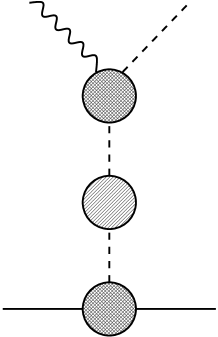
FIG. 2.: Pion pole term contributing to charged pion electroproduction.

FIG. 3.: Renormalized pion propagator. $Z$ is the wave function renormalization constant.

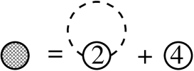
FIG. 4.: One-particle-irreducible pion self energy at ${\cal O}(p^{4})$. The vertices are derived from ${\cal L}_{2}$ and ${\cal L}_{4}$, denoted by 2 and 4 in the interaction blobs, respectively.

FIG. 5.: One-particle-irreducible electromagnetic vertex at ${\cal O}(p^{4})$ obtained from the “minimal Lagrangian.” The vertices are derived from ${\cal L}_{2}$ denoted by 2 in the interaction blobs.

FIG. 6.: Generic tree-level contribution at ${\cal O}(p^{4})$.

REFERENCES

- [1] A. Liesenfeld et al. [A1 Collaboration], Phys. Lett. B 468, 19 (1999).
- [2] J. Volmer et al. [The Jefferson Lab F(pi) Collaboration], Phys. Rev. Lett. 86, 1713 (2001).
- [3] A. M. Bincer, Phys. Rev. 118, 855 (1960).
- [4] H. W. Naus and J. H. Koch, Phys. Rev. C 36, 2459 (1987).
- [5] P. C. Tiemeijer and J. A. Tjon, Phys. Rev. C 42, 599 (1990).
- [6] N. M. Kroll and M. A. Ruderman, Phys. Rev. 93, 233 (1954).
- [7] M. Gell-Mann and M. L. Goldberger, Phys. Rev. 96, 1433 (1954).
- [8] E. T. Dressler, Can. J. Phys. 66, 279 (1988).
- [9] S. Nozawa and T. S. Lee, Nucl. Phys. A513, 511 (1990).
- [10] O. Hanstein, D. Drechsel, and L. Tiator, Nucl. Phys. A632, 561 (1998).
- [11] M. Guidal, J. M. Laget, and M. Vanderhaeghen, Nucl. Phys. A627, 645 (1997).
- [12] M. Vanderhaeghen, M. Guidal, and J. M. Laget, Phys. Rev. C 57, 1454 (1998).
- [13] H. Haberzettl, C. Bennhold, T. Mart, and T. Feuster, Phys. Rev. C 58, 40 (1998).
- [14] R. M. Davidson and R. Workman, Phys. Rev. C 63, 025210 (2001).
- [15] S. Scherer and H. W. Fearing, Phys. Rev. C 51, 359 (1995).
- [16] R. M. Davidson and G. I. Poulis, Phys. Rev. D 54, 2228 (1996).
- [17] H. W. Fearing, Phys. Rev. Lett. 81, 758 (1998).
- [18] H. W. Fearing and S. Scherer, Phys. Rev. C 62, 034003 (2000).
- [19] L. Heller, in The two-body force in nuclei, edited by S. Austin and G. Crawley (Plenum Press, New York, 1972).
- [20] K. Ohta, Phys. Rev. C 40, 1335 (1989).
- [21] J. W. Bos, S. Scherer, and J. H. Koch, Nucl. Phys. A 547, 488 (1992).
- [22] E. Kazes, Nuovo Cimento XIII, 1226 (1959).
- [23] G. Barton, Introduction to Dispersion Techniques in Field Theory (Benjamin, New York, 1965) Chap. 7.
- [24] F. A. Berends and G. B. West, Phys. Rev. 188, 2538 (1969).
- [25] J. C. Ward, Phys. Rev. 78, 182 (1950).
- [26] Y. Takahashi, Nuovo Cim. 6, 371 (1957).
- [27] H. W. L. Naus, Ph.D. thesis, Universiteit van Amsterdam, Amsterdam, 1990.
- [28] S. Pollock, H. W. Naus, and J. H. Koch, Phys. Rev. C 53, 2304 (1996).
- [29] H. W. Naus and J. H. Koch, Phys. Rev. C 39, 1907 (1989).
- [30] A. I. Lvov, Int. J. Mod. Phys. A 8, 5267 (1993).
- [31] S. Scherer, A. Yu. Korchin, and J. H. Koch, Phys. Rev. C 54, 904 (1996).
- [32] S. Kondratyuk and O. Scholten, nucl-th/9906044.
- [33] K. J. Barnes, Phys. Lett. 1, 166 (1962).
- [34] A. E. Kaloshin, Phys. Atom. Nucl. 62, 1899 (1999) [Yad. Fiz. 62, 2049 (1999)].
- [35] S. I. Nagorny and A. E. Dieperink, Eur. Phys. J. A 5, 417 (1999).
- [36] H. W. Fearing and S. Scherer, Few Body Syst. 23, 111 (1998).
- [37] T. E. Rudy, H. W. Fearing, and S. Scherer, Phys. Rev. C 50, 447 (1994).
- [38] R. L. Workman, H. W. Naus, and S. J. Pollock, Phys. Rev. C 45, 2511 (1992).
- [39] S. Scherer and H. W. Fearing, Nucl. Phys. A684, 499 (2001).
- [40] J. Gasser and H. Leutwyler, Annals Phys. 158, 142 (1984).
- [41] H. Leutwyler, BUTP-91-26, Lectures given at 30th Int. Universitätswochen für Kernphysik, Schladming, Austria, Feb 27 - Mar 8, 1991 and at Advanced Theoretical Study Inst. in Elementary Particle Physics, Boulder, CO, Jun 2-28, 1991.
- [42] S. Weinberg, Physica A 96, 327 (1979).
- [43] S. Kamefuchi, L. O’Raifeartaigh, and A. Salam, Nucl. Phys. 28, 529 (1961).
- [44] C. Unkmeir, S. Scherer, A. I. L’vov, and D. Drechsel, Phys. Rev. D 61, 034002 (2000).
- [45] D. Drechsel, G. Knöchlein, A. Metz, and S. Scherer, Phys. Rev. C 55, 424 (1997).
- [46] J. Gasser, M. E. Sainio and A. Svarc, Nucl. Phys. B307, 779 (1988).
- [47] M. Mojzis, Eur. Phys. J. C 2, 181 (1998).
- [48] N. Fettes, U. Meißner and S. Steininger, Nucl. Phys. A640, 199 (1998).
- [49] T. Becher and H. Leutwyler, JHEP 0106, 017 (2001).
- [50] S. Weinberg, Nucl. Phys. B363, 3 (1991).
- [51] C. Ordonez, L. Ray and U. van Kolck, Phys. Rev. C 53, 2086 (1996).
- [52] N. Kaiser, R. Brockmann and W. Weise, Nucl. Phys. A625, 758 (1997)
- [53] E. Epelbaum, W. Glöckle and U. Meißner, Nucl. Phys. A671, 295 (2000).