Two-Pion Exchange in proton-proton Scattering

W. R. Gibbs^a and Benoît Loiseau^b

^a New Mexico State University, Department of Physics,
^b LPNHE Université P. & M. Curie

(Received: )

We present calculations of the two-pion-exchange contribution to proton-proton scattering at 90^∘ using form factors appropriate for representing the distribution of the constituent partons of the nucleon. Talk given at MENU2001, George Washington University July 26-31, 2001

1 Introduction

The cross section and the spin-correlation observable, C_NN, measured in the region from 0 to 12 GeV/c P_lab at 90^o provide an excellent testing ground for our theories of hadronic interactions. These data have been the focus of a number of experimental[1] and theoretical studies[2]. There is an apparent simplification of the amplitude in the region from 4 GeV/c to 8 GeV/c. At 90 ^∘ the spin-correlation observable $C_{NN}$ has a constant value of about 0.07 which might indicate the dominance of a single mechanism. The simple quark exchange mechanism gives 1/3 for $C_{NN}$.

One pion exchange provides an important contribution below about 2 GeV/c. The exchange of two pions has been used as a basis for the NN interaction at low energies and it is reasonable to assume that it remains important at higher energies. We have calculated the box and crossed two-pion exchange Feynman graphs with nucleons as intermediate states. Even if this mechanism dominates one can not expect good quantitative agreement with the data due to the strong inelasticity of the NN interaction at these energies since distortion effects need to be considered. None the less, several questions can be raised and answered.

2 Two-pion Exchange Calculation

The full cross section is given by

$$\frac{d\sigma}{d\Omega}=\left(\frac{m^{2}}{4\pi E}\right)^{2}|M|^{2}.$$

where, for pseudo-scalar coupling and box kinematics M is

$$M_{PS}=g^{4}\frac{1}{(2\pi)^{4}}\int\frac{dq\left[\bar{u}(k^{\prime})\gamma_{5}(/{\!\!\!p}+m)\gamma_{5}u(k)\right]_{1}\left[\bar{u}(-k^{\prime})\gamma_{5}(/{\!\!\!p^{\prime}}+m)\gamma_{5}u(-k)\right]_{2}}{(p^{2}-m^{2}+i\epsilon)({p^{\prime}}^{2}-m^{2}+i\epsilon)(q^{2}-{\mu}^{2}+i\epsilon)({q^{\prime}}^{2}-{\mu}^{2}+i\epsilon)}.$$

In this expression the minus sign on $k$ and $k^{\prime}$ applies only to spatial components. Corresponding to the propagator for proton 1, we have

$$\bar{u}(k^{\prime})\gamma_{5}(/{\!\!\!p}+m)\gamma_{5}u(k)=\bar{u}(k^{\prime})\gamma_{5}[(p_{0}-E_{p})\gamma_{0}+E_{p}\gamma_{0}-\mbox{\boldmath$\gamma$}\cdot{\bf p}+m]\gamma_{5}u(k)$$

$$=-\bar{u}(k^{\prime})(p_{0}-E_{p})\gamma_{0}u(k)+2m\bar{u}(k^{\prime})\gamma_{5}\sum_{r}u_{r}(p)\bar{u}_{r}(p)\gamma_{5}u(k)$$

where the spinors $u_{r}(p)$ are on shell with energy $E_{p}\equiv\sqrt{{\bf p}^{2}+m^{2}}.$

The integral can be written as an operator in spin space in the form

$$M_{PS}=g^{4}\frac{1}{(2\pi)^{4}}\int\frac{dq\Theta_{1}(p)\Theta_{2}(p^{\prime})}{(p^{2}-m^{2})({p^{\prime}}^{2}-m^{2})(q^{2}-\mu^{2})({q^{\prime}}^{2}-\mu^{2})},$$

$${\rm where}\ \ \Theta_{1}(p)=\frac{1}{2m}\left\{\left(E_{p}-p_{0}\right)\left(E+m+\frac{\mbox{\boldmath$\sigma_{1}$}\cdot{\bf k}^{\prime}\mbox{\boldmath$\sigma_{1}$}\cdot{\bf k}}{E+m}\right)+\right.$$

$$\left.\frac{\left[(E+m)\mbox{\boldmath$\sigma_{1}$}\cdot{\bf p}-(E_{p}+m)\mbox{\boldmath$\sigma_{1}$}\cdot{\bf k}^{\prime}\right]\left[(E_{p}+m)\mbox{\boldmath$\sigma_{1}$}\cdot{\bf k}-(E+m)\mbox{\boldmath$\sigma_{1}$}\cdot{\bf p}\right]}{(E_{p}+m)(E+m)}\right\}.$$

In the case of pseudo-vector coupling the interaction is given by $\frac{f}{\mu}\bar{\psi}\gamma_{\mu}\gamma_{5}\mbox{\boldmath$\tau$}\cdot\partial^{\mu}\mbox{\boldmath$\phi$}_{\pi}\psi$ and the operator corresponding to the first proton propagator is

$$(p^{2}-m^{2})P_{PV}=-\frac{f^{2}}{\mu^{2}}\bar{u}(k^{\prime})/{\!\!\!q}^{\prime}\gamma_{5}(/{\!\!\!p}+m)/{\!\!\!q}\gamma_{5}u(k)$$

$$=\frac{f^{2}}{\mu^{2}}\bar{u}(k^{\prime})\gamma_{5}(p^{2}-m^{2})(/{\!\!\!p}+3m)\gamma_{5}u(k)+\frac{f^{2}4m^{2}}{\mu^{2}}\bar{u}(k^{\prime})\gamma_{5}(/{\!\!\!p}+m)\gamma_{5}u(k).$$

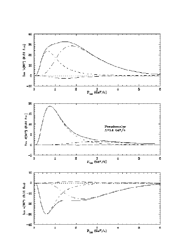
Figure 1: Contributions to the imaginary part of the b, d and e pseudo-scalar amplitudes. The short dash-dot line shows the result of placing the two nucleons on shell. The dashed and long dash-dot curves show the principal value parts from the box and cross diagrams respectively. The two-nucleons-on-shell contribution dominates at low energy but dies out at high energy where the amplitudes are dominated by the principal-value part of the crossed diagram.

The operator naturally separates into a term which corresponds to a contact term and one which is identical to the pseudo-scalar expression given before

$$P_{PV}=\frac{f^{2}}{\mu^{2}}\bar{u}(k^{\prime})\gamma_{5}(/{\!\!\!p}+3m)\gamma_{5}u(k)+g^{2}\frac{\bar{u}(k^{\prime})\gamma_{5}(/{\!\!\!p}+m)\gamma_{5}u(k)}{p^{2}-m^{2}}=P_{C}+P_{PS}.$$

Defining an operator analogous to $\Theta_{1}(p)$ for the contact term for the first proton

$$C_{1}(p)=\frac{E+m}{2m}\left[E_{p}-p_{0}+2m+\left(E_{p}-p_{0}-2m\right)\frac{\mbox{\boldmath$\sigma_{1}$}\cdot{\bf k}^{\prime}\mbox{\boldmath$\sigma_{1}$}\cdot{\bf k}}{(E+m)^{2}}\right]+$$

$$\frac{\left[(E+m)\mbox{\boldmath$\sigma_{1}$}\cdot{\bf p}-(E_{p}+m)\mbox{\boldmath$\sigma_{1}$}\cdot{\bf k}^{\prime}\right]\left[(E_{p}+m)\mbox{\boldmath$\sigma_{1}$}\cdot{\bf k}-(E+m)\mbox{\boldmath$\sigma_{1}$}\cdot{\bf p}\right]}{2m(E_{p}+m)(E+m)},$$

we can write

$$M_{PV}=\frac{g^{4}}{16m^{4}}\frac{1}{(2\pi)^{4}}\int dq\frac{C_{1}(p)C_{2}(p^{\prime})}{(q_{0}^{2}-\omega^{2})(q_{0}^{2}-{\omega^{\prime}}^{2})}+\frac{g^{4}}{4m^{2}}\frac{1}{(2\pi)^{4}}\int dq\frac{C_{1}(p)\Theta_{2}(p^{\prime})}{({p^{\prime}}^{2}-m^{2})(q_{0}^{2}-\omega^{2})(q_{0}^{2}-{\omega^{\prime}}^{2})}$$

$$+\frac{g^{4}}{4m^{2}}\frac{1}{(2\pi)^{4}}\int dq\frac{\Theta_{1}(p)C_{2}(p^{\prime})}{(p^{2}-m^{2})(q_{0}^{2}-\omega^{2})(q_{0}^{2}-{\omega^{\prime}}^{2})}+M_{PS}.$$

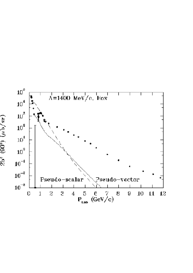
Figure 2: The calculation of $2|b|^{2}$ for the box diagram. The dashed line shows the result for the pseudo-scalar coupling and the solid line that of the pseudo-vector.

3 Proton Structure

The expressions in the previous section lack the form factors which are associated with each pion-nucleon vertex. We treat the two protons as particles with intrinsic size related to the distribution of (primarily) constituent quarks in the nucleon, assuming that the underlying interaction of the pions is with the partons. The form factor can be directly obtained as the Fourier transform of the density[3]. Such a derivation is inherently non-relativistic since it is not expressed in terms of Lorentz invariants.

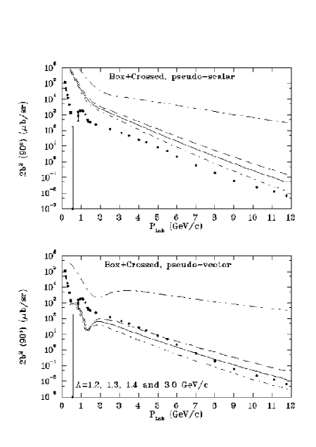
Figure 3: Dependence of $|b|^{2}$ on the value of $\Lambda$. The smaller values of the partial cross sections correspond to the smaller values of $\Lambda$ in order.

An exponential parton density leads to the form, $(\alpha^{2}-\mu^{2})^{2}/({\bf q}^{2}+\alpha^{2})^{2}$. A common relativistic generalization is

$$\frac{(\alpha^{2}-\mu^{2})^{2}}{(q_{0}^{2}-{\bf q}^{2}-\alpha^{2})^{2}},$$

but this procedure introduces an additional singularity in $q_{0}$ on the real axis.

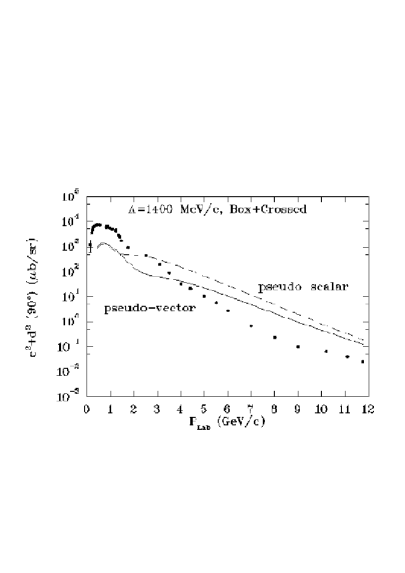
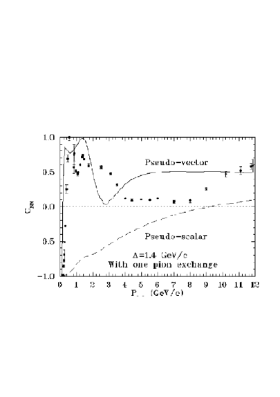
Figure 4: Left: Dependence of $|e|^{2}+|d|^{2}$ on the type of coupling. Right: Comparison with the experimental values of $C_{NN}$ for the different couplings.

A second generalization of ${\bf q}^{2}$ can be obtained by the following argument. The form factor must be a function of Lorentz scalars only. There are three four-vectors, the initial and final nucleon momenta (k,k’) and the pion momentum (q) of which only two are independent. Choose one of the nucleon momenta (k) and the pion momentum (q). From these we can construct three scalars $q^{2},\ k^{2},\ \ {\rm and}\ \ k\cdot q.$ In order to be homogeneous in k and q, the only two invariants we can consider are $(k\cdot q)^{2}$ and $k^{2}q^{2}$. The linear combination $(k\cdot q)^{2}-k^{2}q^{2}$ reduces to $m^{2}{\bf q}^{2}$ if the nucleon is on shell at rest. We use the generalization

$${\bf q}^{2}\rightarrow Q^{2}(k,q)\equiv\frac{(k\cdot q)^{2}-k^{2}q^{2}}{m^{2}},$$

which has the property $Q^{2}(k\pm q,q)=Q^{2}(k,q)$. Either the initial or final nucleon momentum may be used. A number of authors have used a similar form in one way or another[4].

One can also be led to this expression by the requirement that $Q^{2}(k,q)=Q^{2}(k^{\prime},q)$. Since $k^{\prime}=k+q$ (for example) this condition is suggestive of the vector cross product. The four-dimensional cross product is defined by the use of a totally antisymmetric 4-component tensor, $\epsilon_{ijk\ell}$. Since we still have only two vectors (say a and b) the result is a tensor

$$T_{ij}=\sum_{k,\ell=0,1,2,3}\epsilon_{ijk\ell}a_{k}b_{\ell},$$

with 6 independent components. We can separate the components into two classes: one in which the zero index is free and one in which it is summed over

$$T_{0j}=\sum_{k,\ell=1,2,3}\epsilon_{0jk\ell}a_{k}b_{\ell}=[{\bf a}\times{\bf b}]_{j},$$

$$T_{ij}=a_{0}b_{k}-b_{0}a_{k}=[a_{0}{\bf b}-b_{0}{\bf a}]_{k},\ \ \ i,j,k\ \ {\rm cyclic}\neq 0.$$

Contracting this tensor with the metric tensor we find

$$\frac{1}{2}\sum g_{ii^{\prime}}g_{jj^{\prime}}T_{ij}T_{i^{\prime}j^{\prime}}=\frac{1}{2}\sum g_{ii}g_{jj}T_{ij}T_{ij}=(a_{0}{\bf b}-b_{0}{\bf a})^{2}-({\bf a}\times{\bf b})^{2}\equiv(a\cdot b)^{2}-a^{2}b^{2}.$$

In general, two invariants are available, $(k\cdot q)^{2}/m^{2},$ which evaluates to $q_{0}^{2}$ in the rest frame of the nucleon and $[(k\cdot q)^{2}-k^{2}q^{2}]/m^{2}$, which evaluates to $|{\bf q}|^{2}$. We could choose any combination of $|{\bf q}|^{2}$ and $q_{0}^{2}$ for the variable in the rest frame. Only $[(k\cdot q)^{2}-k^{2}q^{2}]/m^{2}$ and $q^{2}$ are independent of which nucleon momentum ($k$ or $k^{\prime}$) is used.

By choosing a function independent of $q_{0}$ in the nucleon rest frame, the interaction is instantaneous, perhaps a physically reasonable choice since the valence quarks are always present, hence they do not have a formation time. For the present calculation we can always choose the nucleon to be one of the external lines, and hence on shell. We use

$$f(k,q)=f({\bf k},q_{0},{\bf q})=\left[\frac{\Lambda^{2}}{(k\cdot q/m)^{2}-q^{2}+\Lambda^{2}}\right]^{2}.$$

A product of four of these factors will appear, one for each vertex. For the box diagram we have

$$f({\bf k},q_{0},{\bf q})f(-{\bf k},q_{0},{\bf q})f({\bf k}^{\prime},q_{0},{\bf q}^{\prime})f(-{\bf k}^{\prime},q_{0},{\bf q}^{\prime}),$$

while for the crossed diagram the factors are

$$f({\bf k},q_{0},{\bf q}^{\prime})f(-{\bf k},q_{0},{\bf q})f({\bf k}^{\prime},q_{0},{\bf q})f(-{\bf k}^{\prime},q_{0},{\bf q}^{\prime}).$$

The difference in the variables appearing in these expressions has important consequences for the behavior of the box and crossed graphs.

The off-shell range in the calculation, $\Lambda$, which corresponds to the extension of the proton distribution of partons can be evaluated from other sources. Coon and Scadron[5] found $\Lambda$ between 0.8 and 1.0 GeV/c for a monopole form. To convert to an equivalent dipole form at low momentum transfer one can multiply by $\sqrt{2}$ giving a range from 1.13 to 1.41 GeV/c. In lattice QCD calculations Liu, Dong and Draper[6] find $\Lambda$ =0.747 GeV/c for a monopole form and $\Lambda$=1.32 GeV/c for a dipole.

We use a dipole form and most of the calculations shown will be for $\Lambda$=1.4 GeV/c.

4 Results

To describe nucleon-nucleon scattering we use the amplitudes defined by the Saclay group[7] given by the equation

$$M({\bf k}_{f},{\bf k}_{i})=\frac{1}{2}[(a+b)+(a-b)\mbox{\boldmath$\sigma_{1}$}\cdot{\bf n}\mbox{\boldmath$\sigma_{2}$}\cdot{\bf n}+(c+d)\mbox{\boldmath$\sigma_{1}$}\cdot{\bf m}\mbox{\boldmath$\sigma_{2}$}\cdot{\bf m}+(c-d)\mbox{\boldmath$\sigma_{1}$}\cdot{\bf l}\mbox{\boldmath$\sigma_{2}$}\cdot{\bf l}+e(\mbox{\boldmath$\sigma_{1}$}+\mbox{\boldmath$\sigma_{2}$})\cdot{\bf n}]$$

with ${\bf l}=\frac{{\bf k}_{f}+{\bf k}_{i}}{|{\bf k}_{f}+{\bf k}_{i}|},\ {\bf m}=\frac{{\bf k}_{f}-{\bf k}_{i}}{|{\bf k}_{f}-{\bf k}_{i}|},\ {\bf n}=\frac{{\bf k}_{i}\times{\bf k}_{f}}{|{\bf k}_{i}\times{\bf k}_{f}|}\ .$

With identical particle symmetry $a(90^{\circ})=0$ and $c(90^{\circ})=-b(90^{\circ})$, so only 3 amplitudes are needed to describe the scattering. At $90^{\circ}$

$$\sigma=\frac{1}{2}(2|b|^{2}+|d|^{2}+|e|^{2});\ \ \sigma C_{NN}=\frac{1}{2}(-2|b|^{2}+|d|^{2}+|e|^{2}),$$

so from the data we can extract $2|b|^{2}$ and $|d|^{2}+|e|^{2}$ directly.

Figure 1 shows the amplitudes coming from different types of contribution for pseudo-scalar coupling. The case of pseudo-vector coupling is similar. We see that the important contributors are different at high and low energies. Figure 2 shows the results of the box diagram for PS and PV coupling for the partial cross section $|b|^{2}$. While the contribution of this diagram falls rapidly, the crossed diagram falls much more slowly as one can see from Figure 3 which shows the sum for various values of $\Lambda$. Clearly the crossed diagram dominates at high energy. This difference can be traced to the difference in the variables in the form factors as mentioned above. We also see a very large sensitivity to the value of the off-shell range which is very natural since the fall-off of the cross section is given primarily by the form factor.

Figure 4 (left) shows the result of the sum of the box and crossed diagrams for the sum $d^{2}+e^{2}$.

We see that each case there is a large difference between PS and PV coupling, as pointed out (at lower energies) by Robilotta et al.[8]. However, the PS and PV couplings can be mixed. Gross et al.[9] found 1/4 PS and 3/4 PV. Goudsmit et al.[10] found a small mixture of PS (about 3%).

Kondratyuk and Scholten[11] found a mixture which varied with momentum transfer, being dominated by PV at low values and about equal at higher values. This is expected since chiral symmetry imposes pseudo-vector coupling a low energy.

Figure 4 (right) shows a comparison with the spin correlation observable. We see that the PS and PV results bracket the data.

The underlying structure of the proton, represented here by the form factor, plays an essential role in the scattering in this energy range.

Our conclusions are: 1) two pion exchange gives a significant contribution to pp scattering in this energy region, 2) the crossed graph dominates over the box at high energies 3) the important contributions at high energies are different than at low energies and 4) there is a significant reduction of the cross section for PV coupling compared to PS coupling similar to that seen in low-energy pion-nucleon scattering.

Acknowledgments:  The LPNHE is a Unité de Recherche des Universités Paris 6 et Paris 7, associée au CNRS. This work was supported by the U. S. Department of Energy and the National Science Foundation.

References

• [1] G. R. Court et al., Phys. Rev. Lett. 57, 507 (1986); T. S. Bhatia et al., Phys. Rev. Lett. 49, 1135 (1982); E. A. Crosbie et al., Phys. Rev. D23, 600 (1981); A. Lin et al., Phys. Rev. Lett. 41, 1257 (1978); D. G. Crabb et al, Phys. Rev. Lett. 41, 1257 (1978); J. R. O’Fallon et al., Phys. Rev. Lett. 39, 733 (1977).
• [2] S. J. Brodsky, C. E. Carlson and H. Lipkin, Phys. Rev. D20, 2278 (1979); Glennys R. Farrar, Steven Gottlieb, Dennis Sivers and Gerald H. Thomas, Phys. Rev. D20, 202 (1979); Gordon P. Ramsey and Dennis Sivers, Phys. Rev. D45, 79 (1992), Phys. Rev. D47, 79 (1993).
• [3] W. R. Gibbs and B. Loiseau, Phys. Rev. C50, 2742 (1994).
• [4] G. Ramalho, A. Arriaga and M. T. Peña, Phys. Rev. C60, 047001 (1999); B. D. Keister and L. S. Kisslinger, Nucl. Phys. A326, 445 (1979); G. Wolf, Phys. Rev. 182, 1538 (1969); H. P. Durr and H. P. Pilkuhn, Nuovo Cim. 40, 899 (1965); J. Benecke and H. P. Durr, Nuovo Cim. 56, 269 (1968).
• [5] S. A. Coon and M. D. Scadron, Phys. Rev. C42, 2256 (1990); Phys. Rev. C23, 1150 (1981).
• [6] K. F. Liu, S. J. Dong and T. Draper, Phys. Rev. Lett. 74, 2172 (1995).
• [7] J. Bystricky, F. Lehar, and P. Winternitz, J. Phys. 39, 1 (1978).
• [8] M. R. Robilotta and C. A. da Rocha, Nucl. Phys. A615, 391 (1997).
• [9] F. Gross and Y. Surya, Phys. Rev. C47, 73 (1993).
• [10] P. F. A. Goudsmit, H. J. Leisi, E. Matsinos, B. L. Birbrair and A. B. Gridnev, Nucl. Phys. A575, 673 (1994).
• [11] S. Kondratyuk and O. Scholten, Phys. Rev. C59, 1070 (1999).