Hydrodynamical analysis of flow at RHIC

Abstract

We use a hydrodynamical model to describe the evolution of the collision system at collision energies $\sqrt{s}=130$ and 200 GeV. At lower $\sqrt{s}=130$ GeV energy we compare the results obtained assuming fast or slow thermalization (thermalization times $\tau_{0}=0.6$ and 4.1 fm/$c$, respectively) and show that slow thermalization fails to reproduce the observed anisotropy of particle distribution. At $\sqrt{s}=200$ GeV collision energy our results show anisotropies similar to those observed at $\sqrt{s}=130$ GeV.

1 Introduction

The azimuthal anisotropy of particle distributions in heavy ion collisions is a signal of rescattering among the particles. The larger the anisotropy, the stronger the rescattering. Since the hydrodynamical models assume zero mean free path and thus infinite scattering rate, they provide an upper limit to observable anisotropies. In our earlier papers Kolb:2001 ; Huovinen:2001 ; Kolb:2001b we have argued that since the observed anisotropies are well reproduced by a hydrodynamical model, the collision system must thermalize fast. Here we constrain our model further by requiring it to reproduce the observed single particle $p_{t}$-distributions Velkovska:2001 and study the consequences of such a long thermalization time that there is no thermal plasma but the hydrodynamical expansion begins in hadronic phase. We also tune our model to reproduce the charged particle multiplicity at $\sqrt{s}=200$ GeV collision energy published recently by the PHOBOS collaboration Phobos and show our results for the charged particle anisotropy and pion and antiproton $p_{t}$-spectra at the higher energy.

2 Hydrodynamical model and its initialization

To reduce the complexity of the numerical calculations we assume boost invariant scaling flow in our hydrodynamical model and solve the equations numerically only in the two transverse dimensions. We also apply ideal fluid hydrodynamics and assume that viscous effects are negligible. Depending on the initialization we apply two different equations of state: one with a phase transition at $T_{c}=165$ MeV or purely hadronic equation of state, called EoS A and H in Kolb:2001 , respectively.

In our model we assume that the chemical and kinetic freeze-out take place at the same temperature. In other words the system maintains both kinetic and chemical local equilibrium during the entire evolution from thermalization to freeze-out. This makes it impossible for us to fit both proton and antiproton yields simultaneously since the thermal model studies Xu:2001 point to chemical freeze-out temperatures much higher than the kinetic freeze-out temperature $T_{f}=100$ – 140 MeV required to produce sufficiently flat $p_{t}$-spectra. We counter this problem by the following approximation: We fix our initial baryon density to reproduce the observed $\bar{p}/p\sim 0.6$ Back:2001 ratio at $T=165$ MeV, i.e. immediately after the system has hadronized. We then let the system evolve to its freeze-out temperature and scale the calculated proton and antiproton yields to their values at $T=165$ MeV by hand. This scaling factor depends on the kinetic freeze-out temperature and has to be adjusted accordingly.

2.1 Fast thermalization

We have discussed different ways to parametrize the initial state of hydrodynamic evolution in Kolb:2001b . It was found that neither a parametrization where the density (energy or entropy) is proportional to the local number of participants or binary collisions is sufficient to reproduce the observed centrality dependence of multiplicity Adcox:2001 . A combination of these like the two component model presented in Kharzeev:2001 is required instead.

To obtain the results presented here we have used a combination of parametrizations eWN and eBC described in Kolb:2001b . In this case we assume the initial energy density to be proportional to the scaled sum of number of participants and binary collisions per unit area:

$$e(\mathbf{s},\tau_{0};\mathbf{b})=xK_{e}(\tau_{0})n_{\mathrm{WN}}(\mathbf{s;b})+(1-x)\tilde{K}_{e}(\tau_{0})n_{\mathrm{BC}}(\mathbf{s;b}),$$ (1)

where $n_{\mathrm{WN}}(\mathbf{s;b})$ is the number of participants and $n_{\mathrm{BC}}(\mathbf{s;b})$ the number of binary collisions per unit area in the transverse plane. The normalization constants $K_{e}(\tau_{0})$ and $\tilde{K}_{e}(\tau_{0})$ are the same than in Kolb:2001b and the mixing parameter $x=0.4$ was found to reproduce the observed centrality dependence of multiplicity. The equation of state with phase transition (EoS A) has been used to calculate results with short thermalization time ($\tau_{0}=0.6$ fm).

2.2 Slow thermalization and free streaming

The parametrization described above is reasonable if thermalization time is sufficiently small and produced particles do not have time to move far away from the place where they were produced. On the other hand, if it takes several fermi for the system to thermalize, the particles will move during thermalization and smear any structure in the system.

To estimate what the shape and distributions of the system might be after a long thermalization process, we developed further the ideas outlined in Kolb:2000 . We approximate the expansion of the system during thermalization by free streaming. In this approach the number density of initially produced excitations is again taken to be proportional to the scaled sum of number of participants and binary collisions whereas the momentum distribution is taken to be that of pions at temperature of $T=200$ MeV. The free streaming is allowed to continue until thermalization time $\tau_{0}$ when energy density distribution due to free streaming particles is calculated and taken to be the thermal energy distribution. In this approximation we do not assign any radial velocity to the system at the end of free streaming. The effects of build-up of flow during thermalization will be discussed in KTHH .

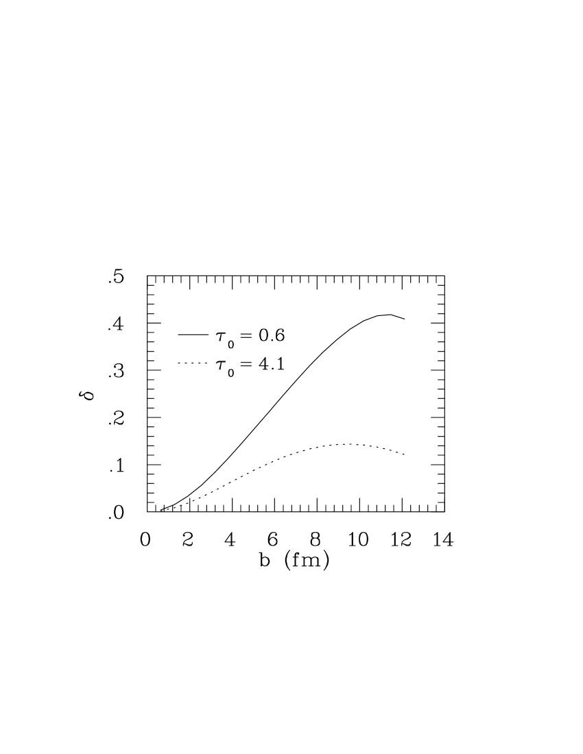
Figure 1: Initial energy density distribution in $b=2.4$ fm collision scaled by maximum energy density (left) and initial spatial deformation of the system as function of impart parameter (right) using parametrizations for fast and slow thermalization.

The distribution of particles in a free streaming system is given by Heiselberg:1999

$$n(\mathbf{x,p},\tau_{0})=f_{0}(p_{t},p^{\prime}_{z})\,S_{\perp}(\mathbf{s-v}_{\perp}(\tau_{0}-\tau_{i}),\mathbf{b}),$$ (2)

where $S_{\perp}(\mathbf{s,b})\propto xK_{n}n_{\mathrm{WN}}(\mathbf{s;b})+(1-x)K_{b}n_{\mathrm{BC}}(\mathbf{s;b})$ gives the density distribution of the initial excitations and $f_{0}(p_{t},p_{z})$ is Boltzmann distribution. Of the parameters $p^{\prime}_{z}=\tau_{0}p_{z}/\tau_{i}$ is the scaled longitudinal momentum which takes longitudinal free streaming in boost invariant system into account, $\tau_{0}$ is thermalization time and $\tau_{i}$ is the time when the distributions before free streaming are specified. We use $\tau_{i}=0.6$ fm and fix thermalization time by requiring that maximum temperature in central collisions is low enough for hadrons to exist. We choose this somewhat arbitrary limit to be $T=200$ MeV. This corresponds to $\epsilon=2.3$ GeV/fm³ in the hadronic equation of state (EoS H) we use with this initial state. After the remaining parameters $K_{n}$, $K_{b}$ and $x$ are chosen to reproduce the observed centrality dependence of multiplicity Adcox:2001 , this procedure leads to a thermalization time $\tau_{0}=4.1$ fm.

As shown in Fig. 1 this parametrization leads to a larger system which density gradients are flatter and the spatial deformation smaller than in the fast thermalization parametrization (Eq.(1)).

3 Comparison to observables

3.1 $p_{t}$-distributions

After fixing the proportionality constants $K_{e}$ and $\tilde{K}_{e}$ and mixing $x$ in Eq.(1) the only remaining parameter in our model is the freeze-out temperature. We fix it to reproduce the preliminary $p_{t}$-distributions of pions and antiprotons in most central collisions measured by the PHENIX Collaboration Velkovska:2001 . This requirement leads to very different temperatures. If early thermalization is assumed, $T_{f}\approx 140$ MeV leads to a nice fit. On the other hand long thermalization time and free streaming of particles during thermalization smoothens the pressure gradients so much that a low freeze-out temperature of $T_{f}\approx 100$ MeV is needed to create large enough transverse flow (Fig.(2)). This difference in freeze-out temperatures leads also to very different scaling factors for the antiproton yield, 2 and 27 for $\tau_{0}=0.6$ fm and $\tau_{0}=4.1$ fm, respectively. After scaling the yields to their values at $T_{ch}=165$ MeV, we reach an acceptable reproduction of measured spectra in most central collisions.

Having the parameters of our models fixed we can now compare our results to spectra of non-central collisions Velkovska:2001 (see Fig. 2). The average number of participants in five different centrality classes Burward-Hoy set our choice of impact parameter in these bins to 2.4, 5.1, 7.0, 9.6 and 12.1 fm, respectively. The early thermalization assumption leads to very good agreement with the preliminary data even for the most peripheral collisions. On the other hand, the late thermalization approach performs adequately in central and semi-central collisions, but leads to far too steep slopes in peripheral collisions. This failure could be expected since if one assumes a long thermalization time even in central collisions, it is probable that the system does not thermalize at all in peripheral collisions and our model fails.

Figure 2: $p_{t}$ distributions of negative pions (left) and antiprotons (right) at $\sqrt{s}=130$ collision energy compared with preliminary PHENIX data Velkovska:2001 . The data and curves correspond to centralities $\sigma/\sigma_{\mathrm{tot}}=0$-5%, 5-15%, 15-30%, 30-60%, 60-92% and impact parameters $b=2.4$, 5.1, 7.0, 9.6 and 12.1 fm, respectively (top to bottom). These data sets are successively scaled down by $10^{-n}$,$n=0$,1,2,3,4.

3.2 Azimuthal anisotropy

So far we have used different observables to fix parameters of our model and the real test is in the comparison to the observed anisotropies of particle distribution Adler:2001 ; Snellings:2001 . As we have reported in our earlier papers Kolb:2001 ; Huovinen:2001 ; Kolb:2001b , hydrodynamical model leads to an excellent fit to observed data if thermalization time is short. We show our present results in Fig.(3). The present parametrization ($\tau_{0}=0.6$ fm) leads to a slightly smaller differential anisotropy for pions and larger anisotropy for antiprotons than shown in our previous works. Both changes are mainly due to higher freeze-out temperature (see Huovinen:2001 ). The deviation from data is still within systematical error and as reported in this conference Tang , more careful analysis of the data to make systematic errors smaller may lead to slightly smaller $v_{2}$. Also we want to remind that our present fit to freeze-out temperature $T_{f}\approx 140$ MeV is preliminary and may change when we fit more data and explore different parameter combinations.

Figure 3: Differential anisotropy of pions and protons+antiprotons (upper and lower curve, respectively) in minimum bias collisions compared to preliminary data Adler:2001 .

On the other hand the results for long thermalization time approach are well below the data and show that – at least in the present formulation – the free streaming period changes the shape of the initial system sufficiently to prevent the build-up of observed anisotropies. This corroborates our earlier argument that early thermalization is necessary to achieve the observed large anisotropies in particle distributions.

4 Collisions at $\sqrt{s}=200$ GeV

Figure 4: $p_{t}$ distributions of pions and antiprotons at 5% most central $\sqrt{s}=130$ and 200 GeV collisions (left) and differential anisotropy of charged particles in minimum bias $\sqrt{s}=130$ and 200 GeV collisions compared with preliminary STAR data at $\sqrt{s}=130$ GeV Snellings:2001 (right).

We use the charged particle multiplicity $dN/d\eta=650\pm 35$ in 6% most central collisions measured recently by the PHOBOS Collaboration Phobos to fix our parametrization for $\sqrt{s}=200$ GeV collisions. We assume that all the other parameters like freeze-out temperature ($T_{f}\approx 140$ MeV) and thermalization time ($\tau_{0}=0.6$ fm) stay unchanged. We do not have any method to calculate the change in baryon stopping and thus the change in initial baryon density. Therefore we ignore the question of the change in stopping altogether and use the same initial baryon density at both energies. For the same reason we do not scale the calculated antiproton yield at freeze-out either but show the result as it is to demonstrate the change in slopes.

The calculated pion and antiproton distributions at $\sqrt{s}=130$ and 200 GeV are shown in Fig.(4). The changes in slopes are small but still large enough to increase $E_{t}$ by $\sim 18\%$ even if the observed increase in particle multiplicity is $14\%$ Phobos . Our calculation leads to the increase of the average energy density at $\tau=1$ fm from 5.4 to 6.8 GeV/fm³ and the increase of the maximum temperature (at $\tau_{0}=0.6$ fm) from 355 to 375 MeV. If the changes in $p_{t}$-spectra are small they are even tinier in anisotropies. In Fig.(4) differential anisotropy for charged particles in minimum bias collisions is shown with preliminary STAR data for $\sqrt{s}=130$ GeV collision. The change is negligible and it will be interesting to see whether the data deviates from the calculation around $p_{t}\approx 2$ GeV also at $\sqrt{s}=200$ GeV collision energy.

5 Summary

We have shown that it is possible to fit both the experimental $p_{t}$ spectra and anisotropy of particle distribution if short thermalization time and hydrodynamical behaviour of the collision system is assumed. On the other hand long thermalization time allows the system shape change too much before the build-up of flow begins and generates sufficient anisotropies. This corroborates our earlier argument that fast thermalization is required to explain the experimental data.

We have also made the first calculations at $\sqrt{s}=200$ GeV collision energy. Our results show only slightly flatter spectra and basically no change in differential $v_{2}$ when compared to results at lower $\sqrt{s}=130$ GeV energy.

References

- (1) P. F. Kolb, P. Huovinen, U. Heinz and H. Heiselberg, Phys. Lett. B 500, 232 (2001) [hep-ph/0012137].
- (2) P. Huovinen, P. F. Kolb, U. Heinz, P. V. Ruuskanen and S. A. Voloshin, Phys. Lett. B 503, 58 (2001) [hep-ph/0101136].
- (3) P. F. Kolb, U. Heinz, P. Huovinen, K. J. Eskola and K. Tuominen, hep-ph/0103234.
- (4) J. Velkovska [PHENIX collaboration], nucl-ex/0105012.
- (5) B. Wyslouch, these proceedings; B. B. Back et al. [PHOBOS Collaboration], nucl-ex/0108009.
- (6) N. Xu and M. Kaneta, nucl-ex/0104021; P. Braun-Munzinger, D. Magestro, K. Redlich and J. Stachel, hep-ph/0105229; W. Florkowski, W. Broniowski and M. Michalec, nucl-th/0106009.
- (7) B. B. Back et al. [PHOBOS Collaboration], hep-ex/0104032; C. Adler [the STAR Collaboration], Phys. Rev. Lett. 86, 4778 (2001) [nucl-ex/0104022]; I. G. Bearden et al. [BRAHMS Collaboration], nucl-ex/0106011.
- (8) K. Adcox et al. [PHENIX Collaboration], Phys. Rev. Lett. 86, 3500 (2001) [nucl-ex/0012008]; B. B. Back et al. [PHOBOS Collaboration], nucl-ex/0105011.
- (9) D. Kharzeev and M. Nardi, Phys. Lett. B 507, 121 (2001) [nucl-th/0012025].
- (10) P. F. Kolb, J. Sollfrank and U. Heinz, Phys. Rev. C 62, 054909 (2000) [hep-ph/0006129].
- (11) P. F. Kolb, M. Tilley, P. Huovinen, and U. Heinz in preparation.
- (12) H. Heiselberg and A. Levy, Phys. Rev. C 59, 2716 (1999) [nucl-th/9812034]; G. Baym, Phys. Lett. B 138, 18 (1984).
- (13) J. Burward-Hoy, private communication.
- (14) C. Adler et al. [STAR Collaboration], nucl-ex/0107003.
- (15) R. J. Snellings [STAR Collaboration], nucl-ex/0104006.
- (16) A.H. Tang, these proceedings.