Faddeev Approach to the Study of One- and Two-hole Spectral Functions

Abstract

Theoretical calculations of one- and two-hole spectral functions for the ${}^{16}{\rm O}$ nucleus are still failing to describe some of the important features observed experimentally. Of critical importance for the solution of these issues is to obtain an appropriate description of the interplay between hole-hole and particle-hole excitations. A formalism is reviewed here that allows the consistent treatment of such phonons at a Random Phase approximation level. Although the application of this formalism to ${}^{16}{\rm O}$ is still in the implementation stage, some preliminary results are discussed here.

I Introduction

As a result of correlations between nucleons inside the nuclear medium, the occupation probability of single-particle shells are lowered with respect to the mean-field prediction. Experimentally, this can be observed as a quenching of the absolute spectroscopic factors for the knockout of a nucleon from a given shell. Studies of $(e,e^{\prime}p)$ reactions have allowed the determination of spectroscopic factors in many closed-shell nuclei diep ; sick ; Lapik demonstrating that the removal probability for nucleons from these systems is reduced by about 35% with respect to the shell-model predictions.

For the ${}^{16}{\rm O}$ nucleus, the experimental spectroscopic strength leus for the knockout of a proton from both the $p_{1/2}$ and $p_{3/2}$ shells corresponds to about $60\%$. The inclusion of relativistic effects in the analysis of data is espected to change these results by not more than a few % udias . Theoretical calculations for this nucleus seem still far from being able to reproduce quantitatively the experiments and give numbers that depend on the approximation scheme employed. Variational calculations, focussed on short-range correlations, yield about a 10% of strength removal rad94 ; md94 ; Fabr01 before the effects of the center of mass motion are included. Center of mass corrections are known to raise the spectroscopic factor by about 7% O16jast , thus worsening the agreement with data. An improvement of these results seems to require a treatment of low-energy correlations with the inclusion two-hole–one-particle (2h1p) states FabrNM ; fabrconf . This would be in line with the Green’s function calculations of Ref. GeurtsO16 , in which 2h1p states were taken into account and a reduction of about 25% was obtained, still neglecting center of mass corrections. A comparison with the experimental result (and their uncertainties) suggests that about 20% of the observed single-particle strength removal remains unexplained. Nevertheless, it is important to note that the results of Ref. GeurtsO16 indicate the low-energy correlations as an essential ingredient, needed for a complete understanding of this puzzle.

The merit of the calculation of Ref. GeurtsO16 lies in the fact that summing 2h1p states and their interactions to all orders, one can achieve a simultaneous description of the effects of both particle-hole (ph) and hole-hole (hh) collective excitations, including the interplay between them. These effects, though, were accounted for only at a Tamm-Dancoff approximation (TDA) level. In order to account for the coupling to collective excitations that are actually observed in ${}^{16}{\rm O}$ it is necessary to at least consider a Random-Phase approximation (RPA) description of the isoscalar negative parity states czer . To account for the low-lying isoscalar positive parity states an even more complicated treatment will be required. Sizable collective effects are also present in the particle-particle (pp) and hh excitations involving tensor correlations for isoscalar and pair correlations for isovector states.

Taking a look at the experimental spectral function leus , one can also notice that the total strength for proton emission of a $p_{3/2}$ proton is experimentally distributed over a main peak and two small fragments at slightly higher missing energy. This splitting is not described by the calculations of Ref. GeurtsO16 where only one pole is generated that contains most of the single-particle strength.

The results of Ref. GeurtsO16 have been used as a starting point to study the ¹⁶O(e,e^′pp) reaction geurts2h ; geueepp . In these works, the two-hole spectral function was obtained by coupling two dressed single-particle (sp) propagators and then allowing them to interact to all orders through a ladder type equation. The distortaion of the two-hole overlap function caused by short-range effects was also included by adding defect functions associated with a G-matrix interaction CALGM which was computed for the finite ${}^{16}{\rm O}$ nucleus. These calculations led to a proper description of the experimental cross section for two proton emission ond1 ; ond2 and yield amplitudes for the transition to the ground state of ${}^{14}{\rm C}$ and to some of its lowest excited states.

Nevertheless a completely satisfactory description is missing here also. Recent developments of NN knockout reactions allow to distinguish several states of the final nucleus and in particular it is now possible to disentangle the two $2^{+}$ excited states of ${}^{14}{\rm C}$  at 7.0 and 8.32 MeV exp1 ; exp2 . In spite of this, the theoretical calculations of Ref. geurts2h can generate only one $2^{+}$ excited state. It is interesting to note that the transition to both of the $2^{+}$ states can be interpreted as the knockout of two protons from a $p_{1/2}$ and a $p_{3/2}$ state. Although this has not been directly investigated yet, it comes natural to suppose that the fragmentation of the $p_{3/2}$ peak seen in the ¹⁶O(e,e^′p) reaction could play some role in the generation of the $2^{+}$ doublet in ${}^{14}{\rm C}$. Moreover, it must be noted that the strength of the $p_{1/2}$ and $p_{3/2}$ peaks, generated in the calculations of the one-hole spectral function, enters directly in the calculation of the two-hole amplitude.

It is therefore evident that one- and two-hole spectral functions are closely related, the correct description of the first being relevant for a successful description of the second and vice versa. As a consequence, a formalism in which both quantities are generated together in a consistent way is highly desirable. This can be achieved in the the framework of self-consistent Green’s function theory (SCGF) in which the equations of motion are expressed in terms of fragmented propagators and are iterated until self-consistency is reached.

At the same time, it is also desirable to extend the calculations of Ref. GeurtsO16 to include the RPA description of pp (hh) and ph phonons. This is not completely trivial. For example, the naive summation of diagrams containing both pp and ph phonons leads to serious inconsistencies. This approximation is depicted in Fig. 1. The last of the three diagrams on the right hand side is already contained in each of the other two and must therefore be subtracted to avoid double counting. This subtraction introduces spurious poles in the Lehmann representation of the self-energy and generates meaningless (not even normalizable) solutions of the Dyson equation. In addition, each of the first two terms in Fig. 1 ignores the Pauli correlations between the freely propagating line and the quasi-particles forming the phonons, as noted in Rijsdijk .

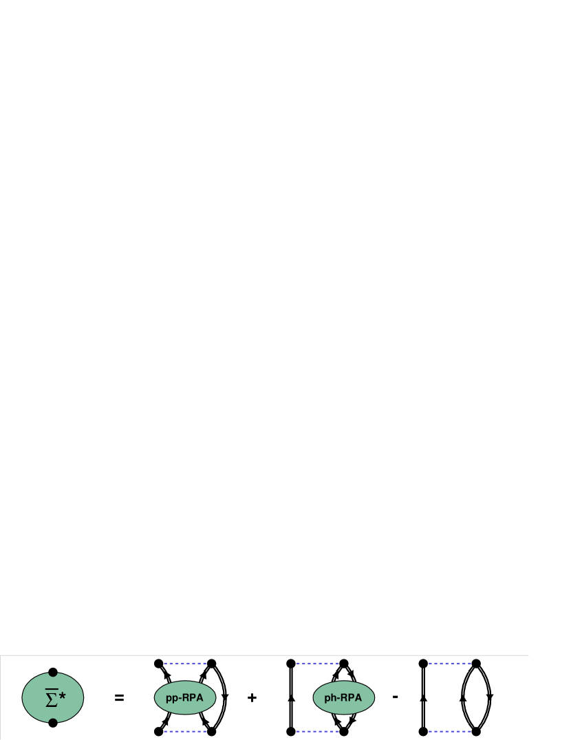
Figure 1: Example of an approximation for the self-energy. Although this approximation contains both ph and pp correlations it would generate incorrect results, due to the need for subtracting the 2nd order term to avoid double counting.

To achieve the inclusion of RPA effects, one needs to pursue a formalism in which the contribution of the pp and ph phonons to the self-energy are summed to all orders, like the example of Fig. 2. This, would avoid the subtraction of the second-order diagram. Such a formalism has been proposed recently barb with the intent of attacking the above issues. In this approximation scheme the effects of both pp (hh) and ph phonons can be evaluated at an RPA level and then summed up to all orders by means of the Faddeev technique Fadd1 ; glock . The treatment of Pauli correlations is also improved over methods that include ph RPA phonons directly in the self-energy, since all exchange terms at the 2p1h level are consistently included.

An issue that one needs to be aware of in the application of the formalism of Faddeev equations is the apparence of spurious solutions. The Faddeev approach consists in substituting the Schödinger equations with a set of three coupled differential equations. As a result, more solutions are generated and about 2/3 of them are spurious. In the general three-body problem, though, the properties of such spurious states are well known and they can be eliminated efficiently Glockle99 . The situation is a little more complex if the Faddeev formalism is applied in a many-body context, with the intent of studying the motion of quasi-particle and quasi-hole excitations. Here, in particular, the fulfillment of closure relations for pp and ph amplitudes is related to the behavior of the spurious Faddeev eigenstates barb . This makes the choice of the interaction boxes to be used a critical problem, since without a proper treatment of this relation the spurious solutions will irremediably mix with the physically meaningful ones.

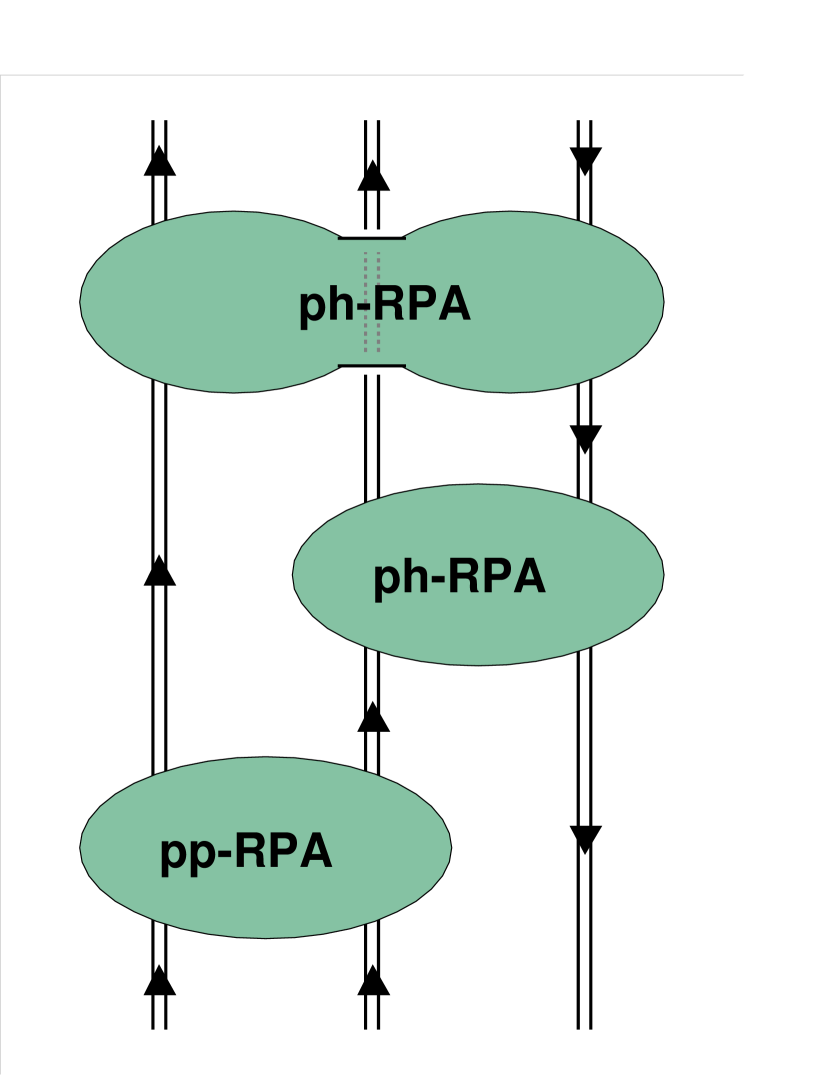
Figure 2: The application of the Faddeev formalism allows to sum the effects of pp (hh) and ph RPA phonons to all orders, generating diagrams like this one. As a result of the all-orders summation, no inconsistent poles will appear in the self-energy.

The Faddeev approach represents a step further with respect to the calculations of Refs. GeurtsO16 ; geurts2h and it is our aim to apply it to the study of one- and two-hole spectral functions of ${}^{16}{\rm O}$. In this contribution, the basic formalism is briefly reviewed. Some details and some technical issues (as the elimination of spurious solutions) are described more completely in Ref. barb and will only be mentioned. The possible implementation of the SCGF scheme is also a key feature of the present formalism and it will also be reviewed in some detail at the end of Sec. II.3

The actual application to the nucleus of ${}^{16}{\rm O}$ is currently under way but has not been completed and will be presented in a future paper. Nevertheless, some preliminary results have been generated for a simplified model and they will be described in the last part, as an example.

II Faddeev formalism for 2h1p and 2p1h motion

The relevant quantities for the study of one- and two-nucleons knockout reactions are the one- and two-hole spectral functions

$$S^{h}_{\alpha}(\omega)~{}=~{}\sum_{k}|{\mbox{$\langle{\Psi^{A-1}_{k}}|$}}c_{\alpha}{\mbox{$|{\Psi^{A}_{0}}\rangle$}}|^{2}\;\delta(\omega+E^{A-1}_{k}-E^{A}_{0})\;,$$ (1)

$$S^{h}_{\alpha\beta}(\omega)~{}=~{}\sum_{k}|{\mbox{$\langle{\Psi^{A-2}_{k}}|$}}c_{\alpha}c_{\beta}{\mbox{$|{\Psi^{A}_{0}}\rangle$}}|^{2}\;\delta(\omega+E^{A-2}_{k-}-E^{A}_{0})\;.$$ (2)

These can be obtained from the diagonal elements of the one- and two- body Green’s function respectively, which in their Lehmann representation take the form fetwa ; AAA

$$g_{\alpha\beta}(\omega)~{}=~{}\sum_{n}\frac{\left({\cal X}^{n}_{\alpha}\right)^{*}\;{\cal X}^{n}_{\beta}}{\omega-\varepsilon^{+}_{n}+i\eta}~{}+~{}\sum_{k}\frac{{\cal Y}^{k}_{\alpha}\;\left({\cal Y}^{k}_{\beta}\right)^{*}}{\omega-\varepsilon^{-}_{k}-i\eta}\;,$$ (3)

and

$$g^{II}_{\mu\nu,\alpha\beta}(\omega)~{}=~{}\sum_{n+}\frac{\left({\cal Z}^{n+}_{\mu\nu}\right)^{*}{\cal Z}^{n+}_{\alpha\beta}}{\omega-\varepsilon^{\Gamma+}_{n+}+i\eta}~{}-~{}\sum_{k-}\frac{{\cal Z}^{k-}_{\mu\nu}\left({\cal Z}^{k-}_{\alpha\beta}\right)^{*}}{\omega-\varepsilon^{\Gamma-}_{k-}-i\eta}\;.$$ (4)

In Eq. (3), ${\cal X}^{n}_{\alpha}={\mbox{$\langle{\Psi^{A+1}_{n}}|$}}c^{{\dagger}}_{\alpha}{\mbox{$|{\Psi^{A}_{0}}\rangle$}}$ (${\cal Y}^{k}_{\alpha}={\mbox{$\langle{\Psi^{A-1}_{k}}|$}}c_{\alpha}{\mbox{$|{\Psi^{A}_{0}}\rangle$}}$) are the spectroscopic amplitudes for the excited states of a system with $A+1$ ($A-1$) particles and the poles $\varepsilon^{+}_{n}=E^{A+1}_{n}-E^{A}_{0}$ ($\varepsilon^{-}_{k}=E^{A}_{0}-E^{A-1}_{k}$) correspond to the excitation energies with respect to the $A$-body ground state. Completely analogous definitions are employed in Eq. (4) for the transition amplitudes and excitation energies related to the states of a system with $A+2$ ($A-2$) particles.

In the nuclear case, a strong coupling exists between the sp degrees of freedom and both collective low-lying states as well as high-lying states. The latter coupling is related to the strong short-range repulsion in the nuclear force. The resulting fragmentation of the sp strength (as observed in experimental data) suggests that this feature must already be included in the description of these couplings. This should be done by expressing the equations used to evaluate the propagators $g_{\alpha\beta}(\omega)$ and $g^{II}_{\mu\nu,\alpha\beta}(\omega)$ in terms of the solution $g_{\alpha\beta}(\omega)$ itself. This self-consistency feature also emerges in an exact formulation, involving the coupling to two-, three- and $A$-body propagators, which can be derived using the equation of motion method masch .

Keeping in mind this approach, we compute $g_{\alpha\beta}(\omega)$ as a solution of the Dyson equation

$$g_{\alpha\beta}(\omega)~{}=~{}g^{(0)}_{\alpha\beta}(\omega)~{}+~{}g^{(0)}_{\alpha\gamma}(\omega)\Sigma^{\star}_{\gamma\delta}(\omega)g_{\delta\beta}(\omega)\;,$$ (5)

where $\Sigma^{\star}_{\alpha\beta}(\omega)$ is the irreducible self-energy. Here and in the following, sums over repeated indices are implied.

By considering the equation of motion for $g_{\alpha\beta}(\omega)$, one obtains that $\Sigma^{\star}_{\alpha\beta}(\omega)$ can be written as the sum of two terms

$$\Sigma^{\star}_{\alpha\beta}(\omega)~{}=~{}\Sigma^{HF}_{\alpha\beta}~{}+~{}\frac{1}{4}\,V_{\alpha\lambda,\mu\nu}~{}R_{\mu\nu\lambda,\gamma\delta\varepsilon}(\omega)~{}V_{\gamma\delta,\beta\varepsilon}\;,$$ (6)

where $\Sigma^{HF}_{\alpha\beta}$ represents the Hartree-Fock part of the self-energy, which can be computed straightforwardly from the solution $g_{\alpha\beta}(\omega)$ itself. The $V_{\alpha\lambda,\mu\nu}$ represent the antisymmetrized matrix elements of the residual interaction.

The non trivial element to be inserted in the calculation is the propagator $R_{\mu\nu\lambda,\gamma\delta\varepsilon}(\omega)$, appearing in the last term of Eq. (6), which describe the motion of excitations consisting of at least two-particle–one-hole (2p1h) or 2h1p states. It contains the sum of all six points diagrams that are one-particle irreducible, i.e. that cannot be separated by cutting a single line.

In general, $R_{\mu\nu\lambda,\gamma\delta\varepsilon}(\omega)$ is the solution of a Bethe-Salpeter type equation involving propagators depending on four times (i.e. three energies) as well as four- and six- point kernels Win72 . This is appears too complex to be solved numerically and one needs to find an appropriate approximation for the propagator $R_{\mu\nu\lambda,\gamma\delta\varepsilon}(\omega)$. The formalism proposed in Ref. barb aims to compute this object keeping the effects of RPA phonons but at the same time restricting oneself to equations involving only two-times propagators, thus producing a set of equations that one can deal with. This is achieved by applying the Faddeev equations technique.

Also, the resulting formalism splits up in two separate expansions for the 2p1h and the 2h1p components. Although the hole spectral function is of primary interest for comparison with experimental data, it must be stressed that both 2p1h and 2h1p components are needed to generate the self-consistent solution for the sp propagator. Since the formalism involved is the same for both components, we will describe only the forward-going (2p1h) expansion in the rest of this section. The equations for the 2h1p case are completely analogous.

II.1 Faddeev equations

As a convention, we assume that the first two lines propagating through the expansion of $R_{\mu\nu\lambda,\gamma\delta\varepsilon}(\omega)$ represent particle excitations while the last represents a hole, as in Fig. 2. Following standard notation in the literature JoachBk , the i-th Faddeev component $R^{(i)}_{\mu\nu\lambda,\alpha\beta\gamma}$ will represent the sum of all diagrams ending with an interaction between legs $j$ and $k$, with $(i,j,k)$ cyclic permutations of $(1,2,3)$. Obviously, the component $R^{(3)}$ refer to the interactions in the pp channel, while the two components $R^{(1)}$ and $R^{(2)}$ will refer to the interaction between a particle and a hole. The last two are trivially related to each other by the exchange of the first two indices.

Also, for reasons to be mentioned in the next subsection, the $R^{(i)}$ need to be redefined in such a way that their matrix elements also depend on the indices ($n$, $n^{\prime}$, $k$), which label the fragments of the external propagator lines (compare with the definitions below Eq. (3) ). This implies that the eigenvalue equations will involve summations on both the sp indices ($\alpha$, $\beta$, $\gamma$) and the ones corresponding to the fragmentation, ($n_{\alpha}$, $n_{\beta}$, $k_{\gamma}$). The 2p1h propagator and its Faddeev components are recovered only at the end of calculations by summing the solutions over all values of ($n_{\alpha}$, $n_{\beta}$, $k_{\gamma}$) and ($n_{\mu}$, $n_{\nu}$, $k_{\lambda}$).

Putting together all the above ingredients, the resulting approximation to the Faddeev equations can be rewritten in a way where all the propagators involved depend only on one energy variable (or two time variables). The 2p1h part of this expansion can be written as follows

$$R^{(i)}_{\mu n_{\mu}\nu n_{\nu}\lambda k_{\lambda},\alpha n_{\alpha}\beta n_{\beta}\gamma k_{\gamma}}(\omega)$$ (7)

$$= \frac{1}{2}\left({G^{0}}^{>}_{\mu n_{\mu}\nu n_{\nu}\lambda k_{\lambda},\alpha n_{\alpha}\beta n_{\beta}\gamma k_{\gamma}}(\omega)-{G^{0}}^{>}_{\nu n_{\nu}\mu n_{\mu}\lambda k_{\lambda},\alpha n_{\alpha}\beta n_{\beta}\gamma k_{\gamma}}(\omega)\right)$$

$$+~{}{G^{0}}^{>}_{\nu n_{\nu}\mu n_{\mu}\lambda k_{\lambda},\mu^{\prime}n_{\mu}^{\prime}\nu^{\prime}n_{\nu}^{\prime}\lambda^{\prime}k_{\lambda}^{\prime}}(\omega)~{}\Gamma^{(i)}_{\nu^{\prime}n_{\nu}^{\prime}\mu^{\prime}n_{\mu}^{\prime}\lambda^{\prime}k_{\lambda}^{\prime},\mu^{\prime\prime}n_{\mu}^{\prime\prime}\nu^{\prime\prime}n_{\nu}^{\prime\prime}\lambda^{\prime\prime}k_{\lambda}^{\prime\prime}}(\omega)~{}$$

$$~{}~{}~{}\times~{}\left(R^{(j)}_{\mu^{\prime\prime}n_{\mu}^{\prime\prime}\nu^{\prime\prime}n_{\nu}^{\prime\prime}\lambda^{\prime\prime}k_{\lambda}^{\prime\prime},\alpha n_{\alpha}\beta n_{\beta}\gamma k_{\gamma}}(\omega)~{}+~{}R^{(k)}_{\mu^{\prime\prime}n_{\mu}^{\prime\prime}\nu^{\prime\prime}n_{\nu}^{\prime\prime}\lambda^{\prime\prime}k_{\lambda}^{\prime\prime},\alpha n_{\alpha}\beta n_{\beta}\gamma k_{\gamma}}(\omega)\right)\;,~{}i=1,2,3~{}.$$

In Eq. (7), ${G^{0}}^{>}$ is the forward-going part of the 2p1h propagator for three dressed but noninteracting lines. Using the notations introduced after Eq. (3) we have

$${G^{0}}^{>}_{\mu n_{\mu}\nu n_{\nu}\lambda k_{\lambda},\alpha n_{\alpha}\beta n_{\beta}\gamma k_{\gamma}}(\omega)~{}=~{}\delta_{n_{\mu},n_{\alpha}}\;\delta_{n_{\nu},n_{\beta}}\;\delta_{k_{\lambda},k_{\gamma}}~{}\frac{\left({\cal X}^{n_{\mu}}_{\mu}{\cal X}^{n_{\nu}}_{\nu}{\cal Y}^{k_{\lambda}}_{\lambda}\right)^{*}\;{\cal X}^{n_{\alpha}}_{\alpha}{\cal X}^{n_{\beta}}_{\beta}{\cal Y}^{k_{\gamma}}_{\gamma}}{\omega-(\varepsilon^{+}_{n_{\alpha}}+\varepsilon^{+}_{n_{\beta}}-\varepsilon^{-}_{k\gamma})+i\eta}\;.$$ (8)

The Faddeev vertices $\Gamma^{(i)}_{\nu^{\prime}n_{\nu}^{\prime}\mu^{\prime}n_{\mu}^{\prime}\lambda^{\prime}k_{\lambda}^{\prime},\mu^{\prime\prime}n_{\mu}^{\prime\prime}\nu^{\prime\prime}n_{\nu}^{\prime\prime}\lambda^{\prime\prime}k_{\lambda}^{\prime\prime}}(\omega)$ contain the collective excitations in the pp and ph channels and can be evaluated in RPA, as explained in the next subsection.

Once the Faddeev equations are solved and the usual representation of the Faddeev components $R^{(i)}_{\mu\nu\lambda,\alpha\beta\gamma}$ is recovered by summing over the indices ($n_{\alpha}$, $n_{\beta}$, $k_{\gamma}$) and ($n_{\mu}$, $n_{\nu}$, $k_{\lambda}$), the complete 2h1p propagator can be obtained as the sum of all the components:

$$R_{\mu\nu\lambda,\alpha\beta\gamma}(\omega)~{}=~{}\sum_{i=1,2,3}R^{(i)}_{\mu\nu\lambda,\alpha\beta\gamma}(\omega)~{}-~{}\frac{1}{2}\left({G^{0}}^{>}_{\mu\nu\lambda,\alpha\beta\gamma}(\omega)-{G^{0}}^{>}_{\nu\mu\lambda,\alpha\beta\gamma}(\omega)\right)\;,$$ (9)

The free forward-going propagator ${G^{0}}$ was already included in the Eqs. (7) and therefore is to be subtracted in Eq. (9) to avoid double countings. It must be stressed though that this subtraction does not generate any inconsistencies in the self-energy, as it was the case for the approximation of Fig. 1. Rather, this subtraction is required to exactly cancel similar, troublesome, terms that are included in the single Faddeev components.

II.2 Faddeev vertices

The interaction matrices $\Gamma^{(pp)}_{\mu\nu,\alpha\beta}(\omega)$ for the pp channel and $\Pi^{(ph)}_{\mu\nu,\alpha\beta}(\omega)$ for the ph channel, are obtained by solving the ladder equation in the Dressed RPA (DRPA) scheme, which employs dressed propagators as they are obtained by solving the Dyson equation (5).

For the pp case, the DRPA equation is graphically depicted in Fig. 3. The gamma matrix $\Gamma^{(pp)}_{\mu\nu,\alpha\beta}(\omega)$ obtained in this way is the generalization of the two-body T-matrix for two nucleons and represents our approximation for the two-particle propagator of Eq. (4), when the external legs are amputated. Completely analogous considerations apply to the ph interaction matrix $\Pi^{(ph)}_{\mu\nu,\alpha\beta}(\omega)$.

The RPA phonons generated in this way depend on dressed propagators and can be included in the Faddeev formalism outlined above. It is worth noting that discarding the last diagram on the right hand side of Fig. 3, and in the corresponding ph counterpart, the whole formalism reduces to the TDA expansion of Ref. GeurtsO16 .

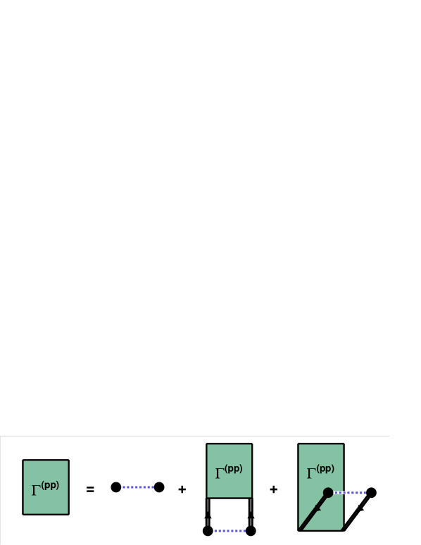
Figure 3: DRPA equation for the $\Gamma^{(pp)}$ matrix.

The vertices to be employed in the Faddeev equations (7) will consists of the interaction boxes just described to which a freely propagating dressed line is added, as displayed in Fig. 4. The exact formula for the pp channel is as follows:

$$\Gamma^{(3)}_{\mu n_{\mu}\nu n_{\nu}\lambda k_{\lambda},\alpha n_{\alpha}\beta n_{\beta}\gamma k_{\gamma}}(\omega)~{}=~{}{\textstyle{1\over 2}}\frac{\delta_{k_{\lambda},k_{\gamma}}}{\sum_{\sigma}\left|{\cal Y}^{k_{\lambda}}_{\sigma}\right|^{2}}$$

$$\times~{}\left\{V_{\mu\nu,\alpha\beta}~{}+~{}\sum_{n+}\frac{\left(\Delta^{n+}_{\mu\nu}\right)^{*}\Delta^{n+}_{\alpha\beta}}{\omega-(\varepsilon^{\Gamma+}_{n+}-\varepsilon^{-}_{k_{\lambda}})+i\eta}\right.$$ (10)

$$~{}+~{}\left.\sum_{k-}\frac{[\omega-\varepsilon^{+}_{n_{\mu}}-\varepsilon^{+}_{n_{\nu}}-\varepsilon^{+}_{n_{\alpha}}-\varepsilon^{+}_{n_{\beta}}+\varepsilon^{-}_{k_{\lambda}}+\varepsilon^{\Gamma-}_{k-}]\;\Delta^{k-}_{\mu\nu}\left(\Delta^{k-}_{\alpha\beta}\right)^{*}}{(\varepsilon^{\Gamma-}_{k-}-\varepsilon^{+}_{n_{\mu}}-\varepsilon^{+}_{n_{\nu}})(\varepsilon^{\Gamma-}_{k-}-\varepsilon^{+}_{n_{\alpha}}-\varepsilon^{+}_{n_{\beta}})}\right\}\;,$$

were the $\Delta^{n+}$ ($\Delta^{k-}$) amplitudes are computed through the DRPA equation of Fig. 3 and are related to the amplitudes of Eq. (4) by $\Delta^{n+}_{\mu\nu}=V_{\mu\nu,\alpha\beta}\,{\cal Z}^{n+}_{\alpha\beta}$ ($\Delta^{k-}_{\mu\nu}={\cal Z}^{k-}_{\alpha\beta}\,V_{\alpha\beta,\mu\nu}$).

The complication of defining the interaction vertex $\Gamma^{(3)}$ not only in terms of the sp indices but also in terms of the respective fragmentations ($n_{\mu}$, $n_{\nu}$, $k_{\lambda}$) and ($n_{\alpha}$, $n_{\beta}$, $k_{\gamma}$) is a consequence of the two main requirements imposed: that is, $\Gamma^{(3)}$ has to depend on only two times and the free line added in Fig. 4 must be a dressed propagator. As it can be seen from Eq. (10), the energy poles $\varepsilon^{-}_{k_{\lambda}}$, relative to the fragments of this line, appear in the equation mixed with the corresponding poles of the $\Gamma^{(pp)}_{\mu\nu,\alpha\beta}(\omega)$’s phonons. This situation couldn’t be handled without the above prescription DRPApaper ; barb . Instead, with this procedure it is still possible to write an expression for the diagrams of Fig. 4 in the form ${G^{0}}^{>}(\omega)\;\Gamma^{(3)}(\omega)\;{G^{0}}^{>}(\omega)$ or, equivalently, to write the Faddeev equations (7).

As a last remark, we note that the last term on the right hand side of Eq. (10) comes from the last diagram of Fig. 4. This term contains large energy denominators and it is expected to give relatively small contributions. Nevertheless, it can be proved that it is essential to include it in order to impose the appropriate behavior of the spurious solutions generated by the Faddeev equations (and eventually to discard them) barb . Thus also this diagram needs to be kept.

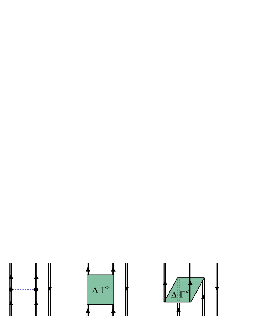
Figure 4: Here $\Delta\Gamma^{>}$ and $\Delta\Gamma^{<}$ are the forward- and backward-going part of the energy dependent contribution to the pp DRPA vertex (4). The contribution of these three diagrams can be factorized in an expression of the form ${G^{0}}^{>}\;\Gamma^{(3)}\;{G^{0}}^{>}$ only after having redefined the propagators ${G^{0}}^{>}$ and $\Gamma^{(3)}$ to depend also on the particle and hole fragmentation indices ($n$,$n^{\prime}$,$k$). The last diagram has a smaller effect on the physical solutions of the problem, although it is essential for the elimination of spurious solutions.

II.3 Self-consistent Scheme

The set of Faddeev equations (7), together with the expressions (5) and (6), furnish a scheme in which one- and two-body spectral functions can be evaluated in terms of an already dressed single-particle Green’s function. This allows the possibility of including, already from the start, the features of the single-particle motion that go beyond a mean-field description. Once such features are included in the input propagator, their effects on the one- and two-body motion will be automatically included in the calculations. It is important to observe that the expansion of the irreducible propagator $R_{\mu\nu\lambda,\gamma\delta\varepsilon}(\omega)$ in Eq. (6), derived employing the equation of motion, is given in terms of the real one-body propagator. Thus, in principle, it is the exact solution of the many-body problem that is supposed to be employed in the Faddeev calculations described above.

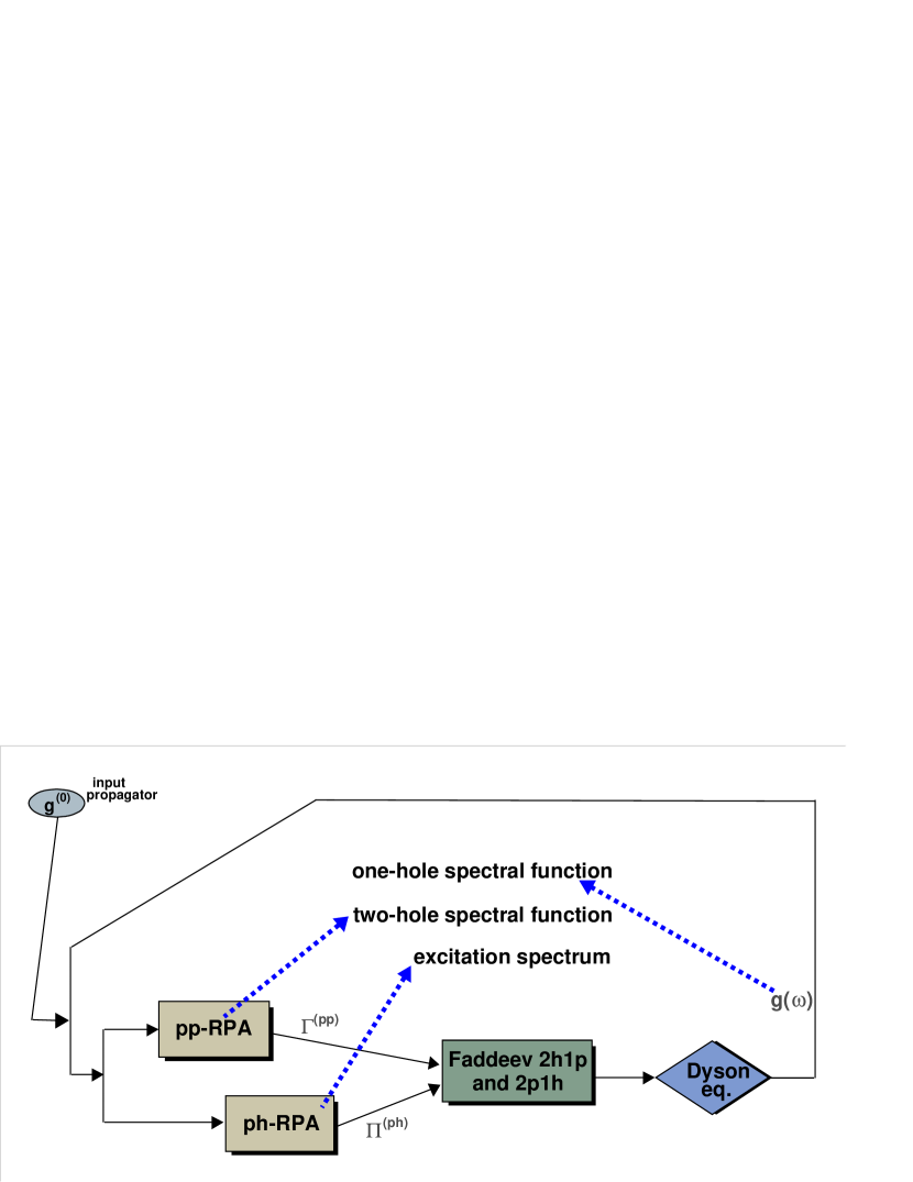
Figure 5: Iteration scheme used to reach self-consistency between the input propagator and the result of the Dyson equation. At each iteration new approximations for the one- and two- body propagators (3) and (4) are obtained.

The approach of self-consistent Green’s function theory consists in starting with an approximation for the input Green’s function (usually an Hartee-Fock propagator or other independent particle model). From this, the pp (hh), the ph and the Faddeev propagators can be evaluated with the formalism described. Then, the solution of the Dyson Eq. (5) will give a better approximation of the s.p. propagator, that can be employed in the second calculation. As Shown in Fig. 5, the whole procedure is iterated many times until consistency is found between two successive solutions (i.e. between the input propagator and the solution that it generates).

The attractive feature of this procedure is not only restricted to the fact that the effects of fragmentation are included in the calculations. But also, expressions for the one- and two-hole motion and the ph phonons (which give information on the excitation spectrum of the system) are generated all at the same time, the relative effects of each one on the others being taken into account.

Obviously, the exact form of the single-particle propagator is very complex, containing many poles and a continuum. Such richness of details cannot be easily included in the above calculation. In our case, though, we are interested in the low energy behavior of the single-particle motion and the few poles that contain the main sp strength are expected to be much more relevant than the others. One possible prescription to limit the number of poles in the input propagator at each iteration consists in keeping only the most significant peaks and collapsing all the others in an effective pole. This procedure was already employed in applying the SCGF method to the study of pairing in superfluid nuclei jyuan ; wim99 .

The effects coming from short-range correlations, can be taken into account by substituting the bare NN potential $V_{\alpha\beta,\gamma\delta}$ with a G-matrix interaction. In the same way, the effects of short-range interaction can be included in the two-hole spectral function by adding the relative defect functions as done in Ref. geurts2h ; geueepp .

III Quadrupole-plus-Pairing Model

The implementation of the Faddeev RPA formalism available at the moment allows us to make a test with a simplified model for the ${}^{16}{\rm O}$ nucleus. We considered a model space consisting of harmonic oscillator wave functions up to four major closed shells ($2p$ and $1f$ states) plus a $g_{9/2}$ single particle state. Within this space, we choose a so called “pairing-plus-quadrupole” Hamiltonian schuckbook , in which one a body potential $\hat{U}$ is employed to generate the correct single-particle energies and the residual interaction in composed of a quadrupole-quadrupole $\hat{V}_{\cal Q}$ and a pairing $\hat{V}_{\cal P}$ term:

$$\hat{H}~{} = ~{}\hat{U}~{}+~{}\hat{V}_{\cal Q}~{}+~{}\hat{V}_{\cal P}$$ (11)

$$= ~{}\sum_{\alpha}\varepsilon^{0}_{\alpha}~{}c^{{\dagger}}_{\alpha}c_{\alpha}~{}+~{}g_{{}_{\cal Q}}~{}:\hat{Q}^{{\dagger}}\hat{Q}:~{}+~{}g_{{}_{\cal P}}~{}\hat{P}^{{\dagger}}\hat{P}\;,$$

where $\hat{P}~{}\equiv\sum_{\alpha}c_{\alpha}c_{\bar{\alpha}}$ and $\hat{Q}~{}\equiv\sum_{\alpha,\beta}{\mbox{$\langle{\alpha}|$}}r^{2}Y_{2,m}(\Omega_{r}){\mbox{$|{\beta}\rangle$}}c^{{\dagger}}_{\alpha}c_{\beta}$ are the pairing and the quadrupole operators, the symbol “$:$” represents the normal ordering and $\bar{\alpha}$ is the time reversal of state $\alpha$. An oscillator parameter of $b~{}=~{}1.76~{}fm$ was used in computing the quadrupole matrix elements. Both $\hat{V}_{\cal P}$ and $\hat{V}_{\cal Q}$ are independent of the spin and isospin degrees of freedom.

The values of $\varepsilon^{0}_{\alpha}$ for all the sp states were computed in Ref. GeurtsO16 in a Brueckner-Hartree-Fock calculation, based on a G-matrix interaction CALGM derived from the Bonn-C potential bonnc . The $\varepsilon^{0}_{\alpha}$ used here are are taken from that reference but with some slight modification of the levels close to the Fermi energy, in order to roughly reproduce the experimental missing energies in the Faddeev RPA calculation. The exact values employed here are given in table 1.

Table 1: Single particle energies $\varepsilon^{0}_{\alpha}$ and interaction strengths used in Eq. (11). The sp energies were computeded from Ref. GeurtsO16 , while $g_{{}_{\cal Q}}$ and $g_{{}_{\cal P}}$ were fitted to roughly reproduce the excitation energy of the $3^{-}$ ph phonon.

$\alpha$		$\;\;1s_{1/2}\;\;$	$\;\;1p_{1/2}\;\;$	$\;\;1p_{3/2}\;\;$	$\;\;1d_{5/2}\;\;$	$\;\;2s_{1/2}\;\;$	$\;\;1d_{3/2}\;\;$	$\;\;1f_{7/2}\;\;$	$\;\;2p_{3/2}\;\;$	$\;\;1f_{5/2}\;\;$	$\;\;2p_{1/2}\;\;$	$\;\;1g_{9/2}\;\;$
$\varepsilon^{0}_{\alpha}(MeV)$		$-35.0$	$-18.2$	$-9.3$	$-1.8$	$-0.1$	$4.4$	$17.4$	$16.0$	$23.5$	$17.7$	$30.0$
			$g_{{}_{\cal Q}}=-1.14\;MeV/fm^{4}$					$g_{{}_{\cal P}}=+15.0\;MeV$

The remaining two parameters, $g_{{}_{\cal Q}}$ and $g_{{}_{\cal P}}$, were fitted to other experimental energies. In particular, $g_{{}_{\cal Q}}$ was chosen to roughly reproduce the $3^{-}$ phonon of ${}^{16}{\rm O}$, while $g_{{}_{\cal P}}$ was fitted aiming to reproduce the experimental missing energy of the ${}^{14}{\rm C}$ ground state. The latter was found to be not very sensitive and was then fixed to the value given in table 1.

Table 2: Results for hole spectroscopic factors of the main $p_{1/2}$ and $p_{3/2}$ peaks, obtained with Hamiltonian (11).

			TDA		RPA
	$p_{1/2}$		.632		.588
	$p_{3/2}$		.668		.647

Using the Hamiltonian (11), the self-energy was computed employing the Faddeev formalism with pp (hh) and ph phonons evaluated in both TDA and RPA schemes. As already noticed, the TDA approximation was already employed in the calculation of Ref. GeurtsO16 .

As seen from table 2, the results obtained for the $p_{1/2}$ and $p_{3/2}$ spectroscopic factors are 4-5 % smaller in the RPA case and seem to go in the expected way.

It’s worth to recall that the results from this model have been obtained within a single iteration, without the effects of short-range correlations and with a oversimplified interaction. Thus the values obtained for the absolute spectroscopic factors are not really meaningful and are expected to change significantly in a realistic calculation. Self-consistency can play a relevant role too.

Nevertheless, a comparison between the results obtained in TDA and RPA calculation seems reasonable and can give some idea of the relative importance of RPA effects.

IV Summary

The present theoretical description of the distribution of spectroscopic strength at low energies lacks important ingredients for a successful comparison with experimental data. One of these ingredients is a proper description of the coupling of sp motion to low-lying collective modes that are present in the system. Recent calculations for ${}^{16}{\rm O}$ GeurtsO16 , for example, only include a TDA description of these collective modes. This contribution outlines a new method that has been proposed recently barb that aims to study the influence of pp and ph RPA correlations on the sp propagator for a system with a finite number of fermions. This method is formulated in the context of SCGF theory by evaluating the nucleon self-energy in terms of the 2p1h and 2h1p propagators. The description of the 2p1h (or 2h1p) excitations has been studied by using the Faddeev formalism, which is usually applied to solve the three-body problem. As mentioned in the text, the detailed choice of the form of the interaction matrices as well as the formulation of the problem are imposed by practical issues, like the existence of spurious solutions.

It should be noted that the Faddeev approach outlined here, has also the advantage that it can be naturally extended to the inclusion of more complicated excitations like the extended DRPA DRPApaper .

The application of this formalism is underway for the nucleus of ${}^{16}{\rm O}$. Although no physically meaningful results have been obtained yet, the Faddeev RPA equations have been applied to a simple model, demonstrating the feasibility of these calculations. The results obtained with this model yield somewhat stronger quenching of the $p_{1/2}$ and $p_{3/2}$ spectroscopic factors when RPA correlations are included, thus going in the expected direction.

A realistic self-consistent calculation in which a G-matrix derived from realistic interaction is employed is underway and the results will be reported elsewhere.

References

- (1) A. E. L. Dieperink and P. de Witt Huberts, Ann. Rev. Nucl. Part. Sci. 40, 239 (1990).
- (2) I. Sick and P. de Witt Huberts, Commun. Nucl. Part. Phys. 20, 177 (1991).
- (3) L. Lapikás, Nucl. Phys. A553, 297c (1993).
- (4) M. Leuschner et al., Phys. Rev. C 49, 955 (1994).
- (5) J. Udìas et al., nucl-th/010138, to be published on Phys. Rev. C. and contribution to this workshop.
- (6) M. Radici, S. Boffi, S. C. Pieper, and V. R. Pandharipande, Phys. Rev. C 50, 3010 (1994).
- (7) H. Müther and W. H. Dickhoff, Phys. Rev. C 49, R17 (1994).
- (8) A. Faborcini and G. Co’, Phys. Rev. C 63, 044319 (2001).
- (9) D. Van Neck, M.Waroquier, A. E. L. Dieperink, S C. Pieper, and V. R. Pandharipande, Phys. Rev. C 57, 2308 (1998).
- (10) O. Benhar, A. Fabrocini, S. Fantoni, Phys. Rev. C 41, R24 (1990).
- (11) A. Fabrocini, contribution to this workshop.
- (12) W. J. W. Geurts, K. Allaart, W. H. Dickhoff, and H. Müther, Phys. Rev. C 53, 2207 (1996).
- (13) P. Czerski, W. H. Dickhoff, A. Faessler, and H. Müther, Phys. Rev. C 33, 1753 (1986).
- (14) W. J. W. Geurts, K. Allaart, W. H. Dickhoff, and H. Müther, Phys. Rev. C 54, 1144 (1996).
- (15) C. Giusti, F. D. Pacati, K. Allaart, W. J. W. Geurts, W. H. Dickhoff, and H. Müther, Phys. Rev. C 57, 1691 (1998).
- (16) H. Müther and P. Sauer, in Computational Nuclear Physics ed. by K.-H. Langanke, et al. (Springer Berlin, 1993).
- (17) C. J. C. Onderwater et al., Phys. Rev. Lett. 78, 4893 (1997).
- (18) C. J. C. Onderwater et al., Phys. Rev. Lett. 81, 2213 (1998).
- (19) M. O. Distler, contribution to this workshop.
- (20) G. Rosner, Prog. Part. Nucl. Phys. 44, 99 (2000)
- (21) G. A. Rijsdijk, K. Allaart, and W. H. Dickhoff, Nucl. Phys. A550, 159 (1992).
- (22) C. Barbieri, W. H. Dickhoff, Phys. Rev. C 63, 034313 (2001).
- (23) L. D. Faddeev, Zh. Éksp. Theor. Fiz. 39, 1459 (1961) [Sov. Phys. JETP 12, 1014 (1961)].
- (24) W. Glöckle, The Quantum Mechanical Few-Body Problem (Springer, Berlin, 1983).
- (25) P. Navrátil, B. R. Barrett, and W. Glöckle, Phys. Rev. C 59, 611 (1999).
- (26) A. L. Fetter and J. D. Walecka, Quantum Theory of Many-Particle Physics (McGraw-Hill, New York, 1971).
- (27) A. A. Abrikosov, L. P. Gorkov and I. E. Dzyaloshinski, Methods of Quantum Field Theory in Statistical Physics (Dover, New York, 1975).
- (28) P. C. Martin and J. Schwinger, Phys. Rev. 115, 1342 (1959).
- (29) J. Winter, Nucl. Phys. A194, 535 (1972).
- (30) C. J. Joachain Quantum Collision Theory, (North-Holland, Amsterdam, 1975).
- (31) J. Yuan, Ph.D. thesis, Washington University, St. Louis, 1994.
- (32) W. H. Dickhoff, in Nuclear Methods and the Nuclear Equation of State, ed. M. Baldo (World Scientific, Singapore, 1999) p. 326.
- (33) P. Ring and P. Schuck, The Nuclear Many-body Problem (Springer, New York, 1980).
- (34) R. Machleidt, Adv. Nucl. Phys. 19, 191 (1989).
- (35) W. J. W. Geurts, K. Allaart, and W. H. Dickhoff, Phys. Rev. C 50, 514 (1994).