Analytical E1 strength functions of two–neutron halo nuclei: the $\@@nuc{6}{He}$ example

Abstract

An analytical model is developed to study the spectra of electromagnetic dissociation of two–neutron halo nuclei without precise knowledge about initial and final states. Phenomenological three–cluster bound state wave functions, reproducing the most relevant features of these nuclei, are used along with no interaction final states. The $\@@nuc{6}{He}$ nucleus is considered as a test case, and a good agreement with experimental data concerning the shape of the spectrum and the magnitude of the strength function is found.

, and

1 Introduction

Coulomb excitation reactions serve as one of the most powerful tools for investigating excited states of nuclei. An appealing feature of these reactions is the clear understanding of the interaction mechanism. In particular, electromagnetic dissociation (EMD) of halo nuclei has revealed an anomalously large cross sections due to accumulation of electric dipole (E1) strength at low energy. The first attempts to interpret the phenomenon of low–energy excitations addressed a notion of the so–called soft dipole resonance [1, 2, 3, 4, 5]. However, it is still an open question whether this is a true resonant state, which is being observed through the E1 excitation. For example, intensive studies of the one–neutron halo nucleus $\@@nuc{11}{Be}$ have shown a very significant enhancement of the E1 strength just above the $\@@nuc{10}{Be}$$\,+\,$n threshold where there are no resonances in $\@@nuc{11}{Be}$. For $\@@nuc{6}{He}$ several different three–body approaches [3, 6, 7, 8, 9] agree that there is no low–lying $1^{-}$ resonant state in the continuum. An alternative way to explain the accumulation of E1 strength would be to consider a direct breakup, where the final states are continuum states without a resonant state. In the direct breakup mechanism, low–energy dipole excitations occur as a natural consequence of the small binding energy or correspondingly of the large distance between the charge and the center of mass (CM) of a halo nucleus. In this way the E1 strength function of the one–neutron halo nucleus $\@@nuc{11}{Be}$ can be explained using a simple two–body model with a Yukawa wave function (WF) for the initial state and plane waves in the final state [10, 11]. However, for two–neutron halo nuclei, like $\@@nuc{6}{He}$, $\@@nuc{11}{Li}$, and $\@@nuc{14}{Be}$, a three–body picture is more appropriate but also more complicated. Microscopic three–cluster calculations of the E1 strength function were performed for, e.g., $\@@nuc{6}{He}$ [9, 12]. However, many difficulties and questions caused by incomplete knowledge of the cluster dynamics are still to be resolved. In the present paper we develop an alternative approach. We construct phenomenological three–cluster bound state WFs of two–neutron halo nuclei that behave correctly at large intercluster distances, reproduce the nuclear sizes, and incorporate the main features of the underlying three–body structure. No interaction three–body WFs are used to describe the breakup final states. The model allows an analytic calculation of the strength functions and can serve as a helpful tool to predict the Coulomb disintegration spectra of a variety of two–neutron halo nuclei. This can help to conduct new experiments and eventually can provide a better understanding of the microscopic structure of halo nuclei. An approach of this type has previously been used by Pushkin et al. [13] and the present work can be viewed as a development of their model.

In the present paper the model is formulated. As a test case the E1 strength function of $\@@nuc{6}{He}$ is studied and compared with the experimental data of Aumann et al. [14]. In a subsequent paper the model will be applied to $\@@nuc{11}{Li}$ and $\@@nuc{14}{Be}$. In Sec. 2 our WFs are described, in Sec. 3 the strength functions are obtained and discussed, and in Sec. 4 some conclusions are presented. Details of the calculation are given in the Appendix.

For further reference we list here conventional formulae concerning the EMD. We consider the case when an initial ground state is the only bound state in a system (note that all known Borromean nuclei possess this property) and all possible final states belong to the continuum. In the framework of first order perturbation theory the energy spectrum for E1 Coulomb excitation can be written as

$$\frac{\d\sigma(\mathrm{E}1)}{\d E}=\frac{N_{\mathrm{E}1}(E^{*})}{\hbar c}\frac{16\pi^{3}}{9}\frac{\mathrm{d}B(\mathrm{E}1)}{\mathrm{d}E}.$$ (1)

Here $E^{*}$ is the excitation energy, $E^{*}=E_{0}+E$, where $E_{0}$ is the binding energy, and $E$ is thus the continuum energy, $\d B(\mathrm{E}1)/\d E$ is the dipole strength function, and $N_{\mathrm{E}1}(E^{*})$ [15, 16] is the spectrum of virtual photons (where the actual number $\d n$ of virtual photons equals to $N_{\mathrm{E}1}(E^{*})(E^{*})^{-1}\d E$). Since the spectrum of virtual photons peaks at low energies, the Coulomb excitation to low–lying states is favored as far as there exists a low–energy contribution to the dipole strength.

The E1 strength function can be written as

$$\frac{\mathrm{d}B(\mathrm{E}1)}{\mathrm{d}E}=\frac{1}{2J_{i}+1}\sum_{M_{i}}\sum_{\mu=-1,0,1}\int\d\tau_{f}\left|\langle f|\mathcal{M}(\mathrm{E}1,\mu)|i;J_{i}M_{i}\rangle\right|^{2}\delta\left(E_{f}-E\right).$$ (2)

Here $\d\tau_{f}$ is the phase space element for final states, $\vec{\mathcal{M}}(\mathrm{E}1)$ is the dipole operator, and $|i\rangle$, $|f\rangle$ are the initial state and the final states in the CM subsystem which are normalized as follows

$$\langle i|i\rangle=1,\qquad\langle f|f^{\prime}\rangle=\delta(\tau_{f}-\tau_{f}^{\prime}).$$ (3)

In the case when discrete quantum numbers enter the labelling of continuum final states the $\delta$–function notation adopted above implies inclusion of $\delta$–symbols. Similarly, the notation $\int\d\tau_{f}$ in Eq. (2) may imply the inclusion of summation over discrete quantum numbers.

Since halo nuclei exhibit a large degree of clusterization, low–energy excitations will mainly affect relative motion between the $N$ clusters. The corresponding cluster E1 operator is

$$\vec{\mathcal{M}}(\mathrm{E}1)=\sqrt{\frac{3}{4\pi}}\sum_{i=1}^{N}eZ_{i}(\vec{r}_{i}-\vec{R}_{\mathrm{cm}}),$$ (4)

where $\vec{r_{i}}$ are the cluster positions, and $\vec{R}_{\mathrm{cm}}$ is the position of the CM of the system. In the case of two–neutron halo nuclei only the core will contribute in Eq. (4).

By summing the strength over all final states one obtains sum rules for the process. In particular, the non–energy–weighted cluster sum rule reads in our case as

$$\int_{0}^{\infty}\frac{\d B(\mathrm{E}1)}{\d E}\d E=\frac{3}{4\pi}Z_{\mathrm{c}}^{2}e^{2}\langle r_{\mathrm{c}}^{2}\rangle,$$ (5)

where $Z_{\mathrm{c}}$ is the charge of the core, $r_{\mathrm{c}}$ is the distance between the core and the CM of the whole system, and the average value is calculated over the ground state WF.

2 Wave functions and transition matrix elements

In the present analysis we adopt the three–body model description of two–neutron halo nuclei. The cluster part of the bound state WF, in the CM subsystem, is written as an expansion over hyperspherical harmonics (HH) (see e.g. [17])

$$\Psi\left(\vec{x},\vec{y}\right)=\rho^{-5/2}\sum_{KLSl_{x}l_{y}}\chi_{KLS}^{l_{x}l_{y}}\left(\rho\right)\left[\Gamma_{KL}^{l_{x}l_{y}}\left(\Omega_{5}\right)\otimes\theta_{S}\right]_{JM}.$$ (6)

Here $\{\vec{x},\vec{y}\}$ is the set of Jacobi coordinates (17), and $\{\rho,\Omega_{5}\}$ are the corresponding hyperspherical coordinates. The quantity $\rho=\left(x^{2}+y^{2}\right)^{1/2}$ is the hyperradius, and $\{\Omega_{5}\}$ denotes collectively five angles parametrizing a hypersphere with $\rho=\mathrm{const}$. We use below that

$$\d\vec{x}\d\vec{y}=\rho^{5}\d\rho\d\Omega_{5}.$$ (7)

The HH, $\Gamma_{KLM_{L}}^{l_{x}l_{y}}\left(\Omega_{5}\right)$, form an orthonormalized complete set. Harmonics with the orbital quantum numbers $L,M_{L}$ are coupled with spin functions of two neutrons $\theta_{SM_{S}}$ to the total momentum $J,M$. The other quantum numbers labelling the HH are the Jacobi orbital momenta $l_{x}$, $l_{y}$, and the hypermomentum $K$. Since the WF (6) should be antisymmetric with respect to the valence neutrons it includes only terms with even $(l_{x}+S)$. More details can be found in the Appendix.

For Borromean systems, having no bound subsystems, which include two neutrons as constituents, the hyperradial functions entering the expansion (6) behave asymptotically as (see, e.g., [18])

$$\chi_{\lambda}(\rho)\rightarrow C_{\lambda}\exp(-\kappa_{0}\rho),\qquad\mathrm{as}\quad\rho\rightarrow\infty,$$ (8)

where $\kappa_{0}$ is connected to the binding energy via $E_{0}=(\hbar\kappa_{0})^{2}/(2m)$, and $m$ is the nucleon mass. Thus, for a nucleus with a small binding energy the WF has a long tail which is of importance for peripheral reactions such as EMD. One could choose a phenomenological bound state WF using the normalized hyperradial function

$$\chi^{(1)}(\rho)\equiv\sqrt{2\kappa_{0}}\exp(-\kappa_{0}\rho),$$ (9)

together with the HH from expansion (6) which has a predominant weight. The single free parameter, $\kappa_{0}$, is fixed from the binding energy. Such a model WF, incorporating the $K=0$ HH, has been used in Ref. [13] for the $\@@nuc{11}{Li}$ case and led to an analytic expression for the E1 strength function reproducing well the shape of existing experimental data. The total WF behaves as $\rho^{-5/2}$ for small $\rho$ but it is still normalizable since the singularity cancels with the $\rho^{5}$ factor in the volume element, Eq. (7). However, using this model the WF is overestimated at small $\rho$ and thus the $\sqrt{2\kappa_{0}}$ value is smaller than the true asymptotic constant. This leads to an underestimation of $\langle\rho^{2}\rangle$ and consequently to an underestimation of the size of the system since, in accordance with Eq. (18),

$$\langle R^{2}_{\mathrm{rms}}\rangle=A^{-1}\left[\langle\rho^{2}\rangle+(A-2)\langle R^{2}_{\mathrm{rms}}(\mathrm{core})\rangle\right],$$

where $A$ is the mass number, and the last term represents the intrinsic size of the core.

In our model, to cure this feature, we will be add an extra hyperradial term of the same exponential form to reproduce simultaneously the true asymptotic behavior of the ground state (connected to the binding energy) and its size. The corresponding normalized function is

$$\begin{split}\chi^{(2)}(\rho)&\equiv c\left[\exp(-\kappa_{0}\rho)-\exp(-\kappa_{1}\rho)\right],\\ &\mathrm{where}\quad c=\sqrt{\frac{2\kappa_{0}\kappa_{1}(\kappa_{0}+\kappa_{1})}{(\kappa_{0}-\kappa_{1})^{2}}}.\end{split}$$ (10)

The parameters $\kappa_{0}$ and $\kappa_{1}$ are fixed using experimental values of binding energy and rms radius. With the condition that $\kappa_{1}>\kappa_{0}$ we ensure that the second term decays faster than the first, and thus the correct asymptotics is preserved. Furthermore, the divergence of the total WF at small $\rho$ has been reduced to $\rho^{-3/2}$. The particular form of the function (10) has been chosen to be able to perform the calculations analytically.

We shall retain only one or a few terms in the HH expansion (6). This approximation is motivated by the rapid increase of the multidimensional centrifugal barrier as the hypermoment $K$ increases, see e.g. [17]. The predominant terms in the expansion usually correspond to the lowest possible value of $K$ that is not suppressed by the Pauli principle.

In the $\@@nuc{6}{He}$ case the above approximations lead us to the following normalized, model WF for the initial bound state ($J^{\pi}=0^{+}$)

$$\begin{split}\Psi(\vec{x},\vec{y})=\frac{\chi^{(N)}(\rho)}{\rho^{5/2}}\left\{\left[\sqrt{w_{00}}\Gamma_{000}^{00}\left(\Omega_{5}\right)+\sqrt{w_{20}}\Gamma_{200}^{00}\left(\Omega_{5}\right)\right]\theta_{00}\right.\\ \left.+\sqrt{w_{21}}\left[\Gamma_{21}^{11}\left(\Omega_{5}\right)\otimes\theta_{1}\right]_{J=0}\right\},\qquad\mathrm{where~{}}w_{00}+w_{20}+w_{21}=1.\end{split}$$ (11)

Here $\chi^{(N)}$ is given by Eq. (10) (or alternatively by Eq. (9)). For the HH retained in Eq. (11) realistic hyperradial functions, in the corresponding expansion, behave rather similarly at large $\rho$ of interest, so that the model with hyperradial functions of the same form is permissible. The $\alpha$–N interaction is repulsive in s states due to the Pauli principle, and it is attractive in p states. Because of this the $K=0$ contribution to the WF of $\@@nuc{6}{He}$ is small, and the lowest $K$ value, which is not Pauli suppressed, is $K=2$. From the $K=2$ contributions to the WF, given by the second and third terms in Eq. (11), only the $\Gamma_{200}^{00}$ term involves the s wave NN attraction and at the same time it includes a very large component with the p wave $\alpha$–N attraction. As a result, the term with $\Gamma_{200}^{00}$ should have a predominant weight, and to a first approximation we may keep only this single term. One can also retain all three terms entering Eq. (11) using stable estimates for the weights of the HH components taken from theoretical predictions [17], see Table 1. Similar phenomenological WFs may be constructed for other two–neutron halo nuclei. Explicit expressions for the HH entering the initial state (11) are given in Eq. (23).

In Table 1 parameters of our $\@@nuc{6}{He}$ bound state WFs thus obtained are listed. The experimental values of the two–neutron separation energy $S_{2n}=0.97$ MeV and the rms radius $R_{\mathrm{rms}}=2.50$ fm are adopted for $\Psi_{2}$ and $\Psi_{3}$. The $R_{\mathrm{rms}}=1.79$ fm for the function $\Psi_{1}$ is too small as discussed above.

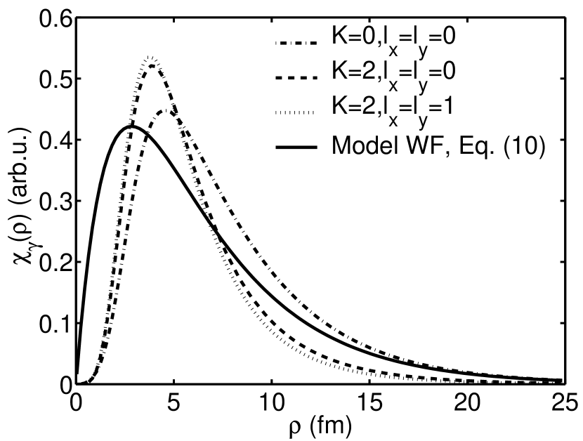
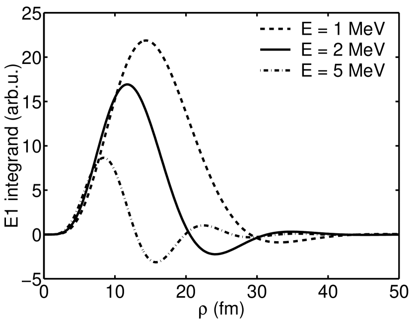
(a)

(b)

Figure 1: (a) The model hyperradial function $\chi^{(2)}$, Eq. (10) (solid line), compared with the three predominant hyperradial functions in expansion (6) obtained from a microscopic three–body calculation of $\@@nuc{6}{He}$ [17]. All functions have been normalized to unity. (b) Typical integrands entering the E1 transition ME (14). This plot illustrates the important range of $\rho$ values.

In Fig. 1(a) our model hyperradial function (10) is compared with the hyperradial functions obtained from microscopic three–body calculations of $\@@nuc{6}{He}$ [17]. (For other halo nuclei such functions are not known with a sufficient confidence.) Fig. 1(b) illustrates the ranges of $\rho$ values important for calculating the strength function at energies not far away from its maximum. Typical integrands entering the matrix elements (ME), Eq. (14), are plotted. They include our hyperradial bound state function and hyperradial components of final state WFs. In our case the latter components correspond to $K=1$ and $K=3$ (cf. below) from which the $K=1$ case is shown. The plot for $K=3$ looks similar. One can see that at energies not too far from the peak of the strength function, at $E\sim 2$ MeV [14], the model hyperradial function is on average rather close to the realistic ones at $\rho$ values of interest. (We note in this connection that in the peak region the contribution of the $K=0$ component of the WF to the net result is much higher than its relative weight.) At energies in the maximum region our model ground state WF leads to a strength function which is very close to that obtained with the realistic ground state WF. Away from the maximum region one should expect more strength with our model than with the realistic ground state WF provided that the final state WFs are the same.

We calculate the strength function disregarding the final state interaction (FSI). We shall see that a reasonable agreement with experiment both in the energy dependence of the strength function and in its magnitude emerges in this way.

To obtain a differential cross section of EMD one would have to use final state WFs with given momenta, including angular information. When the FSI is disregarded these WFs are three–body plane waves. To carry out the calculations these plane waves could be expanded in products of HH in coordinate and momentum spaces, see e.g. [19]. However, in our inclusive case, when we are only interested in the energy dependence of the cross section, we do not need directions of the momenta. Thus, instead of using plane waves, we will use a set of no interaction final states that include just the coordinate space HH. Indeed, the strength function (2) does not depend on the choice of final state set (for the same Hamiltonian) provided that the proper orthonormality conditions (3) are fulfilled. The states we choose are labelled by energy, hyperspherical quantum numbers $K,L,l_{x},l_{y}$, and quantum numbers $J,M,S$ of total momentum and of spin of the valence neutrons. The corresponding configuration space WFs include Bessel functions, and they are of the form

$$\frac{J_{K+2}(\kappa\rho)}{(\kappa\rho)^{2}}\left[\Gamma_{KL}^{l_{x}l_{y}}\left(\Omega_{5}\right)\otimes\theta_{S}\right]_{JM}.$$ (12)

Alike the plane waves these functions are solutions to the free–space, six–dimensional Schrödinger equation. The continuum energy is related to $\kappa$ via $E_{f}=(\hbar\kappa)^{2}/(2m)$, see e.g. [19]. The phase space element needed in Eq. (2) to integrate over the contributions of states (12) is

$$\int\d\tau_{f}=\sum_{Kl_{x}l_{y}LSJM}\int\kappa^{5}\d\kappa=4\left(\frac{m}{\hbar^{2}}\right)^{3}\sum_{Kl_{x}l_{y}LSJM}\int E_{f}^{2}\d E_{f}$$ (13)

where the sum is over final states. In accordance with Eqs. (3) and (13) the states (12) are normalized to $\kappa^{-5}\delta(\kappa-\kappa^{\prime})$ times the $\delta$–symbol with respect to the discrete quantum numbers.

The transition ME between components of the initial and final states with given $K$ values obey the selection rule $\Delta K=\pm 1$ (the reason is that the transition dipole operator is a HH with $K=1$). HH have parities $(-1)^{K}$ so that, e.g., in the usual case when the cluster part of the ground state WF has positive parity, final states (12) with odd $K$ contribute to the result. Taking Eqs. (7), (10) and (11) into account together with the proportionality of the transition operator to $\rho$, the ME of $\vec{\mathcal{M}}(\mathrm{E}1)$ operator (4) will include hyperradial integrals of the form

$$(\kappa/\kappa_{i})^{-2}\int_{0}^{\infty}J_{K+2}((\kappa/\kappa_{i})z)z^{3/2}\e^{-z}\d z,$$ (14)

with $i=0$ and 1. Note that the whole energy dependence of the total ME is included in these integrals.

3 E1 strength functions for two–neutron halo nuclei

Before presenting more detailed results we shall obtain an approximate general property of the strength functions. Let us compare to each other the strength functions for a pair of two–neutron halo nuclei. We assume first that the initial ground states of both nuclei are dominated by the HH with $K=0$. Then the largest contributions to the strength functions come from the final states with $K=1$. At moderate energies predominant contributions to our ME come from high $\rho$ values. For time being let us suggest that the $\rho$ dependence of the ground state WFs at such $\rho$ values is described by Eqs. (6), (8). As a result the energy dependencies of both strength functions will mainly be determined by the quantities (14) with $i=0$ and $K=1$. Thus these energy dependencies differ only in the parameter $\kappa_{0}$. We come to the conclusion that if the strength functions of different two–neutron halo nuclei are plotted on the scales $E/E_{0}$ their forms should be similar to each other. This feature is characteristic of the no–FSI approximation but, in view of the results below, one can hope that it remains approximately valid also beyond this approximation. Another limitation is that in reality the high $\rho$ behaviour (8) may not (in some cases) be achieved at $\rho$ values of interest, and power corrections in the corresponding expansion

$$C_{\lambda}\exp(-\kappa_{0}\rho)(1+a\rho^{-1}+b\rho^{-2}\ldots)$$

can still be important. Some of these corrections violate the scaling property. However, within the ranges of $\rho$ values effectively contributing to (14), see Fig. 1(b), the change of the power terms is relatively small as compared to that of the exponential and to a certain approximation the scaling property remains valid.

This property should hold true also when the ground states are dominated by a HH with $K\neq 0$ which is the same for both nuclei, say $\Gamma_{200}^{00}$ with $K=2$. In such a case the same combinations of hyperradial integrals (14) will define the strengths. The scaling property also fulfills in all cases when the contribution of the hyperradial integrals (14) with $K=1$ dominates the strengths.

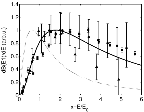
Figure 2: Comparison of scaled, experimental strength functions for $\@@nuc{6}{He}$ and $\@@nuc{11}{Li}$. The experimental data are: (circles) $\@@nuc{6}{He}$ – Aumann et al. [14], (triangles) $\@@nuc{11}{Li}$ – Sackett et al. [26], (squares) $\@@nuc{11}{Li}$ – Shimoura et al. [27]. The dotted curve is the two–body strength function from Ref [10, 11]. The solid line is the three–body strength function from Eq. (15).

In Fig. 2 several experimentally measured strength functions for $\@@nuc{6}{He}$ and $\@@nuc{11}{Li}$ are compared in the described way. The spectra are plotted as functions of the parameter $x=E/E_{0}$. The similarity of these scaled strength functions is evident. Such plots may be useful for quick predictions of shapes of E1 strength functions for two–neutron halo nuclei or for checking hypotheses on their three–body structure. Shown in this figure is also the analytical strength function from a two–body calculation where a Yukawa WF has been used together with plane waves in the final state [10, 11]. The two–body model gives a peak at too low energy thus clearly indicating the importance of using a three–body approach.

Now let us obtain the E1 strength function of Eq. (2) in our model. The final states (12) which can be reached from the ground state (11) via the dipole excitation are those with $K=1$ and $K=3$. Other selection rules are $\Delta l_{x}=0$, $\Delta l_{y}=\pm 1$, and $\Delta L=0,\pm 1$. The HH entering the final states (12) that contribute to the result for $\@@nuc{6}{He}$ are listed in Eq. (24). The required ME are sums of products of hyperangular ME and hyperradial integrals. The hyperangular ME entering the calculation are listed in Eq. (26). The hyperradial integrals are of the form (14), they can be calculated analytically and expressed (see e.g. [20]) in terms of the hypergeometrical functions. When the model (10), (11) is adopted for the bound state, one obtains the following final expression for the E1 strength function:

$$\frac{\mathrm{d}B(\mathrm{E}1)}{\mathrm{d}E}=c^{2}DE^{3}\sum_{i,j=0}^{1}\frac{(-1)^{i+j}\left[\alpha_{1}F_{1}(y_{i})F_{1}(y_{j})+\alpha_{2}F_{2}(y_{i})F_{2}(y_{j})\right]}{\left[(E_{i}+E)(E_{j}+E)\right]^{11/4}}.$$ (15)

Here $E$ is the continuum energy, $E_{0,1}=(\hbar\kappa_{0,1})^{2}/(2m)$, where $\kappa_{0}$, $\kappa_{1}$ and $c$ are defined in Eq. (10). The constant $D$ is

$$D=\frac{3}{2}\left(\frac{\hbar^{2}}{2m}\right)^{3/2}\frac{(Z_{\mathrm{c}}e)^{2}}{(A-2)A},$$

and the constants $\alpha_{1}$ and $\alpha_{2}$ are

$$\alpha_{1}=\frac{1}{4}\left(\frac{315}{2^{10}}\right)^{2}\left(1+3w_{00}+4\sqrt{w_{00}w_{20}}\right),\qquad\alpha_{2}=\left(\frac{9009\sqrt{3}}{2^{17}}\right)^{2}\left(w_{20}+w_{21}\right).$$

The coefficients $w_{00}$, $w_{20}$, and $w_{21}$ entering here are the weights of various HH, see Eq. (11). The quantities $y_{0,1}$ are defined as $y_{i}=E/(E+E_{i})$, and, finally,

$$F_{1}(y)=F\left(\frac{11}{4},\frac{3}{4},4,y\right),\qquad F_{2}(y)=yF\left(\frac{15}{4},\frac{7}{4},6,y\right),$$ (16)

where $F(\alpha,\beta,\gamma,z)$ is the standard hypergeometrical function [20]. The functions (16) represent the contributions from final states with $K=1$ and $K=3$, respectively. When the hyperradial function (9) is used the result is obviously obtained from Eq. (15) by retaining only the term with $i=j=0$ and replacing $c^{2}$ with $2\kappa_{0}$. At $E\rightarrow 0$ the strength function (15) exhibits the typical $E^{3}$ three–body behavior at threshold. (In reality “dineutron” correlations may influence the spectrum in the threshold region which is beyond our present consideration.)

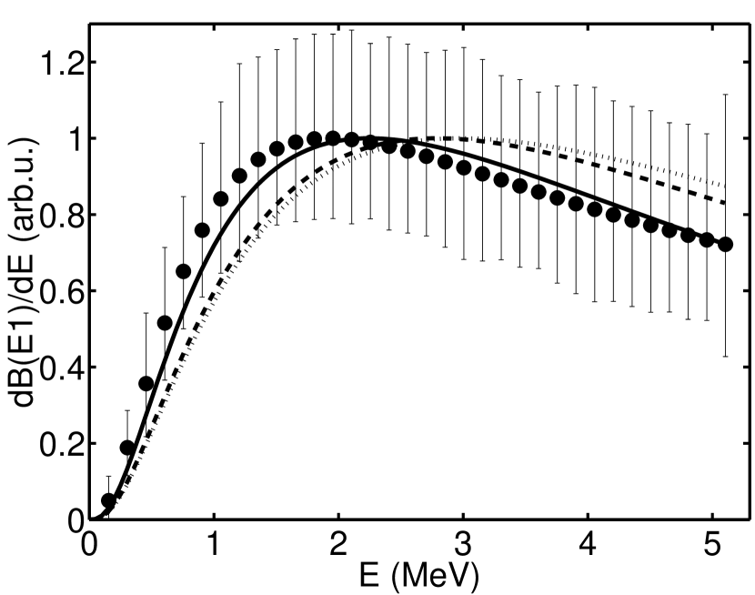
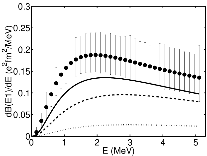
(a)

(b)

Figure 3: A comparison of our strength function with experimental data for $\@@nuc{6}{He}$, Aumann et al. [14], both in arbitrary units (a) and in absolute scale (b). The analytical strength functions are obtained with WFs $\Psi_{1}$ (dotted), $\Psi_{2}$ (dashed) and $\Psi_{3}$ (solid), see Table 1.

In Fig. 3 experimental data for the $\@@nuc{6}{He}$ strength function from Aumann et al. [14] (Pb target, $E_{\mathrm{lab}}=240$ MeV/nucleon) are compared to our model strength functions calculated with Eq. (15). The comparison is done both for the energy behavior of the spectra, Fig. 3(a), and in absolute scale, Fig. 3(b). From the comparison in Fig. 3(a) one sees that the shape of the spectrum is well reproduced by our model, especially in the case of the most complete version $\Psi_{3}$, see Table 1. A shift of the maximum to lower energies in the latter case is related to the inclusion of the contribution from the ground state HH with $K=0$. Maxima of the contributions from the HH with $K=2$ are shifted to higher energies since these HH lead in part to excitation of $K=3$ final states.

An interesting feature of the calculated strength functions seen in Fig. 3(a) is that when one passes from the hyperradial function (9) to the function (10) retaining the same hyperangular dependence (e.g. going from $\Psi_{1}$ to $\Psi_{2}$) the shape of the spectrum changes very little. This is explained by the above mentioned fact that only large $\rho$ values contribute sizably to the result. For such $\rho$ values only the first, longer range exponential in the hyperradial function (10) survives leading to just the same energy dependence as the model (9) (but to very different magnitudes of the cross section). Indeed, if one plots a figure similar to Fig. 1(b) but retaining only the contribution from the first exponential to the ME one obtains the integrands extremely close to those shown in Fig. 1(b). The same holds true for the $K=3$ final state. This means that the $i=j=0$ term dominates Eq. (15) at not too high energies. The other terms are suppressed by the factor $[(E_{0}+E)/(E_{1}+E)]^{11/4}$. At higher energies the model $\Psi_{2}$ leads to a strength function which decreases faster than that for the model $\Psi_{1}$. The internal part of the hyperradial function contributes more to the results here, and in the case of the two–parameter model this internal part is smaller than for the one–parameter model.

Comparing the magnitudes of the calculated strength functions with experiment in Fig. 3(b) one sees that the ground state model $\Psi_{1}$ (see Table 1) leads to a very low strength function. The results are considerably improved when passing to the model $\Psi_{2}$ while the model $\Psi_{3}$ leads to a further improvement and compares reasonably well with experiment. These results may be commented as follows. Underestimating the $\rho_{\mathrm{rms}}$ value the one–parameter model $\Psi_{1}$ underestimates simultaneously all sizes in the system including the distance $r_{\mathrm{c}}$ between the core and the CM, see Table 1. Furthermore, one needs to take into account that the E1 sum rule (5) strictly preserves its value if one replaces true final states with a complete set of no interaction final states. So, in our case the total strength is determined by the $r_{\mathrm{c}}$ value, and thus it is natural that the above model leads to a too low total strength. While the two–parameter WF, $\Psi_{2}$, reproduces correctly the rms matter radius it still gives an $r_{\mathrm{c}}$ value which is somewhat low. For this WF, which includes only one HH with $l_{x}=l_{y}$, we have the simple relation $\langle x^{2}\rangle=\langle y^{2}\rangle=\langle\rho^{2}\rangle/2$. However, this relation breaks down, due to off–diagonal terms in the expectation values, when more HH are included, as in $\Psi_{3}$, and the geometric properties of the state change slightly leading to a higher $r_{\mathrm{c}}$ value.

In accordance with the above discussion, at not too high energy the main effect of passing from the one–parameter model (9) to the two–parameter model (10) consists merely in the multiplication of the strength function by $c^{2}/(2\kappa_{0})\simeq 4$ which can be seen from comparing the strength functions for models $\Psi_{1}$ and $\Psi_{2}$ in Fig. 3(b). This is in principle similar to the case of photodisintegration of deutrons [21]. The cross section, calculated with the zero–range Yukawa ground state wave function $(2\kappa_{0})^{1/2}\exp(-\kappa r)/r$ and the no interaction final state, is lower than the experimental one. The main effect of the finite range correction consists in an increase of the asymptotic constant in the ground state WF leading to a reasonably good comparison with experiment at moderate energy.

In Table 2 the integrated strengths obtained are listed along with the experimental strengths and those obtained from a microscopic three–cluster calculation. The strengths are integrated up to $E=4$ MeV, $9$ MeV, and infinity. Note that for the first of these energies the ratio of the result obtained with $\Psi_{2}$ to that obtained with $\Psi_{1}$ is about $c^{2}/(2\kappa_{0})$ as it should be. Our total strength proved to be very close to that obtained using the microscopic bound state WF. These results on the total strength provide us also with a check of the strength function calculation. Integrating the strength function up to infinite energy one should reproduce the value of the sum rule (5).

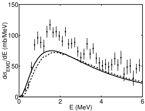
Figure 4: The $\@@nuc{6}{He}$ EMD excitation energy spectrum obtained at 240 MeV/A with a lead target. The data points are extracted from Ref. [14] while the solid line is our result obtained by multiplying the strength function (15) calculated for the $\Psi_{3}$ model with the spectrum of virtual photons. The dashed line is the same curve corrected for the LAND detector response and efficiency.

Finally, we calculate the EMD excitation energy spectrum using Eq. (1). The virtual photon spectrum was obtained for a $\@@nuc{6}{He}$ beam with energy 240 MeV/A striking a Pb target. In Fig. 4 the resulting distribution is compared with the excitation energy spectrum measured by Aumann et al. [14]. In Table 3 the total $\@@nuc{6}{He}$ cross sections obtained with our model are compared with experimental estimates for two different beam energies, 37 MeV/A and 240 MeV/A, measured at NSCL [22] and GSI [14] respectively. The theoretical cross section has been calculated by integrating the spectrum up to the energy $E=10$ MeV, corresponding approximately to the maximum energy measured in the experiments. The observed difference should be a direct measure of the importance of FSI since the virtual photon spectrum peaks at low energies and this is the region were FSI is supposed to play a role. We find that our model gives $\sim 35\%$ lower cross section than experiment for both energies.

4 Conclusion

A three–body model describing EMD of two–neutron halo nuclei, which allows studying the E1 strength functions without precise knowledge about initial and final states, has been developed. The model leads to an analytical expression for the strength functions. Our ground state wave functions reproduce both the true three–body asymptotics (determined by the binding energy) and the correct size of the system. A complete set of three–particle no interaction final states is used. We found that the large distance asymptotics of the ground state determines the shape of the strength function, while the size of the ground state governs the asymptotic constant and thus the magnitude of the strength function. We pointed out that in some cases the shapes of the E1 strength functions for different two–neutron halo nuclei are approximately related to each other.

We have used $\@@nuc{6}{He}$ as a test case and made an extensive comparison with experimental data [14, 22]. We found a good agreement concerning the shape and peak position of the E1 strength function and a reasonable agreement concerning its magnitude.

A remarkable feature of halo nuclei is that the E1 strength is concentrated at low energies even without any low–lying resonant state. This peculiarity is due to the low binding energy and large size of the initial state which is demonstrated by the present calculation with no final state interaction included in the model.

In a forthcoming paper, see also [23], we shall apply the present approach to investigate the E1 strength functions of Borromean $\@@nuc{11}{Li}$ and $\@@nuc{14}{Be}$ nuclei. Common for these nuclei are large uncertainties concerning their microscopic structure. In the $\@@nuc{11}{Li}$ case the E1 strength function is not so well known experimentally as in the $\@@nuc{6}{He}$ case, and for $\@@nuc{14}{Be}$ the EMD process has been measured only very recently [24].

As to the FSI effects, we noted that the total E1 strength will not change when replacing a complete set of no interaction final states with such a set of true final states. Therefore the only effect of including FSI will be a redistrubution of the strength leading to a somewhat higher strength at low energy. Further studies on this point would be of interest.

Appendix A Appendix

A.1 Coordinate sets and hyperspherical harmonics

We need to perform the calculation in the CM subsystem. The adopted Jacobi coordinates are

$$\begin{split}\vec{x}&=\frac{1}{\sqrt{2}}(\vec{r}_{1}-\vec{r}_{2}),\\ \vec{y}&=\sqrt{\frac{2(A-2)}{A}}\left(\frac{\vec{r}_{1}+\vec{r}_{2}}{2}-\vec{r}_{\mathrm{c}}\right),\end{split}$$ (17)

where $\vec{r}_{1}$, $\vec{r}_{2}$, and $\vec{r}_{\mathrm{c}}$ are positions of the valence nucleons and the core. We use the related hyperspherical coordinates $\{\rho,\Omega_{5}\}$. The hyperradius $\rho$ determines the size of a three–body state:

$$\rho^{2}=x^{2}+y^{2}=(\vec{r}_{1}-\vec{R}_{\mathrm{cm}})^{2}+(\vec{r}_{2}-\vec{R}_{\mathrm{cm}})^{2}+(A-2)(\vec{r}_{\mathrm{c}}-\vec{R}_{\mathrm{cm}})^{2}.$$ (18)

The five angles $\{\Omega_{5}\}$ include usual angles $(\theta_{x},\phi_{x})$, $(\theta_{y},\phi_{y})$ parametrizing the unit vectors $\hat{\bf x}$, $\hat{\bf y}$ and the hyperangle $\theta$ defined by the equalities

$$x=\rho\sin\theta,\qquad y=\rho\cos\theta,$$ (19)

where $0\leq\theta\leq\pi/2$. The volume element $d\Omega_{5}$ entering (7) is

$$\d\Omega_{5}=\sin^{2}\theta\cos^{2}\theta\d\theta\d\hat{\bf x}\d\hat{\bf y}.$$ (20)

The HH have the explicit form

$$\Gamma_{KLM_{L}}^{l_{x}l_{y}}\left(\Omega_{5}\right)=\psi_{K}^{l_{x}l_{y}}(\theta)Y_{LM_{L}}^{l_{x}l_{y}}(\hat{\bf x},\hat{\bf y}),$$ (21)

where

$$Y_{LM_{L}}^{l_{x}l_{y}}(\hat{\bf x},\hat{\bf y})=\left[Y_{l_{x}}(\hat{\bf x})\otimes Y_{l_{y}}(\hat{\bf y})\right]_{LM_{L}},$$ (22)

and $Y_{lm}$ are spherical harmonics. In Eq. (21) the hyperangular functions are

$$\psi_{K}^{l_{x}l_{y}}(\theta)=N_{K}^{l_{x}l_{y}}\sin^{l_{x}}\theta\cos^{l_{y}}\theta P_{n}^{l_{x}+1/2,l_{y}+1/2}(\cos 2\theta),$$

where $P_{n}^{\alpha,\beta}(x)$ are the Jacobi polynomials (see, e.g., [20]), $n=(K-l_{x}-l_{y})/2$, and $N_{K}^{l_{x}l_{y}}$ are normalization constants,

$$N_{K}^{l_{x}l_{y}}=\sqrt{\frac{2(n!)(K+2)(n+l_{x}+l_{y}+1)!}{\Gamma(n+l_{x}+3/2)\Gamma(n+l_{y}+3/2)}}.$$

The HH (21) are orthonormalized using the volume element (20).

A.2 E1 transition matrix elements

The explicit expressions for the HH entering our ground state are the following (see (19), (22) for notation):

$$\begin{split}\Gamma_{000}^{00}(\Omega_{5})&=\frac{4}{\sqrt{\pi}}\>Y_{00}^{00}(\hat{\bf x},\hat{\bf y}),\\ \Gamma_{200}^{00}(\Omega_{5})&=\frac{8}{\sqrt{\pi}}\cos 2\theta\>Y_{00}^{00}(\hat{\bf x},\hat{\bf y}),\\ \Gamma_{21M_{L}}^{11}(\Omega_{5})&=\frac{8}{\sqrt{3\pi}}\sin 2\theta\>Y_{1M_{L}}^{11}(\hat{\bf x},\hat{\bf y}).\end{split}$$ (23)

The explicit expressions for the final state HH contributing to our strength function are the following:

$$\begin{split}\Gamma_{11M_{L}}^{01}(\Omega_{5})&=\frac{8}{\sqrt{2\pi}}\cos\theta\>Y_{1M_{L}}^{01}(\hat{\bf x},\hat{\bf y}),\\ \Gamma_{11M_{L}}^{10}(\Omega_{5})&=\frac{8}{\sqrt{2\pi}}\sin\theta\>Y_{1M_{L}}^{10}(\hat{\bf x},\hat{\bf y}),\\ \Gamma_{31M_{L}}^{01}(\Omega_{5})&=-\frac{8}{\sqrt{6\pi}}(4\cos 2\theta+1)\cos\theta\>Y_{1M_{L}}^{01}(\hat{\bf x},\hat{\bf y}),\\ \Gamma_{31M_{L}}^{10}(\Omega_{5})&=\frac{8}{\sqrt{6\pi}}(4\cos 2\theta+1)\sin\theta\>Y_{1M_{L}}^{10}(\hat{\bf x},\hat{\bf y}),\\ \Gamma_{3LM_{L}}^{12}(\Omega_{5})&=\frac{32}{\sqrt{6\pi}}\cos^{2}\theta\sin\theta\>Y_{LM_{L}}^{12}(\hat{\bf x},\hat{\bf y}),\qquad L=1\,\,\mathrm{and}\,\,2.\end{split}$$ (24)

The E1 operator, Eq (4), can be written as

$$\mathcal{M}(\mathrm{E}1,\mu)=-eZ_{\mathrm{c}}\sqrt{\frac{2}{A(A-2)}}\rho\cos\theta Y_{1\mu}(\hat{\bf y}).$$

The ME

$$\langle K_{f}\,l_{x}\,l_{yf}\,L_{f}\,S,\,J_{f}=1,\,M_{f}=\mu|\cos\theta Y_{1\mu}(\hat{\bf y})|K_{i}\,l_{x}\,l_{yi}\,L_{i}\,S,\,J_{i}=0\rangle$$ (25)

of the hyperangular part of this operator, between basis states of the form

$$\left[\Gamma_{KL}^{l_{x}l_{y}}\left(\Omega_{5}\right)\otimes\theta_{S}\right]_{JM}$$

that include the HH (23) and (24) are required. We denote these ME as

$$\langle K_{f}\,l_{x}\,l_{yf}\,L_{f}\,S|O|K_{i}\,l_{x}\,l_{yi}\,L_{i}\,S\rangle.$$

The non–zero ME are

$$\begin{split}\langle 10110|O|00000\rangle=\frac{1}{2\sqrt{2\pi}},\qquad&\langle 10110|O|20000\rangle=\frac{1}{4\sqrt{2\pi}},\\ \langle 30110|O|20000\rangle=\frac{\sqrt{3}}{4\sqrt{2\pi}},\qquad&\langle 11011|O|21111\rangle=\frac{1}{4\sqrt{2\pi}},\\ \langle 31011|O|21111\rangle=\frac{1}{4\sqrt{6\pi}},\qquad&\langle 31211|O|21111\rangle=\frac{1}{4\sqrt{3\pi}},\\ \langle 31221|O|21111\rangle=\frac{1}{4\sqrt{\pi}}.\qquad&\end{split}$$ (26)

The calculation with respect to spin variables and angles $\hat{\bf x}$, $\hat{\bf y}$ is done using the formula (see, e.g., [25]) expressing the ME (25) in terms of reduced ME in the $\hat{\bf x},\hat{\bf y}$ subspace and then in terms of reduced ME in the $\hat{\bf y}$ subspace. Finally, note that the results obtained in this section are useful not only for $\@@nuc{6}{He}$ but also when studying other two–neutron halo nuclei.

Table 1: The model WFs for $\@@nuc{6}{He}$. The parameter $\kappa_{0}$ reproduces the two–neutron separation energy. The last three columns give the hyperradius $\rho_{\mathrm{rms}}$, the matter radius $R_{\mathrm{rms}}$ and the distance between the core and the CM $r_{\mathrm{c}}$.

WF	$\kappa_{0}$	$\kappa_{1}$	$w_{00}$	$w_{20}$	$w_{21}$	$\rho_{\mathrm{rms}}$	$R_{\mathrm{rms}}$	$r_{\mathrm{c}}$
	(fm-1)	(fm-1)				(fm)	(fm)	(fm)
$\Psi_{1}$	0.2163	—	0	1	0	3.27	1.79	0.67
$\Psi_{2}$	0.2163	0.5370	0	1	0	5.37	2.50	1.10
$\Psi_{3}$	0.2163	0.5370	0.05	0.80	0.15	5.37	2.50	1.20

Table 2: The $\@@nuc{6}{He}$ integrated strength $\int_{0}^{E}\d E^{\prime}\;\d B(\mathrm{E}1)/\d E^{\prime}$, where $E$ is the continuum energy, for different models and experimental data. The last column corresponds to $E=\infty$ and equals to the result of Eq. (5). All values are given in $e^{2}\mathrm{fm}^{2}$.

	$E=4$ MeV		$E=9$ MeV		Total B(E1)
Aumann et al [14]	0.	59(12)	1.	2(2)
$\Psi_{1}$	0.	079	0.	18	0.43
$\Psi_{2}$	0.	29	0.	63	1.14
$\Psi_{3}$	0.	42	0.	83	1.38
Realistic WF	0.	71	1.	02	1.37

Table 3: The $\@@nuc{6}{He}$ EMD cross section obtained with a lead target at different energies. The theoretical values are obtained by integrating (1) up to 10 MeV.

Energy (MeV/A)	Exp.		This work
	$\sigma_{\mathrm{EMD}}$ (mb)	Ref.	$\sigma_{\mathrm{EMD}}$ (mb)
37	830	[22]	551
240	$520\pm 110$	[14]	333

References

- [1] P. G. Hansen and B. Jonson, Euro. Lett. 4, 409 (1987).
- [2] T. Kobayashi et al., Phys. Lett. B 232, 51 (1989).
- [3] Y. Suzuki, Nucl. Phys. A 528, 395 (1991).
- [4] H. Esbensen and G. F. Bertsch, Nucl. Phys. A 542, 310 (1992).
- [5] K. Ikeda, Nucl. Phys. A 538, 355c (1992).
- [6] B. V. Danilin, M. V. Zhukov, J. S. Vaagen, and J. M. Bang, Phys. Lett. B 302, 129 (1993).
- [7] A. Csótó, Phys. Rev. C 49, 3035 (1994).
- [8] S. Funada, H. Kameyama, and Y. Sakuragi, Nucl. Phys. A 575, 93 (1994).
- [9] B. V. Danilin, I. J. Thompson, J. S. Vaagen, and M. V. Zhukov, Nucl. Phys. A 632, 383 (1998).
- [10] C. A. Bertulani and G. Baur, Nucl. Phys. A 480, 615 (1988).
- [11] T. Otsuka, M. Ishihara, N. Fukunishi, T. Nakamura, and M. Yokoyama, Phys. Rev. C 49, R2289 (1994).
- [12] A. Cobis, D. V. Fedorov, and A. S. Jensen, Phys. Rev. C 58, 1403 (1998).
- [13] A. Pushkin, B. Jonson, and M. V. Zhukov, J. Phys. G 22, 95 (1996).
- [14] T. Aumann et al., Phys. Rev. C 59, 1252 (1999).
- [15] A. Winther and K. Alder, Nucl. Phys. A 319, 518 (1979).
- [16] C. A. Bertulani and G. Baur, Nucl. Phys. A 442, 739 (1985).
- [17] M. V. Zhukov et al., Phys. Rep. 231, 151 (1993).
- [18] S. P. Merkuriev, Sov. J. Nucl. Phys. 19, 222 (1974).
- [19] C. Forssén, B. Jonson, and M. V. Zhukov, Nucl. Phys. A 673, 143 (2000).
- [20] I. S. Gradshteyn and I. M. Ryzhik, Table of Integrals, Series and Products, Academic Press, Inc., San Diego, second edition, 1980.
- [21] J. S. Levinger, Nuclear photo–disintegration, Oxford University Press, London, 1960.
- [22] R. E. Warner et al., Phys. Rev. C 62, 024608(9) (2000).
- [23] C. Forssén, Borromean halo nuclei – an analytical study of breakup reactions, Chalmers University of Technology and Göteborg University, 2000, Licenciate Thesis.
- [24] M. Labiche et al., Phys. Rev. Lett. 86, 600 (2001).
- [25] D. A. Varshalovich, A. N. Moskalev, and V. K. Khersonskii, Quantum Theory of Angular Momentum, World Scientific, Singapore, 1989.
- [26] D. Sackett et al., Phys. Rev. C 48, 118 (1993).
- [27] S. Shimoura et al., Phys. Lett. B 348, 29 (1995).
- [28] G. F. Bertsch, K. Hencken, and H. Esbensen, Phys. Rev. C 57, 1366 (1998).
(a)
(b)
(a)
(b)