In medium $T$-matrix for superfluid nuclear matter

Abstract

We study a generalized ladder resummation in the superfluid phase of the nuclear matter. The approach is based on a conserving generalization of the usual $T$-matrix approximation including also anomalous self-energies and propagators. The approximation here discussed is a generalization of the usual mean-field BCS approach and of the in medium $T$-matrix approximation in the normal phase. The numerical results in this work are obtained in the quasi-particle approximation. Properties of the resulting self-energy, superfluid gap and spectral functions are studied.

21.65+f, 24.10Cn, 26.60+c

1 Introduction

One of the most general properties of fermion systems with attractive interactions is the transition to a superfluid state at finite density and low temperature. It is expected that such a phenomenom happens also for the strongly interacting system of nucleons, i.e for cold nuclear matter. Calculations based on nucleon-nucleon interaction predict very large values of the superfluid gap. Typically around $5-10$MeV for the isospin singlet ($T=0$) partial-wave ${}^{3}S_{1}-^{3}D_{1}$ [1, 2, 3, 4]. The actual value of the superfluid gap is a matter of debate, because of expected screening and self-energy corrections. One has to note that also some of the phenomenological potentials fitted to the pairing properties of finite nuclei give significant values of the superfluid gap in nuclear matter [5]. The study of $T=0$ pairing in the systematics of $N\simeq Z$ nuclei became possible with advent of radioactive beam facilities. This lead to a resurgence of the study of the nuclear mass systematics [6, 7, 8]. Thus it is of importance to obtain results on the nature of the nuclear pairing ($T=0$ or $T=1$) and the value of the superfluid gap for symmetric nuclear matter at saturation density and below. It appears that the mean-field gap equation without medium modifications is unrealistic [9, 10, 11, 12, 13, 14] and hence the best strategy would be to calculate a density dependent gap for nuclear matter (including relevant many-body corrections) and use it in a local density approximation for calculations in finite systems [5, 7].

The neutron rich nuclear matter is used in modeling of the crust and of the core of neutron stars. It is generally believed that such an asymmetric nuclear matter is superfluid, with different kinds of superfluid gap appearing in the vast range of densities present in the neutron star. The value of the superfluid gap is of importance for fundamental problems in the neutron stars, the formation of glitches, the value of the viscosity and the cooling rates in different scenarios [15]. Again one of the possible approaches is to calculate the superfluid gap from bare $NN$ interaction using the Brueckner-Hartree-Fock approximation to get single-particle energies for the gap equation [16, 17, 11, 18, 19, 13, 14, 20]. However, in order to obtain reliable estimates for the superfluid gap in the neutron matter we need to have under control in medium many-body corrections to the gap equation.

As noted above strong modifications of the mean-field result for the superfluid gap are expected in the nuclear matter due to screening effects [9, 10, 11], modifications of the effective mass and self-energy corrections [12, 14, 13]. One of the motivations of the present study is to investigate another source of in medium correction to the value of the gap. These corrections occur in a generalization of the resummation of ladder diagrams to include also anomalous propagators. In the following we study the formalism and give numerical estimates of the corrections to the anomalous self-energy. These additional terms introduce an energy dependence in the superfluid gap, but the modifications of the value of the gap at the Fermi surface are not as dramatic as from the other medium effects.

The correction to the binding energy due to the superfluid rearrangement of the ground state is believed to be small [21]. However, some of the calculations using realistic nuclear forces predict quite large values of the superfluid gap in the nuclear matter. A large superfluid gap could lead to modifications of the normal part of the self-energy and the spectral function. In the following we study a consistent approximation treating on equal footing the normal and anomalous part of the self-energy. We find that important modifications of the single-particle and two-body propagators appear if the superfluid gap is large. These significant modifications in the superfluid present, a posteriori, an important reason to consider the generalized formalism discussed in this work. Also the expansion of the ground state energy or other quantities around the wrong ground state is not satisfactory for a theory aiming at the description of the many-body problem from first-principles, using free nucleon-nucleon potentials. The incorrect ground state could also lead to instabilities in the actual iterative numerical solution of the many-body equations, related to the appearance of the Cooper instability [22].

Mean-field approaches give a qualitatively correct description of the formation of the superfluid gap by the BCS mechanism, but fail in the resummation of the hard core. Recently superfluid nuclear matter was studied in an approach starting from the in medium $T$-matrix approximation [23]. The resummation of ladder diagrams in the $T$-matrix can be used to deal with the hard core in the interaction potential. The $T$-matrix approximation for the self-energy was studied intensively in the last decade in normal nuclear matter. It is different from the usual $G$-matrix approximation. The $T$-matrix formalism, also called self-consistent Green’s function approach, can be used directly at high temperature, above the superfluid phase transition[24, 25, 26, 27]. It allows to study in a self-consistent way the one-particle self-energies and spectral functions [24, 26, 28, 29, 30], the two-particle properties and in medium cross-sections [24, 25, 26, 27, 31, 29], the onset of superfluidity [32, 33, 20, 23, 29], the self-energy corrections to the superfluid gap [12]. The treatment of the old question of saturation properties of nuclear matter in the $T$-matrix approximation is at the present stage not superior to the most recent $G$ matrix or variational calculations, including realistic interactions, three-body and three-body forces corrections. However, the $T$-matrix self-energy leads to reliable results for the single particle properties, in particular it gives a consistent value for the Fermi energy fulfilling the Hugenholz-Van Hove theorem [34, 27].

Besides the above motivations to develop the $T$-matrix approach for nuclear matter, this approximation seems to be the most natural starting point for the study of the superfluid phase of the nuclear matter. The appearance of a singularity in the $T$-matrix at zero total momentum of the pair and at twice the Fermi energy signals the formation of a long range order and defines the Thouless criterion for the critical temperature. It is in fact equivalent to the critical temperature corresponding to the appearance of a nontrivial solution of the BCS gap equation. The same is true if off-shell propagators are used in the $T$-matrix ladders. It corresponds to a generalization of the gap equation to one using full spectral functions, including the imaginary part of the normal self-energy [12]. The study of the singularity in the $T$-matrix equations at finite temperature, in the normal phase, allows to identify the critical temperature and the precritical modifications of the spectral function, in medium cross-sections and density of states [32, 33, 20, 35, 29, 26, 23, 36].

The generalization of the $T$-matrix approximation to the superfluid phase appearing below $T_{c}$ was discussed in Ref [23]. The approach is based on the observation that the formation of the superfluid order parameter requires a long range order. This long range order, representing the formation of Cooper pairs at zero momentum and twice the Fermi energy, corresponds to a singularity in the $T$-matrix for the same energy and momentum as in the Thouless criterion. Thus also below $T_{c}$ we expect the singularity in the two-body propagator at twice the Fermi energy. The kernel of the $T$-matrix equation is modified in the superfluid so that the singularity of the $T$-matrix equation is again equivalent to the BCS gap equation for non-zero values of the order parameter [23].

In the present work we investigate a different approach to the $T$-matrix resummation in the superfluid. It is a generalization of the ordinary $T$-matrix ladder diagrams which includes also anomalous propagators. Thus normal and anomalous self-energies are calculated in a unified way. The approximation deals at the same time with ladder diagrams resummation for the self-energy and with the appearance of the order parameter. The properties of the generalized $T$-matrix, self-energy and spectral function are discussed. A justification of the heuristic procedure of Ref. [23] is then obtained if the superfluid order parameter is restricted to the BCS contribution. The practical calculations are more difficult in the generalized scheme here discussed. The number of propagators and $T$-matrix components is doubled because of the appearance of the off-diagonal, anomalous propagators. The numerical results presented in this work are obtained in the quasi-particle approximation, starting from mean-field BCS propagators.

2 Green’s functions in the superfluid

2.1 Notation and formulas for the normal phase

We consider infinite homogenous nuclear matter interacting through a two-body potential. The energies are defined with respect to the chemical potential $\mu$

$$H=\sum_{\alpha}\int d^{3}x\ \Psi_{\alpha}^{\dagger}(x)(-\frac{\Delta}{2m}-\mu)\Psi_{\alpha}(x)$$

$$+\sum_{\alpha^{{}^{\prime}},\beta^{{}^{\prime}},\alpha,\beta}\frac{1}{2}\int d^{3}x\int d^{3}y\Psi_{\alpha^{{}^{\prime}}}^{\dagger}(x)\Psi_{\beta^{{}^{\prime}}}^{\dagger}(y)V_{\alpha^{{}^{\prime}},\beta^{{}^{\prime}},\alpha,\beta}(x,y)\Psi_{\beta}(y)\Psi_{\alpha}(x)\ .$$ (1)

In the real time formalism the Green’s functions are defined on a contour in the time plane [37]. It means that as functions of a single valued time variable the Green’s functions acquire a matrix structure

$${\hat{G}_{\alpha\beta}(x_{1},t_{1};x_{2},t_{2})}=\left(\matrix{G_{\alpha\beta}^{c}(x_{1},t_{1};x_{2},t_{2})&G_{\alpha\beta}^{<}(x_{1},t_{1};x_{2},t_{2})\cr G_{\alpha\beta}^{>}(x_{1},t_{1};x_{2},t_{2})&G_{\alpha\beta}^{a}(x_{1},t_{1};x_{2},t_{2})}\right)\ \ \ .$$ (2)

Where $G_{\alpha\beta}^{c}(x_{1},t_{1};x_{2},t_{2})=i\langle T\Psi_{\alpha}(x_{1},t_{1})\Psi_{\beta}^{\dagger}(x_{2},t_{2})\rangle$ is the chronological Green’s function, $G^{a}$ is the anti-chronological Green’s function and $G_{\alpha\beta}^{<}(x_{1},t_{1};x_{2},t_{2})=i\langle\Psi_{\alpha}(x_{1},t_{1})\Psi_{\beta}^{\dagger}(x_{2},t_{2})\rangle$ and $G_{\alpha\beta}^{<}(x_{1},t_{1};x_{2},t_{2})=-i\langle\Psi_{\beta}^{\dagger}(x_{2},t_{2})\Psi_{\alpha}(x_{1},t_{1})\rangle$ are the correlation functions. In a homogeneous system, after Fourier transforming in the relative coordinate and time, single-particle Green’s functions depend on a single energy and momentum. Noting that the Green’s function are diagonal in the spin-isospin indices, we can write

$$\hat{G}_{\alpha\beta}(p,\omega)=\delta_{\alpha\beta}\hat{G}(p,\omega)\ .$$ (3)

A single scalar function (in spin-isospin indices) $G$ is sufficient to describe a spin and isospin symmetric nuclear matter. The scalar correlation functions are written using the spectral function

$$G^{<}(p,\omega)=if(\omega)A(p,\omega)$$ (4)

$$G^{>}(p,\omega)=-i(1-f(\omega))A(p,\omega)\ \ .$$ (5)

$f(\omega)=\frac{1}{1+\exp{-\beta(\omega-\mu)}}$ is the Fermi distribution at temperature $T=1/\beta$. The spectral function $A$ can be related to the retarded Green’s function

$$A(p,\omega) = -2{\rm Im}G^{+}(p,\omega)$$ (6)

$$= i\big{(}G^{>}(p,\omega)-G^{<}(p,\omega)\big{)}$$

$$= \frac{-2{\rm Im}\Sigma^{+}(p,\omega)}{(\omega-p^{2}/2m-{\rm Re}\Sigma^{+}(p,\omega)+\mu)^{2}+{\rm Im}\Sigma^{+}(p,\omega)^{2}}\ ,$$ (7)

where $\Sigma^{+}(p,\omega)$ is the retarded self-energy.

The $T$-matrix equation in the normal phase is

$$\langle{\bf p}|T_{\alpha^{{}^{\prime}}\beta^{{}^{\prime}}\alpha\beta}^{\pm}({\bf P},\omega)|{\bf p}^{{}^{\prime}}\rangle = V_{\alpha^{{}^{\prime}}\beta^{{}^{\prime}}\alpha\beta}({\bf p},{\bf p}^{{}^{\prime}})$$ (8)

$$+\sum_{\gamma\delta}\int\frac{d^{3}k}{(2\pi)^{3}}\int\frac{d^{3}q}{(2\pi)^{3}}V_{\alpha^{{}^{\prime}}\beta^{{}^{\prime}}\gamma\delta}({\bf p},{\bf k})$$

$$\langle{\bf k}|{\cal G}^{\pm}({\bf P},\omega)|{\bf q}\rangle\langle{\bf q}|T_{\gamma\delta\alpha\beta}^{\pm}({\bf P},\omega)|{\bf p}^{{}^{\prime}}\rangle\ ,$$

where ${\cal G}$ is the disconnected retarded two-particle propagator

$$\langle{\bf p}|{\cal G}^{\pm}({\bf P},\omega)|{\bf p}^{{}^{\prime}}\rangle=(2\pi)^{3}\delta^{3}({\bf p}-{\bf p}^{{}^{\prime}})\int\frac{d\omega^{{}^{\prime}}}{2\pi}\int\frac{d\omega^{{}^{\prime\prime}}}{2\pi}$$

$$\Big{(}G^{<}({\bf P}/2+{\bf p},\omega^{{}^{\prime\prime}}-\omega^{{}^{\prime}})G^{<}({\bf P}/2-{\bf p},\omega^{{}^{\prime}})$$

$$-G^{>}({\bf P}/2+{\bf p},\omega^{{}^{\prime\prime}}-\omega^{{}^{\prime}})G^{>}({\bf P}/2-{\bf p},\omega^{{}^{\prime}})\Big{)}/\Big{(}\omega-\omega^{{}^{\prime\prime}}\pm i\epsilon\Big{)}$$

$$=(2\pi)^{3}\delta^{3}({\bf p}-{\bf p^{{}^{\prime}}}){\cal G}^{\pm}({\bf P},\omega,{\bf p})\ .$$ (9)

Note that it is sufficient to solve a single equation for the retarded $T$-matrix instead of a matrix equation in the indices on the time contour in the complex time plane (2).

A full structure in the spin-isospin indices and relative angles of momenta must be kept. However, usually a partial wave expansion of the $T$-matrix equation is performed

$$\langle{p}|T^{(JST)\ \pm}_{l^{{}^{\prime}}l}({P},\omega)|{p}^{{}^{\prime}}\rangle = V^{(JST)}_{l^{{}^{\prime}}l}({p},{p}^{{}^{\prime}})+\sum_{l^{{}^{\prime\prime}}}\int\frac{k^{2}dk}{2\pi^{2}}V_{l^{{}^{\prime}}l^{{}^{\prime\prime}}}^{(JST)}({p},{k})$$ (10)

$${\cal G}^{\pm}({P},\omega,k)\langle{k}|T^{(JST)\ \pm}_{l^{{}^{\prime\prime}}l}({P},\omega)|{p}^{{}^{\prime}}\rangle\$$

after angle averaging the Kernel ${\cal G}$

$${\cal G}^{\pm}(P,\omega,p)=\int\frac{d\Omega}{4\pi}{\cal G}^{\pm}({\bf P},\omega,{\bf p})\ .$$ (11)

2.2 Anomalous Green’s function

In the superfluid phase the ground state of the system has a nonzero order parameter, corresponding to bound Cooper pairs [38]. This leads to new Green’s functions

$${\hat{F}_{\alpha\beta}(x_{1},t_{1};x_{2},t_{2})}=\left(\matrix{F_{\alpha\beta}^{c}(x_{1},t_{1};x_{2},t_{2})&F_{\alpha\beta}^{<}(x_{1},t_{1};x_{2},t_{2})\cr F_{\alpha\beta}^{>}(x_{1},t_{1};x_{2},t_{2})&F_{\alpha\beta}^{a}(x_{1},t_{1};x_{2},t_{2})}\right)\ \ \ .$$ (12)

$F^{c}$ is the time ordered anomalous Green’s function

$$F_{\alpha\beta}^{c}(x_{1},t_{1};,x_{2},t_{2})=i\langle T(\Psi_{\alpha}(x_{1},t_{1})\Psi_{\beta}(x_{2},t_{2}))\rangle$$

and $F^{a}$ the anti-chronological one and where

$$F_{\alpha\beta}^{<}(x_{1},t_{1};,x_{2},t_{2}) = i\langle\Psi_{\alpha}(x_{1},t_{1})\Psi_{\beta}(x_{2},t_{2})\rangle\noindent$$ (13)

$$F_{\alpha\beta}^{>}(x_{1},t_{1};,x_{2},t_{2}) = -i\langle\Psi_{\beta}(x_{2},t_{2})\Psi_{\alpha}(x_{1},t_{1})\rangle\ \ .$$ (14)

We consider a homogeneous infinite system so that the anomalous Green’s functions depend on a single momentum and energy. Analogously as for the normal Green’s functions we can write

$$F_{\alpha\beta}^{<}(p,\omega) = if(\omega)B_{\alpha\beta}(p,\omega)\noindent$$ (15)

$$F_{\alpha\beta}^{>}(p,\omega) = -i(1-f(\omega))B_{\alpha\beta}(p,\omega)\ \ .$$ (16)

The anomalous spectral function is related to the imaginary part of the retarded propagator

$$B_{\alpha\beta}(p,\omega) = -{\rm Im}\big{(}F^{+}_{\alpha\beta}(p,\omega+i\epsilon\big{)}-F^{+}_{\alpha\beta}(p,\omega-i\epsilon))\noindent$$ (17)

$$= i\big{(}F^{>}_{\alpha\beta}(p,\omega)-F^{<}_{\alpha\beta}(p,\omega)\big{)}$$ (18)

It should be noted that the spectral function for the diagonal part of the Green’s function is modified in the presence of the off-diagonal self-energy $\Delta$. We shall denote it by

$$A_{s}(p,\omega)=-2{\rm Im}G^{+}(p,\omega)$$ (19)

and reserve the notation $A(p,\omega)$ to the spectral function obtained by putting $\Delta=0$ (Eq. 7).

The spin-isospin structure of the anomalous Green’s function is assumed to be of the spin (isospin) singlet or triplet kind. We write

$$F_{\alpha\beta}(p,\omega)=\tilde{\Delta}_{\alpha\beta}F(p,\omega)\ \ .$$ (20)

In general the matrix $\tilde{\Delta}_{\alpha\beta}$ could depend on the momentum, energy and relative directions of spin, isospin and momentum. To simplify we use in the following angle-averaged double propagators in the $T$-matrix ladder. The matrix $\tilde{\Delta}$ in spin-isospin fulfills

$$\tilde{\Delta}^{\dagger}_{\alpha\beta}\tilde{\Delta}_{\beta\gamma}=|D|^{2}\delta_{\alpha\gamma}$$ (21)

for time-reversal invariant states. Without loss of generality we can put $|D|^{2}=1$. More specifically the spin (isospin) part of $\tilde{\Delta}_{\alpha\beta}$ is

$$\left(\matrix{d_{x}+id_{y}&-id_{z}\cr-id_{z}&d_{x}-id_{y}}\right)$$ (22)

for the triplet gap ($d_{x}^{2}+d_{y}^{2}+d_{z}^{2}=1$) and

$$\left(\matrix{0&i\cr-i&0}\right)$$ (23)

for the singlet one. Together with the choice of a diagonal normal Green’s function we describe the propagators using scalar functions in spin-isospin indices $F^{<>}(p,\omega)$ and $G^{<>}(p,\omega)$ or the corresponding retarded propagators and spectral functions.

2.3 Ladder resummation in the superfluid

Ladder resummations in the superfluid have been considered in the description of high $T_{c}$ superconductors [39]. A thermodynamically consistent scheme which reduces to the usuall $T$-matrix equation above $T_{c}$ can be constructed. The simplest way is to introduce a generalised $T$-matrix with aditional indices indicating if the incoming line is anomaleous or normal, following the Nambu formalism for superconductors. Rescticting oneself to two normal or two anomalous propagators in the ladder leads to the following additional matrix structure in the $T$-matrix

$$\left(\matrix{\langle{\bf p}|T^{\pm}_{\alpha^{{}^{\prime}}\beta^{{}^{\prime}}\alpha\beta}({\bf P},\Omega)|{\bf p^{{}^{\prime}}}\rangle&\langle{\bf p}|L^{\pm}_{\alpha^{{}^{\prime}}\beta^{{}^{\prime}}\alpha\beta}({\bf P},\Omega)|{\bf p^{{}^{\prime}}}\rangle\cr\langle{\bf p}|L^{\pm\ \dagger}_{\alpha^{{}^{\prime}}\beta^{{}^{\prime}}\alpha\beta}({\bf P},-\Omega)|{\bf p^{{}^{\prime}}}\rangle&\langle{\bf p}|T^{\pm\dagger}_{\alpha^{{}^{\prime}}\beta^{{}^{\prime}}\alpha\beta}({\bf P},-\Omega)|{\bf p^{{}^{\prime}}}\rangle}\right)=$$

$$\left(\matrix{V({\bf p},{\bf p^{{}^{\prime}}})_{\alpha^{{}^{\prime}}\beta^{{}^{\prime}}\alpha\beta}&0\cr 0&V({\bf p},{\bf p^{{}^{\prime}}})_{\alpha^{{}^{\prime}}\beta^{{}^{\prime}}\alpha\beta}}\right)+\int\frac{d^{3}q}{(2\pi)^{3}}\sum_{\gamma\delta}\left(\matrix{V({\bf p},{\bf q})_{\alpha^{{}^{\prime}}\beta^{{}^{\prime}}\gamma^{{}^{\prime}}\delta^{{}^{\prime}}}&0\cr 0&V({\bf p},{\bf q})_{\alpha^{{}^{\prime}}\beta^{{}^{\prime}}\gamma^{{}^{\prime}}\delta^{{}^{\prime}}}}\right)$$

$$\left(\matrix{\delta_{\gamma\gamma^{{}^{\prime}}}\delta_{\delta\delta^{{}^{\prime}}}{\cal G}^{\pm}({\bf P},\Omega,{\bf q})&{\cal H}^{\pm}_{\gamma\delta\gamma^{{}^{\prime}}\delta^{{}^{\prime}}}({\bf P},\Omega,{\bf q})\cr{\cal H}^{\pm\dagger}_{\gamma\delta\gamma^{{}^{\prime}}\delta^{{}^{\prime}}}({\bf P},-\Omega,{\bf q})&\delta_{\gamma\gamma^{{}^{\prime}}}\delta_{\delta\delta^{{}^{\prime}}}{\cal G}^{\pm}({\bf P},-\Omega,{\bf q})}\right)$$

$$\left(\matrix{\langle{\bf q}|T^{\pm}_{\gamma^{{}^{\prime}}\delta^{{}^{\prime}}\alpha\beta}({\bf P},\Omega)|{\bf p^{{}^{\prime}}}\rangle&\langle{\bf q}|L^{\pm}_{\gamma^{{}^{\prime}}\delta^{{}^{\prime}}\alpha\beta}({\bf P},\Omega)|{\bf p^{{}^{\prime}}}\rangle\cr\langle{\bf q}|L_{\gamma^{{}^{\prime}}\delta^{{}^{\prime}}\alpha\beta}^{\pm\ \dagger}({\bf P},-\Omega)|{\bf p^{{}^{\prime}}}\rangle&\langle{\bf q}|T^{\pm\dagger}_{\gamma^{{}^{\prime}}\delta^{{}^{\prime}}\alpha\beta}({\bf P},-\Omega)|{\bf p^{{}^{\prime}}}\rangle}\right)$$ (24)

where

$${\cal H}^{\pm}_{\gamma\delta\alpha\beta}({\bf P},\Omega,{\bf p})=\int\frac{d\omega^{{}^{\prime}}}{2\pi}\int\frac{d\omega^{{}^{\prime\prime}}}{2\pi}$$

$$\Big{(}F^{<}_{\alpha\gamma}({\bf P}/2+{\bf p},\omega^{{}^{\prime\prime}}-\omega^{{}^{\prime}})F^{<}_{\beta\delta}({\bf P}/2-{\bf p},\omega^{{}^{\prime}})$$

$$-F^{>}_{\alpha\gamma}({\bf P}/2+{\bf p},\omega^{{}^{\prime\prime}}-\omega^{{}^{\prime}})F^{>}_{\beta\delta}({\bf P}/2-{\bf p},\omega^{{}^{\prime}})\Big{)}/\Big{(}\Omega-\omega^{{}^{\prime\prime}}\pm i\epsilon\Big{)}\$$ (25)

denotes two disconnected anomalous propagators. $L^{\pm}$ is the off-diagonal part of the generalized retarded $T$-matrix (Fig. 1).

The anomalous part of the ladder ${\cal H}_{\alpha\beta\gamma\delta}$ does not mix different values of the total spin (isospin) of the pair. It can be seen by writing the matrix structure of $H_{\alpha\beta}$ in the basis of the total spin (isospin) of the pair and of its third component.

$${\cal H}=\left(\matrix{(d_{x}+d_{y})^{2}&-i\sqrt{2}d_{z}(d_{x}+id_{y})&-d_{z}^{2}&0\cr-i\sqrt{2}d_{x}(d_{x}+id_{y})&d_{x}^{2}+d_{y}^{2}-d_{z}^{2}&-i\sqrt{2}d_{z}(d_{x}-id_{y})&0\cr-d_{z}^{2}&-id_{z}(d_{x}-id_{y})&(d_{x}-id_{y})^{2}&0\cr 0&0&0&D^{2}}\right)H$$ (26)

for the triplet pairing with the matrix in the components $1^{+},1^{0},1^{-},0^{0}$ of the total spin (isospin) of the pair and

$${\cal H}=\left(\matrix{0&0&-1&0\cr 0&1&0&0\cr-1&0&0&0\cr 0&0&0&1}\right)H$$ (27)

for the singlet pairing. Using the structure of the anomalous Green’s function (Eq. 20) and assuming a dependence of the angle averaged spin-isospin structure (the matrices in Eqs. 26, 27) only on the value of total momentum one finds for central forces

$$\sum_{\gamma\delta}{\cal H}_{\alpha^{{}^{\prime}}\beta^{{}^{\prime}}\gamma\delta}\times{\cal H}_{\gamma\delta\alpha\beta}=\delta_{\alpha^{{}^{\prime}}\beta}\delta_{\alpha\beta^{{}^{\prime}}}{H}^{\dagger}\times{H}\ ,$$ (28)

where $\times$ stands for momentum integrals with the interaction potential or the $T-$matrix as occurring in the iteration of the Eq. (2.3). Thus partial wave decomposition can be applied after angular averaging of the intermediate uncorrelated two normal or two anomalous propagators in the ladder. The resulting generalized $T$-matrix equation has a matrix structure corresponding to (Eq. 2.3) in each partial wave

$$\left(\matrix{\langle{p}|T^{\pm}_{(JST)}({P},\Omega)|{p^{{}^{\prime}}}\rangle&\langle{p}|L^{\pm}_{(JST)}({P},\Omega)|{p^{{}^{\prime}}}\rangle\cr\langle{p}|L^{\pm}_{(JST)}({P},\Omega)|{p^{{}^{\prime}}}\rangle&\langle{p}|T^{\pm\dagger}_{(JST)}({P},-\Omega)|{p^{{}^{\prime}}}\rangle}\right)=$$

$$\left(\matrix{V_{(JST)}({p},{p^{{}^{\prime}}})&0\cr 0&V_{(JST)}({p},{p^{{}^{\prime}}})}\right)+\int\frac{q^{2}dq}{2\pi^{2}}\left(\matrix{V_{(JST)}({p},{q})&0\cr 0&V_{(JST)}({p},{q})}\right)$$

$$\left(\matrix{{\cal G}^{\pm}({P},\Omega,q)&{\cal H}^{\pm}({P},\Omega,q)\cr{\cal H}^{\pm\dagger}({P},-\Omega,q)&{\cal G}^{\pm}({P},-\Omega,q)}\right)$$

$$\left(\matrix{\langle{q}|T^{\pm}_{(JST)}({P},\Omega)|{p^{{}^{\prime}}}\rangle&\langle{q}|L^{\pm}_{(JST)}({P},\Omega)|{p^{{}^{\prime}}}\rangle\cr\langle{q}|L^{\pm}_{(JST)}({P},\Omega)|{p^{{}^{\prime}}}\rangle&\langle{q}|T^{\pm\dagger}_{(JST)}({P},-\Omega)|{p^{{}^{\prime}}}\rangle}\right)\ .$$ (29)

We used also $\langle p|L^{\pm}(P,\Omega)|q\rangle=\langle p|L^{\pm\ \dagger}(P,-\Omega)|q\rangle$. In the following we skip the spin-isospin indices in the equations assuming a partial wave decomposition in the generalized $T$-matrix.

2.4 Self-energy

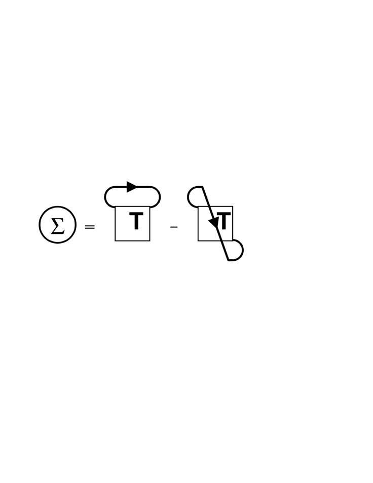
Figure 2: The normal part of the self-energy in the $T-$matrix approximation.

The self-energy can be defined generalizing the self-energy in the $T$-matrix approximation for the normal phase. The diagonal part of the self-energy is defined by the $T$-matrix approximation to the two-particle Green’s function (Fig. 2)

$${\Sigma}^{<>}_{TM}(p,\omega)=i\int\frac{d\omega^{{}^{\prime}}}{2\pi}\frac{d^{3}k}{(2\pi)^{3}}\langle{\bf(p-k)}/2|T_{A}^{<>}(\omega+\omega^{{}^{\prime}},{\bf p+k})|{\bf(p-k)}/2\rangle G^{<>}(k,\omega^{{}^{\prime}})\ \ .$$ (30)

Analogously we can define the $T$-matrix part of the off-diagonal self-energy (Fig. 3)

$${\Delta}^{<>}_{TM}(p,\omega)=i\int\frac{d\omega^{{}^{\prime}}}{2\pi}\frac{d^{3}k}{(2\pi)^{3}}\langle{\bf(p-k)}/2|L_{A}^{<>}(\omega+\omega^{{}^{\prime}},{\bf p+k})|{\bf(p-k)}/2\rangle F^{<>}(k,\omega^{{}^{\prime}})\ \ .$$ (31)

The above definition of self-energy is a $\Phi$-derivable approximation [40] (Fig. 4). It leads to thermodynamically consistent results. In Eqs. (31) and (30) the subscript _A denotes the antisymmetrization and we have not written explicitely the spin-isospin indices. It can be checked that the formula (31) conserves the singlet (triplet) structure of the order parameter given by $F$. The approximation (31) does not include the usual BCS part of the anomalous self-energy

$$\Delta_{BCS}(p)=-i\int\frac{d\omega}{2\pi}\int\frac{d^{3}k}{(2\pi)^{3}}V(p,k)F^{<}(k,\omega)\ \ .$$ (32)

This term can be added explicitely to the the off-diagonal part of the self-energy (Fig. 3). Moreover the $\Phi$ derivability of the approximation is conserved. As it will turn out the BCS part of the anomalous self-energy is dominant, and in the first approximation one can neglect the two-body contribution (31) to the superfluid gap. However the approximation scheme consisting in keeping the $T$-matrix form of the diagonal self-energy and the BCS form of the off-diagonal self-energy is not $\Phi$-derivable.

2.5 Quasi-particle approximation

The full solution of the set of equations (2.3) for the generalized $T$-matrix, the normal self-energy and the superfluid gap requires a self-consistent iterative solution. Below we present results of a simpler calculation. It starts with the mean field approximation for the normal self-energy (Hartree-Fock approximation) and the BCS approximation for the superfluid gap

$$\Delta_{BCS}(p)=-\int\frac{d^{3}k}{(2\pi)^{3}}V(p,k)\frac{\left(1-2f(E_{k})\right)}{2E_{k}}\Delta_{BCS}(k)\ .$$ (33)

The starting spectral function for the calculation of the $T$-matrix is

$$A_{BCS}(p,\omega)=2\pi\left(\frac{E_{p}+\xi_{p}}{2E_{p}}\delta(\omega-E_{p})+\frac{E_{p}-\xi_{p}}{2E_{p}}\delta(\omega+E_{p})\right)$$ (34)

where $\xi_{p}=p^{2}/2m+\Sigma_{HF}(p)-\mu$ and $E_{p}=\sqrt{\xi_{p}^{2}+\Delta_{p}^{2}}$. The corresponding off-diagonal spectral function is

$$B(p,\omega)=-2\pi\frac{\Delta_{p}}{2E_{p}}\left(\delta(\omega-E_{p})-\delta(\omega+E_{p})\right)\ .$$ (35)

The generalized $T$-matrix equation is solved for the $S$-wave Yamaguchi interaction [41]. This oversimplified interaction is used to reduce the numerical difficulties involved in the solution of $T$-matrix equations and in the calculation of the self-energies. First the imaginary parts of the diagonal and off-diagonal self-energies are calculated

$${\rm Im}\Sigma(p,\omega)=\int\frac{d^{3}k}{(2\pi)^{3}}\left(\frac{E_{p}+\xi_{p}}{2E_{p}}\left(f(E_{p})+b(\omega+E_{p})\right)\right.$$

$$\langle({\bf p-k})/2|{\rm Im}T({\bf p+k},\omega+E_{p})|({\bf p-k})/2\rangle_{A}$$

$$\left.+\frac{E_{p}-\xi_{p}}{2E_{p}}\left(f(-E_{p})+b(\omega-E_{p})\right)\langle({\bf p-k})/2|{\rm Im}T({\bf p+k},\omega-E_{p})|({\bf p-k})/2\rangle_{A}\right)$$ (36)

and similarly for ${\rm Im}\Delta_{TM}$ ($b(\omega)$ is the Bose distribution). Then from the dispersion relations the real part of the dispersive contribution to the self-energy can be obtained

$$\left(\matrix{{\rm Re}\Sigma(p,\omega)_{disp}\cr{\rm Re}\Delta(p,\omega)_{TM}}\right)={\cal P}\int\frac{d\omega^{{}^{\prime}}}{2\pi}\left(\matrix{{\rm Im}\Sigma(p,\omega^{{}^{\prime}})_{disp}\cr{\rm Im}\Delta(p,\omega^{{}^{\prime}})_{TM}}\right)\frac{1}{\omega-\omega^{{}^{\prime}}}\ .$$ (37)

To the dispersive part of the self-energies one has to add the mean-field self-energy $\Sigma_{HF}$ and the mean field superfluid gap $\Delta_{BCS}$

$${\rm Re}\Sigma(p,\omega)={\rm Re}\Sigma(p,\omega)_{disp}+\Sigma_{HF}(p)$$

$${\rm Re}\Delta(p,\omega)={\rm Re}\Delta(p,\omega)_{TM}+\Delta_{BCS}(p)$$ (38)

that have been calculated already to obtain the spectral functions (34), (35).

3 Results for the $T$-matrix

3.1 Energy gap in the $T$-matrix and the two-particle spectral function

The equations for the generalized $T$-matrix are solved with the quasi-particle ansatz for the spectral functions $A$ and $B$. We present results at the temperature of $3$MeV with the BCS gap of $10.1$MeV. The results do not change appreciably when reducing the temperature further. In Fig 5 is shown the imaginary part of the diagonal and off-diagonal parts of the generalized $T$-matrix. From the BCS ansatz for the spectral functions follows a gap in two-particle excitations around the the Fermi energy. For zero total momentum of the pair, this forbidden region is twice the superfluid gap. At the edge of the two-particle gap the generalized $T$-matrix has a singularity as function of energy, similar to the singularities in the one-particle spectral function in the BCS approximation.

In fact the imaginary part of the $T$-matrix is related to the two-particle propagator in the $T$-matrix approximation. The one-time two-particle spectral function is

$$\left(\matrix{\langle{p}|A_{2}({P},\Omega)|{p^{{}^{\prime}}}\rangle&\langle{p}|B_{2}({P},\Omega)|{p^{{}^{\prime}}}\rangle\cr\langle{p}|B_{2}({P},-\Omega)|{p^{{}^{\prime}}}\rangle&\langle{p}|A_{2}({P},-\Omega)|{p^{{}^{\prime}}}\rangle}\right)=$$

$$-2{\rm Im}\int\frac{d^{3}q}{(2\pi)^{3}}\int\frac{d^{3}k}{(2\pi)^{3}}\left(\matrix{V^{-1}({p},{p^{{}^{\prime}}})&0\cr 0&V^{-1}({p},{p^{{}^{\prime}}})}\right)$$

$$\left(\matrix{\langle{q}|T^{\pm}({P},\Omega)|{k}\rangle&\langle{q}|L^{\pm}({P},\Omega)|{k}\rangle\cr\langle{q}|L^{\pm}({P},-\Omega)|k\rangle&\langle{q}|T^{\pm\dagger}({P},-\Omega)|k\rangle}\right)\left(\matrix{V^{-1}({k},{p^{{}^{\prime}}})&0\cr 0&V^{-1}({k},{p^{{}^{\prime}}})}\right)$$ (39)

The spin-isospin indices are omitted, and the two-particle spectral function can be projected on a definite total spin or isospin of the pair. Also the relative momentum can be projected on states with definite angular momentum. In Fig. 6 we present the two particle spectral function projected on partial waves occurring in our separable interaction

$$\langle A_{2}(P,\Omega)\rangle=\int\frac{d^{3}kd^{3}p}{(2\pi)^{6}}g(k)g(p)\langle k|A_{2}(P,\Omega)|p\rangle\ ,$$ (40)

where $g(k)=1/(k^{2}+\beta^{2})$ is the formfactor of the Yamaguchi interaction [41]. We use the same projection for the off-diagonal two-particle spectral function $B_{2}$ in different channels and for the uncorrelated BCS two-particle propagators.

The energy gap present in the two-particle BCS propagator is visible also in the $T$-matrix approximation (Fig. 6). It corresponds to a minimal energy to excite a two-particle pair of twice the single-particle energy gap. A similar gap appears in the two-particle anomalous propagator (Fig. 7) and for nonzero momentum of the pair (Figs. 8, 9).

3.2 Singularity in the $T$-matrix

The $T$-matrix is singular for the total energy of the pair equal to twice the Fermi energy and zero total momentum. It is a generalization of the Thouless criterion for the critical temperature to the superfluid phase. Indeed the imaginary part of $T$ and $L$ is always zero at $\Omega=0$ and $P=0$ and the inverse of the real part of the generalized $T$-matrix

$${\rm Re}\langle k^{{}^{\prime}}|\left(\matrix{T&L\cr L&T^{\dagger}}\right)_{P=0,\Omega=0}|k\rangle^{-1}$$ (41)

has a zero eigenvalue

$$\int d^{3}k\langle k^{{}^{\prime}}|\left(\matrix{T&L\cr L&T^{\dagger}}\right)_{P=0,\Omega=0}|k\rangle^{-1}\left(\matrix{\Delta(k)\cr-\Delta(k)}\right)=0\ .$$ (42)

$\Delta(k)$ (with spin-isospin indices omitted) is a solution of the mean-field gap equation

$$\Delta(p)-\int\frac{d^{3}k}{(2\pi)^{3}}V(p,k)\frac{d\omega d\omega^{{}^{\prime}}}{(2\pi)^{2}}\frac{A(\omega,k)A_{s}(\omega,k)}{\omega+\omega^{{}^{\prime}}}\left(1-f(\omega)-f(\omega^{{}^{\prime}}\right))\Delta(k)=0$$ (43)

if $A_{s}$ is the full spectral function with only the BCS contribution to the off-diagonal self-energy $\Delta_{BCS}$. In particular the inverse generalized $T$-matrix with mean-field quasi-particle propagators (34), (35) has a zero eigenvalue corresponding to the BCS mean-field superfluid gap (33). In Fig. 10 is shown the real part of the inverse determinant of the generalized $T$-matrix for the two $S$ partial waves. Clearly the superfluid gap is formed in the ${}^{3}S_{1}$ channel (for the chosen interaction). The generalized $T$-matrix in this channel shows a singularity at zero total momentum and at twice the Fermi energy for all temperatures below $T_{c}$.

4 Self-energies and spectral functions

4.1 Single-particle energies

The position of the single particle pole $\omega_{p}$ when including only the real part of the self-energy can be obtained from the solution of

$$\omega_{p}=\frac{p^{2}}{2m}+{\rm Re}\Sigma(p,\omega_{p})-\mu\ .$$ (44)

In Fig. 11 it is compared to the position of the quasi-particle pole $\xi_{p}$ when including only the Hartree-Fock self-energy. There is a significant difference between the mean-field single-particle energy and the single-particle energy (44) for low-momenta, due to the dispersive part of the self-energy as obtained in the $T$-matrix approximation. It is a reflection of the presence of short range correlations for nuclear interactions. This modification of single-particle energies below the Fermi energy leads to important corrections to the binding energy per particle in nuclear matter. A resummation of ladder diagrams in the form of the $G$-matrix (or the $T$-matrix) is necessary to obtain reliable results for the binding energy [42, 21].

In the superfluid the presence of the off-diagonal self-energy $\Delta(p,\omega)$ leads to the splitting of quasi-particle poles in the spectral function $A_{s}(p,\omega)$

$$E_{p}=\pm\sqrt{(\xi_{p}+{\rm Re}\Sigma(p,E_{p}))^{2}+|\Delta(p,E_{p})|^{2}}\ .$$ (45)

As shown in Fig. 11 the superfluid quasi-particles, present a gap in excitations around the Fermi momentum. Far from from the Fermi momentum the dominant quasi-particle pole of $A_{s}(p,\omega)$ approaches the quasi-particle pole $\omega_{p}$ of $A(p,\omega)$. In Fig. 12 the position of the quasi-particle poles obtained including the full off-diagonal self-energy (Eq. 45) is compared to one where only the BCS part of the superfluid gap is taken

$$E_{p}=\pm\sqrt{(\xi_{p}+{\rm Re}\Sigma(p,E_{p}))^{2}+|\Delta_{BCS}(p)|^{2}}\ .$$ (46)

The two energies are very close. At the scale of Fig. 11 they cannot be distinguished and only close to the Fermi momentum a small difference can be seen in Fig. 12. It is due to the fact that the dispersive part of the off-diagonal self-energy $\Delta_{TM}(p,\omega)$ introduces only a small correction to the mean-field superfluid gap $\Delta_{BCS}(p)$.

4.2 Imaginary part of the self-energy

In Fig. 13 we plot the energy dependence of $-{\rm Im}\Sigma^{+}(p,\omega)$ for several values of the momentum $p$. A characteristic feature is the very strong reduction of the damping in the region around the Fermi energy, already at $T=3$MeV. It is related to the appearance of an energy gap for excitations of twice the value of the superfluid gap. On top of that the usual reduction of damping due to the restriction of the phase space appears, leading to the formation of quasi-particles around the Fermi surface.

The quasi-particle nature of the excitations can be judged by plotting the single particle width

$$\Gamma(\omega,p)=-2{\rm Im}\Sigma(p,\omega)\$$ (47)

at the quasi-particle pole. The single particle width is small around the Fermi energy for the quasi-particle pole $\omega=\omega_{p}$ and the poles $\omega=\pm E_{p}$ (Fig. 14). The formation of the energy gap for excitation of particle pairs and the reduction of the phase space around the Fermi surface leads to the appearance of sharp quasi-particles for momenta close to the Fermi momentum.

4.3 Superfluid gap

The superfluid gap acquires a contribution $\Delta_{TM}$ from the $T$-matrix diagram. The real part of the $T$-matrix gap is obtained from the dispersion relation (37). In Fig. 15 is shown ${\rm Re}\Delta_{TM}(p,\omega)$ for several values of momenta. Its value is small for energies corresponding to the Fermi energy and for momenta close to the Fermi momentum.

In Fig. 16 is shown the imaginary part of the $T$-matrix contribution to the superfluid gap. The imaginary part of the dispersive contribution to the superfluid gap ${\rm Im}\Delta_{TM}(p,\omega)$ shows a gap around the Fermi energy similarly as the imaginary part of the diagonal self-energy. This means that the imaginary part is not modifying the value of the superfluid gap around the Fermi surface.

In Fig. 17 the mean-field superfluid gap $\Delta_{BCS}(p)$ is compared to the superfluid gap containing also the $T$-matrix contribution at the quasi-particle poles $\omega_{p}$ or $E_{p}$. Close to the Fermi momentum the mean-field value of the superfluid gap is not modified significantly. Only for small momenta the $T$-matrix contribution to $\Delta(p,E_{p})$ shows up.

4.4 Spectral functions

The quasi-particle nature of the excitations around the Fermi momentum can be judged from the spectral functions $A(p,\omega)$ and $A_{s}(p,\omega)$. In the upper panel of Fig. 18 are shown the spectral functions for $p=0$ (below the Fermi surface). The main strength of the spectral function is concentrated around the quasi-particle peak at $\omega=-56{\rm MeV}=\omega_{p}\simeq-E_{p}$. However for this momentum the spectral function is relatively spread. The quasi-particle approximation would be of limited validity. Above the Fermi energy the strength of the spectral function is small. It is slightly larger for $A_{s}$ than for $A$ because of the contribution of the second quasi-particle pole of the full spectral function $A_{s}(p,\omega)$ in the superfluid.

The situation is reversed in the lower panel of Fig. 18 where the spectral functions are plotted for the momentum $p=350$MeV (above the Fermi momentum). The quasi-particle pole of $A$ and the dominant quasi-particle pole of $A_{s}$ are located above the Fermi energy. Below the Fermi energy there is a small contribution from the background strength of the spectral function to $A$ and $A_{s}$ and a small contribution from the second pole to the full spectral function $A_{s}$.

In the middle panel of Fig 18 are shown the spectral functions for a momentum close to the Fermi momentum. Very sharp quasi-particle peaks are visible for $A(p,\omega)$ at $\omega=\omega_{p}$ and for $A_{s}(p,\omega)$ at $\omega=\pm E_{p}$. For this momentum the difference between $A$ and $A_{s}$ is the most pronounced, because $\omega_{p}$ is different from $E_{p}$ and both poles of $A_{s}$ have comparable strength.

In Fig. 19 is plotted the off-diagonal spectral function $B(p,\omega)$. The anomalous spectral function is an odd function of energy. $B(p,\omega)$ has two quasi-particle poles on both sides of the Fermi energy. The quasi-particle poles are very sharp for momenta close to the Fermi momentum. Only for small momenta the off-diagonal spectral function shows two relatively broad peaks.

5 Conclusions

We present an approach which allows for the resummation of ladder diagrams in the form of the in-medium $T$-matrix and the treatment of the superfluid phase of the nuclear matter at the same time. The approximation presented in Sect. 2.3 is a generalization of the usual $T$-matrix resummation in medium to temperatures below $T_{c}$. In the superfluid phase the Green’s functions, self-energies and the $T$-matrix acquire additional indices corresponding to anomalous propagators. The approach is $\Phi$-derivable and hence it is thermodynamically consistent, like the self-consistent $T$-matrix approximation. The partial wave expansion can be performed for central forces. The corresponding self-energy is calculated assuming the $T$-matrix approximation for the two-particle propagator and the two-particle anomalous propagator. The off-diagonal self-energy can be supplemented with the mean-field BCS contribution which turns out to be dominant. The addition of the BCS gap to the off-diagonal self-energy does not spoil the $\Phi$ derivability of the approximation. The spin-isospin structure of the $T$-matrix part of the superfluid order parameter is the same as its mean-field part.

In this exploratory work we use a simple separable interaction to illustrate the method by numerical results. The calculations are performed in the approximation where the normal and anomalous propagators in the generalized $T$-matrix ladder and in the self-energy diagrams are of the BCS mean-field form. It represents the first iteration in the calculation of the self-consistent set of equations with off-shell normal and anomalous propagators. It turns out that the real part of the diagonal self-energy changes in the first iteration significantly from its mean-field form. On the other hand the value of the superfluid gap is only slightly modified by the addition of the $T$-matrix contribution in the first iteration. The imaginary part of the diagonal self-energy is reduced around the Fermi energy due to the appearance of an energy gap for excitation of twice the value of the superfluid gap. The quasi-particle approximation is a reasonable description of excitations close to the Fermi surface, with single-particle energies modified by the resummation of ladder diagrams.

Let us comment on the influence of the use of more realistic forces on the results. The importance of the ladder diagram resummation for the real-part of the self-energy is of course important for any realistic interactions [42, 21, 32, 36, 26]. The value of the superfluid gap is expected to be much smaller for realistic nuclear potentials at normal nuclear density. The validity of the partial wave expansion for non-central forces in the superfluid remains to be checked. However since we expect that the dominant part of the off-diagonal self-energy comes from BCS diagram the partial wave expansion in the generalized $T$-matrix calculation would not introduce important modifications for final self-energies.

Another open question is the effect of the self-consistency of the calculation on the spectral functions and self-energies. The equations for the self-energies and the generalized $T$-matrix should be iterated instead of using only the quasi-particle mean-field propagators. In the self-consistent iteration the superfluid gap is reduced [12] and the energy gap in the superfluid is no longer sharp. The imaginary part of the self-energy will also be reduced around the Fermi energy but not as sharply as in Fig. 14. We note that only the use of self-consistent propagators and self-energies in the generalized $T$-matrix approximation guarantees the thermodynamic consistency of the results [27]. As a result of the self-consistency in the off-diagonal self-energy the generalized $T$-matrix will not have a singularity at twice the Fermi energy and zero total momentum. As described in Sect. 3.2 this singularity is present only if mean-field BCS off-diagonal self-energy is used in propagators of the ladder. The inclusion of two-particle contribution to the order parameter modifies this criterion for long range order in the two-particle propagator.

Finally comparing to results of Ref. [23] we found a similar behavior of the real part of the generalized $T$-matrix if using BCS propagators, i.e. a singularity at twice the Fermi energy and zero total momentum. However the imaginary part of the $T$-matrix is very different form the results in Ref. [23]. The generalized $T$-matrix approximation shows an excitation gap around the Fermi energy, which leads to similar gaps in the one-particle and two-particle spectral functions. This feature is very comforting since it is a manifestation of the energy gap for the excitation of particle pairs present in the superfluid.

This work was partly supported by the KBN under Grant 2P03B02019.

Figure 1: The generalized $T$-matrix equation in the superfluid.

Figure 3: The off-diagonal part of the self-energy in the generalized $T-$matrix approximation with the BCS contribution.

Figure 4: Diagrams contributing to the generating functional $\Phi$ in the generalized $T-$matrix approximation.

Figure 5: Imaginary part of the diagonal (solid line) and off-diagonal (dashed line) part of the generalized $T$-matrix in the ${}^{3}S_{1}$ channel

.

Figure 6: Two-body spectral function for normal propagators obtained form the generalized $T$-matrix (solid line) and from two uncorrelated BCS propagators (dashed line). Projected on the ${}^{3}S_{1}$ channel (upper panel) and ${}^{1}S_{0}$ channel (lower panel).

Figure 7: Two-body spectral function for anomalous propagators obtained form the generalized $T$-matrix (solid line) and from two uncorrelated BCS anomalous propagators (dashed line). Projected on the ${}^{3}S_{1}$channel (upper panel) and ${}^{1}S_{0}$ channel (lower panel).

Figure 8: Two-body spectral function for normal propagators obtained form the generalized $T$-matrix (solid line) and from two uncorrelated BCS propagators (dashed line) for nonzero total momentum of the pair ($P=525$MeV), projected on the ${}^{3}S_{1}$ channel.

Figure 9: Two-body spectral function for anomalous propagators obtained form the generalized $T$-matrix (solid line) and from two uncorrelated BCS anomalous propagators (dashed line) for nonzero total momentum of the pair ($P=525$MeV), projected on the ${}^{3}S_{1}$ channel.

Figure 10: Real part of the determinant of the inverse $T$-matrix for the ${}^{3}S_{1}$ (solid line) and the ${}^{1}S_{0}$ channel (dashed line).

Figure 11: The position of the quasi-particle pole for normal self-energy for the HF propagator (solid line) and for the propagator including the normal self-energy from the $T$-matrix calculation (dashed line). The positions of quasi-particle poles of the full propagator including the normal and the off-diagonal self-energies in the $T$-matrix approximation are denoted by the dotted lines.

Figure 12: The positions of quasi-particle poles of the full propagator including the normal and the off-diagonal self-energies in the $T$-matrix approximation are denoted by the dashed lines. The solid line represents the positions of the poles when taking the BCS form only for the off-diagonal self-energy.

Figure 13: The imaginary part of the retarded self-energy as function of energy for $p=0,140,280,420$MeV (solid, dashed, dotted, dash-dotted lines).

Figure 14: The single-particle width at the quasi-particle pole of $A(p,\omega)$ (solid line) and at the quasi-particle poles of $A_{s}(p,\omega)$ (dashed lines).

Figure 15: The real part of the $T$-matrix contribution to the superfluid gap as function of energy for $p=0,116,233,350$MeV (solid, dashed, dotted and dash-dotted lines).

Figure 16: The imaginary part of the $T$-matrix contribution to the superfluid gap as function of energy for $p=0,116,233,350$MeV (solid, dashed, dotted and dash-dotted lines).

Figure 17: The value of the superfluid gap at the quasi-particle pole of $\omega_{p}$ (dotted line) and at the pole $E_{p}$ (dashed line) compared to the BCS gap (solid line).

Figure 18: The spectral function $A(p,\omega)$ including only the diagonal self-energy (solid lines) and the full spectral function $A_{s}(p,\omega)$ (dashed lines) as function of the energy.

Figure 19: The off-diagonal spectral function $B(p,\omega)$ for $p=0,280$ and $350$MeV (dotted, solid and dashed lines respectively).

References

- [1] B.E. Vonderfecht, C.C. Gerhart, H.H. Dickhoff, A. Polls and A. Ramos, Phys. Lett. B253, 1 (1991).
- [2] M. Baldo, I. Bombaci and U. Lombardo, Phys. Lett. B283, 8 (1992).
- [3] M. Baldo, U. Lombardo and P. Schuck, Phys. Rev. C52, 975 (1995).
- [4] U. Lomabrdo and P. Schuck, Phys. Rev. C63, 038201 (2001).
- [5] H. Kucharek, P. Ring, P. Schuck and R. Bengston, Phys. Lett. B216, 249 (1989); P. Schuck and K. Taruishi, Phys. Lett. B385, 12 (1996); E. Garrido, P. Sarriguen, E. Moya de Guerra and P. Schuck, Phys. Rev. C60, 064312 (1999); E. Garrido, P. Sarriguren, E. Moya de Guerra, U. Lombardo , P. Schuck and H.-J. Schulze, Phys. Rev. C63, 037304 (2001).
- [6] A.L. Goodman, Phys. Rev. C58, 3051, (1998); ibid C60, 014311 (1999).
- [7] G. Röpke, A. Schnell, P. Schuck and U. Lombardo, Phys. Rev. C61, 024306 (2000).
- [8] W. Satuła and R. Wyss, Phys. Lett. B393, 1 (1997); W. Satuła, D.J. Dean, J. Gary, S. Mizutori and W. Nazarewicz, Phys. Lett. B407, 103 (1997).
- [9] J.W. Clark, C.-G. Källman, C.-H. Yang and D.A. Chakkalakal, Phys. Lett B61, 331 (1976).
- [10] T.L. Ainsworth, J. Wambach and D. Pines, Phys. Lett. B222, 173 (1989); J. Wambach, T.L.Ainsworth and D. Pines, Nucl. Phys. A555, 128 (1993).
- [11] H.-J. Schulze, J. Cugnon, A. Lejeune, M. Baldo and U. Lombardo, Phys. Lett. B375, 1 (1996); H.-J. Schulze, A. Polls and A. Ramos, Phys. Rev. C63, 044310 (2001).
- [12] P. Bożek, Phys. Rev. C62, 054316 (2000).
- [13] M. Baldo and A. Grasso, Phys. Lett B485, 115 (2000).
- [14] U. Lombardo, P. Schuck and W. Zuo, Phys. Rev. C64, 021301 (2001).
- [15] D. Pines and M.A. Alpar, Nature 316, 27 (1985); K.A. Van Riper, B. Link and R.I. Epstein, Astrophys. J. 448, 294 (1995); S. Tsuruta, Phys. Rep. 292, 1 (1998).
- [16] M. Baldo, J. Cugnon, A. Lejeune and U. Lombardo, Nucl. Phys. A515, 409 (1990); ibid A536, 349 (1992).
- [17] Ø. Elgarøy, L. Engvik, M. Hjorth-Jensen and E. Osnes, Nucl Phys. A604, 466 (1996); F.V. De Blasio, M. Hjorth-Jensen, Ø. Elgarøy, L. Engvik, G. Lazzari, M. Baldo and H.-J. Schulze, Phys. Rev. C56, 2332 (1997); M. Baldo, Ø. Elgarøy, L. Engvik, M. Hjorth-Jensen and H.-J. Schulze, Phys. Rev. C58, 1921 (1998).
- [18] T. Alm, G. Röpke, A. Sedrakian and F. Weber, Nucl. Phys. A604, 491 (1996); A. Sedrakian, T. Alm and U. Lombardo, Phys. Rev. C55, 582 (1997).
- [19] A. Sedrakian and U. Lombardo, Phys. Rev. Lett. 84, 602 (2000); U.Lombardo, P. Noziére, P. Schuck, H.-J. Schulze and A. Sedriakan, nucl-th/0109024.
- [20] T. Alm, B.L. Friman, G. Röpke and H. Schulz, Nucl. Phys. A551, 45 (1993).
- [21] A.L. Fetter, J.D. Walecka, Quantum Theory of Many-Particle Systems, (McGraw-Hill, New York, 1971).
- [22] L.N. Cooper, Phys. Rev. 104, 1189 (1956).
- [23] P. Bożek, Nucl. Phys. A657, 187 (1999).
- [24] W.H. Dickhoff, Phys. Rev. C58, 2807 (1998).
- [25] W.H. Dickhoff, C.C. Gearhart, E.P. Roth, A. Polls and A. Ramos, Phys. Rev. C60, 064319 (1999).
- [26] P. Bożek, Phys. Rev. C59, 2619 (1999).
- [27] P. Bożek and P. Czerski, nucl-th/0102020.
- [28] Y. Dewulf, D. Van Neck and M. Waroquier, Phys. Lett. B510, 89 (2001).
- [29] G. Röpke and A. Schnell, Prog. Part. Nucl. Phys. 42, 53 (1999).
- [30] B.E. Vonderfecht, W.H. Dickhoff, A. Polls and A. Ramos, Nucl. Phys. A555, 1 (1993), ibid. Phys. Rev. C44, 1265 (1991).
- [31] P. Bożek, Workshop on Kadanoff-Baym Equations: Progress and perspectives for Many-Body Physics, Rostock 1999, ed. M. Bonitz, (World Sci., Singapore, 2000).
- [32] T. Alm, G. Ropke, A. Schnell, N.H. Kwong and H.S. Kohler, Phys. Rev. C 53, 2181 (1996).
- [33] A. Schnell, T. Alm and G. Röpke, Phys. Lett. B387, 443 (1996).
- [34] N.M. Hugenholz and L. Van Hove, Physica 24, 363 (1958).
- [35] T. Alm, G. Röpke and M. Schmidt, Phys. Rev. C50, 31 (1994).
- [36] A. Schnell, G. Ropke and P. Schuck, Phys. Rev. Lett. 83, 1926 (1999).
- [37] L.V. Keldysh, Sov. Phys. JETP 20, 235 (1965).
- [38] J.R. Schrieffer, Theory of Superconductivity, (W.A. Benjamin, Inc. New York, 1965).
- [39] R. Hausmann, Phys. Rev. B49, 12975 (1994); R. Hausmann, Z. Phys. B91, 291 (1993); M.H. Pedersen, J.J. Rodríguez-Núñez, H. Beck, T. Schneider and S. Schafroth, Z. Phys. B103, 21 (1997).
- [40] J.M. Luttinger and J.C. Ward, Phys. Rev. 118 1417 (1960); G. Baym, Phys. Rev. 127 1392 (1962); L.P. Kadanoff and G. Baym, Quantum Statistical Mechanics (Benjamin, New York, 1962).
- [41] Y. Yamaguchi, Phys. Rev. 95, 1628 (1954).
- [42] B.D. Day, Rev. Mod. Phys. 39, 719 (1967).
.