A method of implementing Hartree-Fock calculations with zero- and finite-range interactions

We develop a new method of implementing the Hartree-Fock calculations. A class of Gaussian bases is assumed, which includes the Kamimura-Gauss basis-set as well as the set equivalent to the harmonic-oscillator basis-set. By using the Fourier transformation to calculate the interaction matrix elements, we can treat various interactions in a unified manner, including finite-range ones. The present method is numerically applied to the spherically-symmetric Hartree-Fock calculations for the oxygen isotopes with the Skyrme and the Gogny interactions, by adopting the harmonic-oscillator, the Kamimura-Gauss and a hybrid basis-sets. The characters of the basis-sets are discussed. Adaptable to slowly decreasing density distribution, the Kamimura-Gauss set is suitable to describe unstable nuclei. A hybrid basis-set of the harmonic-oscillator and the Kamimura-Gauss ones is useful to accelerate the convergence, both for stable and unstable nuclei.

PACS numbers: 21.60.Jz, 21.30.Fe, 21.10.Gv, 27.30.+t

Keywords: Hartree-Fock calculation, unstable nuclei, density distribution, finite-range interaction

1 Introduction

Since the invention of the secondary beam technology, numerous experimental data on the unstable nuclei have disclosed new aspects of the atomic nuclei. Remarkable examples are the presence of the nuclear halos and skins, and the dependence of magic numbers on the neutron (or proton) excess [1]. It should be noticed that both are closely related to the properties of the single-particle (s.p.) orbits in the unstable nuclei. In order to understand these new phenomena, which have raised questions on some of our conventional picture of the nuclear structure, it is worthwhile reinvestigating the properties of the s.p. orbits in nuclei.

Because the atomic nuclei are bound without an external field, a mean-field is necessary to obtain the s.p. orbits. The Hartree-Fock (HF) theory and its extensions, which are self-consistent approaches, will be a desirable tool to investigate the s.p. orbits from microscopic standpoints. In studying the structure of unstable nuclei, it is a practical problem how to treat numerically the wave-functions at relatively large $r$, because there may be a halo. Most of the methods employed so far are adapted to the nuclei with sharply decreasing densities at the surface. They are not necessarily eligible to reproduce the halo structure. Furthermore, an important physics problem lies in the effective interaction. Not many effective interactions have been used in the HF calculations of nuclei. The Skyrme interaction [2] has been popular in the HF studies, since the zero-range form is easy to be handled. A number of parameter-sets have been proposed for the Skyrme interaction. In the Skyrme interaction the non-locality in the nuclear interaction is approximated by the momentum dependence of the zero-range force. This approximation was justified by Negele and Vautherin via the density-matrix expansion [3]. However, despite the success for the stable nuclei and its recent development [4], it has not been inspected sufficiently whether the first few terms of the density-matrix expansion give good description of the nuclei far from the $\beta$-stability. In this regard, it is desired to deal also with finite-range interactions. The Gogny interaction [5] is the only finite-range interaction widely applied to the mean-field calculations. In almost all recent studies based on the Gogny interaction, the D1S parameter-set [6] is employed. However, the D1S set has a problem which is revealed in the unstable nuclei [7]. It could be important to consider various possibilities of the effective interactions in the mean-field calculations.

In this article, we develop a new method to implement the HF calculations. The following two points will be kept in mind: (i) for the drip-line nuclei the wave-functions in the asymptotic region could be significant and therefore should be treated properly, and (ii) the method should have capability of handling various effective interactions, particularly some finite-range ones. Satisfying these two conditions, the method developed in this paper will be useful to study structure of unstable nuclei within the HF framework.

2 Single-particle bases

In the following discussions we assume that the s.p. orbits maintain the spherical symmetry, for the sake of simplicity. The extension of the method to the symmetry-breaking cases will be straightforward.

The HF calculations are implemented by solving the s.p. Schrödinger equation (i.e. the HF equation) iteratively. There are two well-known ways to solve the s.p. Schrödinger equation. One is to discretize the radial or spatial coordinate with a finite mesh, and to integrate the differential equation numerically. The other is to introduce a basis-set and to reduce the equation to an eigenvalue problem, by applying the matrix representation to the s.p. Hamiltonian. Unless the effective interaction has zero range, the HF equation becomes an integro-differential equation because the Fock term is non-local. This makes the mesh method to be cumbersome. On the contrary, we can store the two-body matrix elements in the basis method, and then the non-locality in the Fock term addresses no essential difficulty. Since we would deal with finite-range interactions as well as zero-range interactions, it will be advantageous to introduce a certain set of s.p. bases.

Because dimensionality in practical calculations is necessarily finite, the calculated wave-functions more or less inherit characters of the original bases. Therefore the choice of the basis-set is important, and could depend on the system under discussion, in general. The harmonic-oscillator (HO) basis-set has been popular in describing the s.p. orbits of nuclei. However, while the HO set is indeed efficient in the stable nuclei, this is not the case for the drip-line nuclei, as will be shown in Section 5. The density of the drip-line nuclei slowly decreases for large $r$ (radial coordinate). On account of the short-range character of the nuclear force, the asymptotic form of the density distribution should be exponential, $e^{-2\eta r}$ [8], where $\eta=\sqrt{2ME}/\hbar c$ with the separation energy $E$. In the drip-line nuclei, the density in the asymptotic region could sizably contribute to physical quantities such as the rms radius and the binding energy. This is a sharp contrast to the stable nuclei. However, the exponential asymptotics is hardly expressed by the HO bases. It is noticed that the exponent depends on $E$, which is not obtained until the convergence in the HF calculation. We have to reproduce not only the exponential form but also the $E$ dependence of the exponent, for the proper description of the asymptotics. It is commented that, in the mesh method, we need a large number of mesh points to reproduce the density distribution in the asymptotic region, as far as we keep the mesh size uniform.

We consider the s.p. bases having the following form,

$$\varphi_{\alpha\ell jm}({\mathbf{r}}) = R_{\alpha\ell j}(r)[Y^{(\ell)}(\hat{\mathbf{r}})\chi_{\sigma}]^{(j)}_{m}\,;$$

$$R_{\alpha\ell j}(r) = {\cal N}_{\alpha\ell j}r^{\ell+2p_{\alpha}}\exp[-(r/\nu_{\alpha})^{2}]\,.$$ (1)

Here $Y^{(\ell)}(\hat{\mathbf{r}})$ expresses the spherical harmonics and $\chi_{\sigma}$ the spin wave-function. We drop the isospin index without confusion. The index $\alpha$ indicates the extra power of $r$ ($p_{\alpha}$), which is a non-negative integer, and the range of the Gaussian ($\nu_{\alpha}$), simultaneously. The constant ${\cal N}_{\alpha\ell j}$ is determined as

$${\cal N}_{\alpha\ell j}={2^{\ell+2p_{\alpha}+{7\over 4}}\over{\pi^{1\over 4}\sqrt{(2\ell+4p_{\alpha}+1)!!}}}\left({1\over\nu_{\alpha}}\right)^{\ell+2p_{\alpha}+{3\over 2}}\,,$$ (2)

so as for $\langle\varphi_{\alpha\ell jm}|\varphi_{\alpha\ell jm}\rangle$ to be unity. Since the bases of Eq. (1) are non-orthogonal between different $\alpha$’s, the Schrödinger equation leads to a generalized eigenvalue problem when these bases are applied. If we take $p_{\alpha}=0,1,2,\cdots$ with a constant range $\nu_{\alpha}=\nu_{\omega}=\sqrt{2\hbar/M\omega}$, the space spanned by these bases is equivalent to that comprised of the HO bases. Indeed, these bases coincide with the HO ones, whose radial part is given by the associated Laguerre polynomials of $2(r/\nu_{\omega})^{2}$, if the Gram-Schmidt orthogonalization is carried out from the smaller $p_{\alpha}$ to the larger. Because all the HO bases have the common Gaussian factor $e^{-(r/\nu_{\omega})^{2}}$, the superposition of a limited number of the HO bases has the asymptotic form of $e^{-(r/\nu_{\omega})^{2}}$ again. This is the reason why the HO basis-set fails to describe the density (namely, the wave-function) asymptotics of the drip-line nuclei. On the other hand, Kamimura proposed a basis-set [9] in which $\nu_{\alpha}$ is given by a geometric progression, while keeping $p_{\alpha}=0$. This set of bases, which will be called Kamimura-Gauss (KG) basis-set in this article, has been shown to work efficiently in few-body systems [10], including loosely bound ones. Although each KG basis has the Gaussian asymptotics, the exponential decrease of the density at large $r$ is appropriately described to a good approximation by the superposition of the Gaussians with various ranges. The present form of the bases (1) covers both the HO and KG bases.

The form of Eq. (1) allows wider variety of basis-sets than the HO and the KG sets. An immediate possibility is a hybridization of the HO and KG bases. Another possibility may be stochastic selection of $p_{\alpha}$ and $\nu_{\alpha}$, though it is not explored in this paper.

The transformed harmonic-oscillator (THO) bases were developed to reproduce the exponential asymptotics in the density of the loosely bound nuclei, and were applied to the mean-field calculations with the Skyrme interaction [11]. In order to obtain the energy dependence of the exponent, the bases themselves are changed iteratively. It was shown that the THO basis-set gives an improved description of the properties of nuclei near the neutron drip-line, over the HO set. However, in Ref. [11] the actual calculation seems to depend on the characteristics of the zero-range interaction. It might not be easy to deal with finite-range interactions by the THO bases.

The bases of Eq. (1) give the norm matrix of, for each $(\ell,j)$,

$$N^{(\ell j)}_{\alpha\beta} = \langle\varphi_{\alpha\ell jm}|\varphi_{\beta\ell jm}\rangle$$ (3)

$$= {{(2\ell+2p_{\alpha}+2p_{\beta}+1)!!}\over\sqrt{(2\ell+4p_{\alpha}+1)!!(2\ell+4p_{\beta}+1)!!}}\left({\nu_{\beta}\over\nu_{\alpha}}\right)^{p_{\alpha}-p_{\beta}}\left({{2\nu_{\alpha}\nu_{\beta}}\over{\nu_{\alpha}^{2}+\nu_{\beta}^{2}}}\right)^{\ell+p_{\alpha}+p_{\beta}+{3\over 2}}\,.$$

Under the $\ell$ and $j$ conservation, the s.p. Hamiltonian matrix is given by

$$h^{(\ell j)}_{\alpha\beta}=\langle\varphi_{\alpha\ell jm}|\hat{h}|\varphi_{\beta\ell jm}\rangle\,,$$ (4)

where $\hat{h}$ stands for the s.p. Hamiltonian. Suppose that $|\psi_{n\ell jm}\rangle$ is a solution of the s.p. Schrödinger equation,

$$\hat{h}|\psi_{n\ell jm}\rangle=\epsilon_{n\ell j}|\psi_{n\ell jm}\rangle\,.$$ (5)

By expanding $|\psi_{n\ell jm}\rangle$ by the bases $|\varphi_{\alpha\ell jm}\rangle$,

$$|\psi_{n\ell jm}\rangle=\sum_{\alpha}c^{(\ell j)}_{n,\alpha}|\varphi_{\alpha\ell jm}\rangle\,,$$ (6)

the Schrödinger equation (5) is represented as the generalized eigenvalue problem,

$$\sum_{\beta}h^{(\ell j)}_{\alpha\beta}c^{(\ell j)}_{n,\beta}=\epsilon_{n\ell j}\sum_{\beta}N^{(\ell j)}_{\alpha\beta}c^{(\ell j)}_{n,\beta}\,.$$ (7)

Since the norm matrix $N^{(\ell j)}$ is real symmetric, the Cholesky decomposition can be applied, which is equivalent to the orthonormalization of the bases. Then the generalized eigenvalue problem is converted to the normal eigenvalue problem.

When we deal with non-orthogonal bases, we have to be careful for the norm after the orthogonalization not to be too small. In particular, the bases of Eq. (1) could compose an over-complete set, as is obvious from the fact that the HO basis-set, which is equivalent to the set of the bases having a fixed $\nu_{\alpha}$, can already be complete. If the norm after the orthogonalization were too small, i.e. one of the bases were almost linearly-dependent on the other bases, a numerical instability could take place. This condition may pose a practical limit on the present method in choosing $p_{\alpha}$ and $\nu_{\alpha}$.

3 Effective interaction

The effective Hamiltonian for the nuclear mean-field theory consists of the kinetic energy and the effective interaction,

$$H=K+V\,;\quad K=\sum_{i}{{\mathbf{p}}_{i}^{2}\over{2M}}\,,\quad V=\sum_{i<j}v_{ij}\,.$$ (8)

Here $i$ and $j$ are the indices of each nucleon. The s.p. matrix element of the kinetic term is calculated as

$$\langle\varphi_{\alpha\ell jm}|{{\mathbf{p}}^{2}\over{2M}}|\varphi_{\beta\ell jm}\rangle\hskip 298.75394pt$$

$$={1\over{2M\nu_{\alpha}\nu_{\beta}}}\left[(2\ell+2p_{\alpha}+2p_{\beta}+3){{2\nu_{\alpha}\nu_{\beta}}\over{\nu_{\alpha}^{2}+\nu_{\beta}^{2}}}-2\left\{(\ell+2p_{\alpha}){\nu_{\alpha}\over\nu_{\beta}}+(\ell+2p_{\beta}){\nu_{\beta}\over\nu_{\alpha}}\right\}\right.$$

$$\quad\left.+4{{(\ell+2p_{\alpha})(\ell+2p_{\beta})+\ell(\ell+1)}\over{2\ell+2p_{\alpha}+2p_{\beta}+1}}\cdot{{\nu_{\alpha}^{2}+\nu_{\beta}^{2}}\over{2\nu_{\alpha}\nu_{\beta}}}\right]N^{(\ell j)}_{\alpha\beta}\,.$$ (9)

It will be natural to assume the effective interaction $v_{ij}$ to be translationally invariant, except for the density dependence mentioned below.

As stated in Section 1, we would consider various types of the two-body interaction. For the zero-range interaction like the Skyrme force, the s.p. Hamiltonian is represented in terms of the local densities and currents [2, 12]. It is fast to compute the matrix elements of the s.p. Hamiltonian via the local densities and currents. However, this is not the case for finite-range interactions. Hence we shall calculate the two-body interaction matrix elements and store them, as will be discussed in the subsequent section.

The saturation must be fulfilled in the nuclear HF approach. This requires components other than the momentum-independent two-body terms in the central force [13]. A density-dependent (or a three-body) interaction is usually introduced. Because the calculated density is renewed at each HF iteration, it is impractical to store the matrix elements of the density-dependent interaction. We here assume the usual zero-range form for the density-dependent interaction. The contribution of this component to the s.p. Hamiltonian is evaluated via the local densities.

In reproducing the saturation, it could be an alternative way to introduce the momentum dependence in the central force, which satisfies the translational invariance, instead of the density dependence. Although we do not consider that possibility in this paper except for the case of the Skyrme interaction, the momentum-dependent two-body interaction will be handled in a similar manner to the momentum-independent interaction discussed below.

In addition to the saturation properties which are relevant to the central force, the LS splitting is significant in the atomic nuclei. This suggests necessity of the LS and/or the tensor forces, though true origin of the LS splitting is still under discussion [14]. In most mean-field calculations so far, the zero-range LS force was assumed [2, 5]. The zero-range tensor force was sometimes taken into account so as to cancel a certain term of the LS current [15]. Finite-range LS and tensor forces are also considered, as well as the zero-range ones.

We thus consider the effective interaction in the following form,

$$v_{12} = v_{12}^{\rm C}+v_{12}^{\rm LS}+v_{12}^{\rm TN}+v_{12}^{\rm DD}\,;$$

$$v_{12}^{\rm C} = \sum_{\mu}(t_{\mu}^{\rm W}+t_{\mu}^{\rm B}P_{\sigma}-t_{\mu}^{\rm H}P_{\tau}-t_{\mu}^{\rm M}P_{\sigma}P_{\tau})f_{\mu}^{\rm C}(r_{12})\,,$$

$$v_{12}^{\rm LS} = \sum_{\mu}(t_{\mu}^{\rm LSE}P_{\rm TE}+t_{\mu}^{\rm LSO}P_{\rm TO})f_{\mu}^{\rm LS}(r_{12})\,{\mathbf{L}}_{12}\cdot({\mathbf{s}}_{1}+{\mathbf{s}}_{2})\,,$$

$$v_{12}^{\rm TN} = \sum_{\mu}(t_{\mu}^{\rm TNE}P_{\rm TE}+t_{\mu}^{\rm TNO}P_{\rm TO})f_{\mu}^{\rm TN}(r_{12})\,r_{12}^{2}S_{12}\,,$$

$$v_{12}^{\rm DD} = t_{3}(1+x_{3}P_{\sigma})[\rho({\mathbf{r}}_{1})]^{\alpha}\delta({\mathbf{r}}_{12})\,,$$ (10)

where $f_{\mu}$ represents an appropriate function, $\mu$ stands for the parameter attached to the function (e.g. the range of the interaction), and $t_{\mu}$ the coefficient. As examples of $f_{\mu}(r_{12})$, the delta, the Gauss and the Yukawa forms will be considered. The relative coordinate is given by ${\mathbf{r}}_{12}={\mathbf{r}}_{1}-{\mathbf{r}}_{2}$ and $r_{12}=|{\mathbf{r}}_{12}|$. Correspondingly, we define ${\mathbf{p}}_{12}=({\mathbf{p}}_{1}-{\mathbf{p}}_{2})/2$. $P_{\sigma}$ ($P_{\tau}$) denotes the spin (isospin) exchange operator. $P_{\rm TE}$ ($P_{\rm TO}$) is the projection operator on the triplet-even (triplet-odd) two-particle state,

$$P_{\rm TE}={{1+P_{\sigma}}\over 2}\,{{1-P_{\tau}}\over 2}\,,\quad P_{\rm TO}={{1+P_{\sigma}}\over 2}\,{{1+P_{\tau}}\over 2}\,.$$ (11)

Similarly, the projection operators on the singlet states are defined by

$$P_{\rm SE}={{1-P_{\sigma}}\over 2}\,{{1+P_{\tau}}\over 2}\,,\quad P_{\rm SO}={{1-P_{\sigma}}\over 2}\,{{1-P_{\tau}}\over 2}\,.$$ (12)

${\mathbf{L}}_{12}$ is the relative orbital angular momentum,

$${\mathbf{L}}_{12}={\mathbf{r}}_{12}\times{\mathbf{p}}_{12}\,,$$ (13)

${\mathbf{s}}_{1}$, ${\mathbf{s}}_{2}$ are the nucleon spin operators, and $S_{12}$ is the tensor operator,

$$S_{12}=4\,[3({\mathbf{s}}_{1}\cdot\hat{\mathbf{r}}_{12})({\mathbf{s}}_{2}\cdot\hat{\mathbf{r}}_{12})-{\mathbf{s}}_{1}\cdot{\mathbf{s}}_{2}]\,.$$ (14)

The nucleon density is denoted by $\rho({\mathbf{r}})$.

The Skyrme and the Gogny interactions are included in the present category of effective interactions. In the case of the Skyrme interaction, we use $f_{\delta}^{\rm C}(r_{12})=\delta({\mathbf{r}}_{12})$ for the momentum-independent central force. Discussions on the momentum-dependent and LS terms will be given in Appendices A and B. In the case of the Gogny interaction, we set $f_{\mu}^{\rm C}(r_{12})=\exp[-(\mu r_{12})^{2}]$. The LS force has the same form as in the Skyrme interaction. In both interactions, $v_{12}^{\rm TN}=0$ is assumed, except for the counter-term to a part of the LS current. In some of the recent parameterization of the Skyrme interaction [16] the LS contribution is expressed only in the density-functional form, without explicit correspondence to the two-body interactions. They are not expressed in the form of Eq. (10) and will not be considered in this paper.

4 Calculation of two-body interaction matrix elements

We now discuss how to compute the matrix elements of the two-body interactions, $v_{12}^{\rm C}$, $v_{12}^{\rm LS}$ and $v_{12}^{\rm TN}$. Their contribution to $h^{(\ell j)}_{\alpha\beta}$ in Eq. (4) is given by

$$\sum_{n^{\prime}\ell^{\prime}j^{\prime}J}\langle\hat{N}_{n^{\prime}\ell^{\prime}j^{\prime}}\rangle{{2J+1}\over{(2j+1)(2j^{\prime}+1)}}\sum_{\alpha^{\prime}\beta^{\prime}}c^{(\ell^{\prime}j^{\prime})}_{n^{\prime},\alpha^{\prime}}\,c^{(\ell^{\prime}j^{\prime})}_{n^{\prime},\beta^{\prime}}\,\langle(\alpha\ell j,\alpha^{\prime}\ell^{\prime}j^{\prime})J|(v_{12}^{\rm C}+v_{12}^{\rm LS}+v_{12}^{\rm TN})|(\beta\ell j,\beta^{\prime}\ell^{\prime}j^{\prime})J\rangle_{\rm A}\,$$ (15)

where $\langle\hat{N}_{n\ell j}\rangle$ denotes the occupation number of the s.p. orbit. The expression $(\alpha\ell j)$ represents the basis $|\varphi_{\alpha\ell j}\rangle$ of Eq. (1) in Section 2. Though not shown explicitly, the proton-neutron degrees-of-freedom should be considered in Eq. (15), in practice. As has been discussed in the preceding section, the contribution of $v_{12}^{\rm DD}$ to the s.p. Hamiltonian is calculated through the proton and neutron density distributions at each iterative process, as in Ref. [12].

Let us take the central force $v_{12}^{\rm C}$ as an example. The anti-symmetrized two-body matrix element in Eq. (15) is obtained from the non-anti-symmetrized ones,

$$\langle(j^{\prime}_{1}j^{\prime}_{2})J|v_{12}^{\rm C}|(j_{1}j_{2})J\rangle_{\rm A}=\langle(j^{\prime}_{1}j^{\prime}_{2})J|v_{12}^{\rm C}|(j_{1}j_{2})J\rangle-\langle(j^{\prime}_{1}j^{\prime}_{2})J|v_{12}^{\rm C}|(j_{2}j_{1})J\rangle\,,$$ (16)

where $|~{}\rangle_{\rm A}$ ($|~{}\rangle$) denotes anti-symmetrized (non-anti-symmetrized) state vector. Without confusion, the symbol $j$ is regarded as an abbreviation of $(\alpha\ell j)$ and the proton-neutron degrees-of-freedom. As shown in Eq. (15), we only need the anti-symmetrized matrix elements with $\ell_{1}=\ell^{\prime}_{1}$, $\ell_{2}=\ell^{\prime}_{2}$, $j_{1}=j^{\prime}_{1}$ and $j_{2}=j^{\prime}_{2}$ for the spherical HF calculations. However, we here discuss how to evaluate the matrix elements in more general manner, as will be useful in the case that the symmetry is broken. Inserting Eq. (10), we have

$$\langle(j^{\prime}_{1}j^{\prime}_{2})J|v_{12}^{\rm C}|(j_{1}j_{2})J\rangle=\sum_{\mu}\langle(j^{\prime}_{1}j^{\prime}_{2})J|(t_{\mu}^{\rm W}+t_{\mu}^{\rm B}P_{\sigma}-t_{\mu}^{\rm H}P_{\tau}-t_{\mu}^{\rm M}P_{\sigma}P_{\tau})f_{\mu}^{\rm C}(r_{12})|(j_{1}j_{2})J\rangle\,.$$ (17)

Without loss of generality the spatial function $f_{\mu}^{\rm C}(r_{12})$ is assumed to be common for the Wigner, Bartlett, Heisenberg and Majorana terms. The difference among them are in the spin and isospin operators, for which we use the notation ${\cal O}_{\sigma}$ $(=1\mbox{ or }P_{\sigma})$ and ${\cal O}_{\tau}$ $(=1\mbox{ or }P_{\tau})$. By converting the $jj$-coupling to the LS-coupling, each term of the interaction in Eq. (17) is written as

$$\langle(j^{\prime}_{1}j^{\prime}_{2})J|f_{\mu}^{\rm C}(r_{12}){\cal O}_{\sigma}{\cal O}_{\tau}|(j_{1}j_{2})J\rangle\hskip 298.75394pt$$

$$=\sum_{LS}(2L+1)(2S+1)\sqrt{(2j_{1}+1)(2j_{2}+1)(2j^{\prime}_{1}+1)(2j^{\prime}_{2}+1)}\left\{\begin{array}[]{ccc}l_{1}&{1\over 2}&j_{1}\\ l_{2}&{1\over 2}&j_{2}\\ L&S&J\end{array}\right\}\left\{\begin{array}[]{ccc}l^{\prime}_{1}&{1\over 2}&j^{\prime}_{1}\\ l^{\prime}_{2}&{1\over 2}&j^{\prime}_{2}\\ L&S&J\end{array}\right\}$$ (24)

$$\quad\times\langle(l^{\prime}_{1}l^{\prime}_{2})L|f_{\mu}^{\rm C}(r_{12})|(l_{1}l_{2})L\rangle\,\langle{\cal O}_{\sigma}\rangle_{S}\,\langle{\cal O}_{\tau}\rangle\,,\hskip 227.62204pt$$ (25)

where $\langle{\cal O}_{\sigma}\rangle_{S}$ ($\langle{\cal O}_{\tau}\rangle$) denotes the expectation value of ${\cal O}_{\sigma}$ (${\cal O}_{\tau}$) of the spin (isospin) part. The spatial part in the right-hand side is defined by

$$\langle(l^{\prime}_{1}l^{\prime}_{2})L|f_{\mu}^{\rm C}(r_{12})|(l_{1}l_{2})L\rangle=\int d^{3}r_{1}d^{3}r_{2}R_{j^{\prime}_{1}}(r_{1})R_{j^{\prime}_{2}}(r_{2})\{[Y^{(\ell^{\prime}_{1})}(\hat{\mathbf{r}}_{1})Y^{(\ell^{\prime}_{2})}(\hat{\mathbf{r}}_{2})]^{(L)}_{M}\}^{*}$$

$$\times f_{\mu}^{\rm C}(r_{12})R_{j_{1}}(r_{1})R_{j_{2}}(r_{2})[Y^{(\ell_{1})}(\hat{\mathbf{r}}_{1})Y^{(\ell_{2})}(\hat{\mathbf{r}}_{2})]^{(L)}_{M}\,.$$ (26)

The spatial matrix element (26) can straightforwardly be calculated for simple forms of the interaction such as the delta form. However, we here intend to handle various types of interactions, including the Yukawa form. For this purpose, we utilize the Fourier transform of $f_{\mu}(r_{12})$, as was exploited in Ref. [17] for the HO bases.

The Fourier transformation of $f_{\mu}(r_{12})$ gives

$$\tilde{f}_{\mu}(k)=\int d^{3}r_{12}\,f_{\mu}(r_{12})e^{-i{\mathbf{k}}\cdot{\mathbf{r}}_{12}}\,.$$ (27)

By inverting this transformation, we obtain

$$f_{\mu}(r_{12})={1\over{(2\pi)^{3}}}\int d^{3}k\tilde{f}_{\mu}(k)e^{i{\mathbf{k}}\cdot{\mathbf{r}}_{12}}={1\over{(2\pi)^{3}}}\int d^{3}k\tilde{f}_{\mu}(k)e^{i{\mathbf{k}}\cdot{\mathbf{r}}_{1}}e^{-i{\mathbf{k}}\cdot{\mathbf{r}}_{2}}\,.$$ (28)

Substituting Eq. (28) into Eq. (26), we find the ${\mathbf{r}}_{1}$ and ${\mathbf{r}}_{2}$ integrals are separated at the expense of the ${\mathbf{k}}$ integration. The angular integration is implemented by using

$$e^{i{\mathbf{k}}\cdot{\mathbf{r}}}=4\pi\sum_{\lambda}i^{\lambda}(2\lambda+1)j_{\lambda}(kr)\,Y^{(\lambda)}(\hat{\mathbf{k}})\cdot Y^{(\lambda)}(\hat{\mathbf{r}})\,,$$ (29)

where $j_{\lambda}(x)$ denotes the spherical Bessel function, deriving

$$\langle(l^{\prime}_{1}l^{\prime}_{2})L|f_{\mu}^{\rm C}(r_{12})|(l_{1}l_{2})L\rangle=\sum_{\lambda}\sqrt{(2\ell_{1}+1)(2\ell_{2}+1)}\,(\ell_{1}\,0\,\lambda\,0|\ell_{1}^{\prime}\,0)(\ell_{2}\,0\,\lambda\,0|\ell_{2}^{\prime}\,0)$$

$$\times\int_{0}^{\infty}k^{2}dk\,\tilde{f}_{\mu}^{\rm C}(k)\,{\cal I}^{(0)}_{1}(k)\,{\cal I}^{(0)}_{2}(k)\,.$$ (30)

Here ${\cal I}^{(0)}_{1}$ and ${\cal I}^{(0)}_{2}$ are defined as

$${\cal I}^{(0)}_{i}(k)=\int_{0}^{\infty}r^{2}drj_{\lambda}(kr)R_{\alpha_{i}\ell_{i}j_{i}}(r)R_{\alpha^{\prime}_{i}\ell^{\prime}_{i}j^{\prime}_{i}}(r)\,,$$ (31)

with the subscript $i\,(=1,2)$ corresponds to the nucleon index, which actually represents $(\alpha_{i}\ell_{i}j_{i},\alpha^{\prime}_{i}\ell^{\prime}_{i}j^{\prime}_{i})$. Since the radial part of the present basis $R_{\alpha\ell j}(r)$, given in Eq. (1), has the Gaussian form, ${\cal I}^{(0)}(k)$ is calculated analytically,

$${\cal I}^{(0)}(k)=\zeta_{\alpha\ell,\alpha^{\prime}\ell^{\prime}}\,\left({k\over\kappa_{\alpha\alpha^{\prime}}}\right)^{\lambda}\,L^{(\lambda+{1\over 2})}_{{\ell+\ell^{\prime}-\lambda\over 2}+p_{\alpha}+p_{\alpha^{\prime}}}\!\left[\left({k\over\kappa_{\alpha\alpha^{\prime}}}\right)^{2}\right]\,\exp\left[-\left({k\over\kappa_{\alpha\alpha^{\prime}}}\right)^{2}\right]\,,$$ (32)

where $L^{(\alpha)}_{n}(x)$ is the associated Laguerre polynomial and

$$\zeta_{\alpha\ell,\alpha^{\prime}\ell^{\prime}} = {{\displaystyle 2^{{{\ell+\ell^{\prime}}\over 2}+p_{\alpha}+p_{\alpha^{\prime}}}\,\Gamma\left({{\ell+\ell^{\prime}-\lambda}\over 2}+p_{\alpha}+p_{\alpha^{\prime}}+1\right)}\over\sqrt{(2\ell+1)!!(2\ell^{\prime}+1)!!}}\hskip 56.9055pt$$ (33)

$$\hskip 14.22636pt\times\left({\nu_{\alpha^{\prime}}\over\nu_{\alpha}}\right)^{{\ell-\ell^{\prime}\over 2}+p_{\alpha}-p_{\alpha^{\prime}}}\left({{2\nu_{\alpha}\nu_{\alpha^{\prime}}}\over{\nu_{\alpha}^{2}+\nu_{\alpha^{\prime}}^{2}}}\right)^{{\ell+\ell^{\prime}+3\over 2}+p_{\alpha}+p_{\alpha^{\prime}}}\,,$$

$$\kappa_{\alpha\alpha^{\prime}} = 2\sqrt{{1\over\nu_{\alpha}^{2}}+{1\over\nu_{\alpha^{\prime}}^{2}}}\,.$$ (34)

We thus obtain the following expression for the spatial part of the matrix element,

$$\langle(l^{\prime}_{1}l^{\prime}_{2})L|f_{\mu}^{\rm C}(r_{12})|(l_{1}l_{2})L\rangle\hskip 284.52756pt$$

$$=\sum_{\lambda}\sqrt{(2\ell_{1}+1)(2\ell_{2}+1)}\,(\ell_{1}\,0\,\lambda\,0|\ell_{1}^{\prime}\,0)(\ell_{2}\,0\,\lambda\,0|\ell_{2}^{\prime}\,0)\zeta_{\alpha_{1}\ell_{1},\alpha^{\prime}_{1}\ell^{\prime}_{1}}\zeta_{\alpha_{2}\ell_{2},\alpha^{\prime}_{2}\ell^{\prime}_{2}}\hskip 56.9055pt$$

$$\times\int_{0}^{\infty}k^{2}dk\,\tilde{f}_{\mu}^{\rm C}(k)\,\left({k\over\kappa_{\alpha_{1}\alpha^{\prime}_{1}}}\right)^{\lambda}\left({k\over\kappa_{\alpha_{2}\alpha^{\prime}_{2}}}\right)^{\lambda}\,L^{(\lambda+{1\over 2})}_{{\ell_{1}+\ell^{\prime}_{1}-\lambda\over 2}+p_{\alpha_{1}}+p_{\alpha^{\prime}_{1}}}\!\left[\left({k\over\kappa_{\alpha_{1}\alpha^{\prime}_{1}}}\right)^{2}\right]\,\hskip 28.45274pt$$

$$\times\,L^{(\lambda+{1\over 2})}_{{\ell_{2}+\ell^{\prime}_{2}-\lambda\over 2}+p_{\alpha_{2}}+p_{\alpha^{\prime}_{2}}}\!\left[\left({k\over\kappa_{\alpha_{2}\alpha^{\prime}_{2}}}\right)^{2}\right]\,\exp\left[-\left({k\over\kappa_{\alpha_{1}\alpha^{\prime}_{1}}}\right)^{2}-\left({k\over\kappa_{\alpha_{2}\alpha^{\prime}_{2}}}\right)^{2}\right]\,.\quad$$ (35)

Whereas it is not easy in general to evaluate numerically the multi-dimensional integrals to a high precision, we have only one-dimensional $k$ integral in Eq. (35). Moreover, even this $k$ integral is analytically carried out for the typical interaction forms. Recall that the associated Laguerre polynomial is defined as

$$L^{(\alpha)}_{n}(x)=\sum_{q=0}^{n}{{\Gamma(\alpha+n+1)}\over{\Gamma(\alpha+q+1)\,(n-q)!}}\,{x^{q}\over{q!}}\,.$$ (36)

The $k$ integral in Eq. (35) turns out to be the sum of the integrals with the form

$$\int_{0}^{\infty}dk\,k^{2n+2}e^{-(k/\bar{\kappa})^{2}}\tilde{f}_{\mu}(k)\,,$$ (37)

where $n$ is a certain integer and $\bar{\kappa}^{2}=(1/\kappa_{\alpha_{1}\alpha^{\prime}_{1}}^{2}+1/\kappa_{\alpha_{2}\alpha^{\prime}_{2}}^{2})^{-1}$. For the zero-range interaction such as the momentum-independent term of the Skyrme interaction, $f_{\delta}(r_{12})=\delta({\mathbf{r}}_{12})$ leads to $\tilde{f}_{\delta}(k)=1$. Here we substitute $\delta$ for the suffix $\mu$ to show the function form explicitly. The integral of Eq. (37) therefore reduces to

$$\int_{0}^{\infty}dk\,k^{2n+2}e^{-(k/\bar{\kappa})^{2}}={{(2n+1)!!\sqrt{\pi}}\over{2^{n+2}}}\,\bar{\kappa}^{2n+3}\,.$$ (38)

For the Gaussian form such as the Gogny interaction, $f_{\mu}(r_{12})=e^{-(\mu r_{12})^{2}}$ derives $\tilde{f}_{\mu}(k)=({\sqrt{\pi}}/\mu)^{3}\,e^{-(k/2\mu)^{2}}$. Thus the integral of Eq. (37) for the Gauss interaction is

$$\left({\sqrt{\pi}\over\mu}\right)^{3}\int_{0}^{\infty}dk\,k^{2n+2}e^{-(k/\bar{\kappa})^{2}-(k/2\mu)^{2}}=\left({\sqrt{\pi}\over\mu}\right)^{3}{{(2n+1)!!\sqrt{\pi}}\over{2^{n+2}}}\left({1\over{\bar{\kappa}^{2}}}+{1\over{4\mu^{2}}}\right)^{-(n+{3\over 2})}\,.$$ (39)

In both cases the $k$ integral of (37) yields an analytic function. For the Yukawa interaction, $f_{\mu}(r_{12})=e^{-\mu r_{12}}/\mu r_{12}$ leads to $\tilde{f}_{\mu}(k)=4\pi/\mu(\mu^{2}+k^{2})$. The integration of (37) is still written in a compact form, by using the error function,

$${4\pi\over\mu}\int_{0}^{\infty}dk\,{{k^{2n+2}}\over{\mu^{2}+k^{2}}}\,e^{-(k/\bar{\kappa})^{2}}\hskip 227.62204pt$$

$$={{2\pi^{3\over 2}\bar{\kappa}}\over\mu}(-\mu^{2})^{n}\left\{\sum_{r=0}^{n}(2r-1)!!\left(-{{\bar{\kappa}^{2}}\over{2\mu^{2}}}\right)^{r}-{2\mu\over\kappa}\,e^{(\mu/\bar{\kappa})^{2}}\,{\rm Erfc}\!\left({\mu\over\bar{\kappa}}\right)\right\}\,,$$ (40)

where

$${\rm Erfc}(x)=\int_{x}^{\infty}e^{-z^{2}}dz\,.$$ (41)

As is shown in Appendix A, the momentum-dependent interaction, such as contained in the Skyrme interaction, can be handled in an analogous manner. The treatment of the LS and the tensor forces are discussed in Appendices B and C. By the present technique we can deal with various interactions, either zero-range or finite-range, in a unified manner.

In coding a computer program, we should prepare a subprogram for the integration of Eq. (37). This integral of Eq. (37) is the only part dependent on the interaction form. Therefore various interaction form can be handled just by substituting the subprogram. Moreover, it is unnecessary to carry out numerical integration in calculating the interaction matrix elements, for the delta, the Gauss and the Yukawa interactions. Even for a more complicated form of the interaction, numerical integration is only needed for Eq. (37), as far as its Fourier transform $\tilde{f}_{\mu}(k)$ is known.

The above technique is also applicable to the Coulomb interaction. The interaction form of $f(r_{12})=1/r_{12}$ yields $\tilde{f}(k)=4\pi/k^{2}$, and the $k$ integral of Eq. (37) becomes

$$4\pi\int_{0}^{\infty}dk\,k^{2n}e^{-(k/\bar{\kappa})^{2}}=(2n-1)!!\pi^{3\over 2}\,{{\bar{\kappa}^{2n+1}}\over{2^{n}}}\,.$$ (42)

This is immediately obtained from the $\mu\rightarrow 0$ limit in the Yukawa interaction. Although the Coulomb exchange energy among the protons was often approximated [15] as

$$E_{\rm exc}^{\rm Coul}\simeq-{3\over 4}e^{2}\left({3\over\pi}\right)^{1\over 3}\int[\rho_{p}({\mathbf{r}})]^{4\over 3}\,d^{3}r\,,$$ (43)

this approximation can be lifted in the present approach. It should be mentioned that an alternative method for exact treatment of the Coulomb energy was proposed recently [18], where the Coulomb force is transformed into an integration of Gaussians.

Once storing the interaction matrix elements and having an estimate of $c^{(\ell j)}_{n,\alpha}$ in Eq. (6), we obtain the s.p. Hamiltonian from Eqs. (9,15), and via the densities for the contribution of $v_{12}^{\rm DD}$. Solving the HF equation by iteration, we can implement the HF calculation.

5 Numerical tests

In this section we shall demonstrate the present method via the HF calculations for the oxygen isotopes, using both zero- and finite-range interactions. The HF calculations are carried out with maintaining the spherical symmetry and the parity conservation. If the valence orbit is partially occupied, the contribution of the orbit to the s.p. Hamiltonian is averaged over the magnetic quantum numbers $m$, as shown in Eq. (15). We first investigate the characters of the bases, by taking the Skyrme interaction with the SLy4 parameter-set [19]. Secondly the application to a finite-range interaction, for which the Gogny D1S [6] is used, will be shown. In both cases the Coulomb interaction is exactly treated, as mentioned above. The center-of-mass energies are corrected approximately, by taking only the one-body kinetic part into account.

It takes longer time to implement HF calculations in heavy nuclei than in light nuclei. Though we restrict our application to the oxygen isotopes in this paper, it is sufficiently practical to apply the present method to the Pb isotopes, as will be shown in Ref. [7].

5.1 Selection of single-particle basis-sets

We use several sorts of single-particle basis-sets, composed of the bases having the form of Eq. (1). Each of the bases is characterized by the index $\alpha$, which actually corresponds to the parameters $p_{\alpha}$ and $\nu_{\alpha}$. In practical calculations, we restrict the values of $p_{\alpha}$ and $\nu_{\alpha}$ to a certain extent; otherwise there are too many possibilities. As mentioned earlier, we can take both the HO-equivalent basis-set and the KG basis-set, by choosing the parameters appropriately. As well as these sets, a hybrid basis-set will be tested, in numerical calculations shown in the subsequent subsections.

The basis-set equivalent to the HO one is obtained from Eq. (1), by posing

$$p_{\alpha}=\alpha-1\,,\quad\nu_{\alpha}=\nu_{\omega}\,,\quad(\alpha=1,2,\cdots,K)$$ (44)

where

$$\nu_{\omega}=\sqrt{{2\hbar}\over{M\omega}}\,.$$ (45)

In the numerical calculations shown below, we do not consider the nucleus dependence of the $\nu_{\omega}$ parameter, taking $\hbar\omega=41.2\times 24^{-1/3}\,{\rm MeV}$, for the sake of simplicity. After the Gram-Schmidt orthogonalization, the basis index $\alpha$ corresponds to the number of nodes $n$ in the HO bases. In the usual calculations by the HO bases, the truncation is made in terms of $N_{\rm sh}=2n+\ell$. However, we here fix the number of the s.p. bases $K$ irrespective of $\ell$ and $j$, to be fair with the case of the KG set mentioned below. This indicates the truncation according to $n$, rather than by $N_{\rm sh}$. In the above set of (44), the maximum value of $n$ corresponds to $K-1$.

As stated in Section 2, the bases of Eq. (1) are not orthogonal and care must be taken so that the norm should not be too small after the orthogonalization. If we adopt the HO-equivalent set of Eq. (44), the norm of the $K$-th basis appreciably decreases for growing $K$. Numerical instability seems to occur for $K\geq 10$ in computations with the double precision. Hence we always restrict ourselves to $K=7$ when we use the HO-equivalent basis-set.

The KG basis-set is obtained by

$$p_{\alpha}=0\,,\quad\nu_{\alpha}=\nu_{1}\,b^{\alpha-1}\,.\quad(\alpha=1,2,\cdots,K)$$ (46)

We use the same $\nu_{1}$, $b$ and $K$ for all $\ell$ and $j$. If the common ratio $b$ is close to unity, the overlap between the $\alpha$-th and the $(\alpha+1)$-th bases is large. Then the norm after the orthogonalization becomes vanishingly small, which may lead to numerical instability. On the other hand, if we adopt the larger value of $b$, it is the more difficult to reproduce the wave-functions accurately. For instance, in order to represent the smooth exponential decrease of the density by a superposition of the Gaussians, $b$ should not be very large. In practice, the density distribution shows bumpy structure for $b\geq 1.35$. In the following calculations we fix $b=1.33$, so as for the exponential asymptotics to be reproduced in an effective manner. For the range parameter $\nu_{\alpha}$, we take one of them to be equal to $\nu_{\omega}$ in Eq. (45). The $\nu_{1}$ value is determined accordingly; for example, $\nu_{1}=\nu_{\omega}\,b^{-3}$ if we set $\nu_{4}=\nu_{\omega}$.

In the HF calculations we always confirm the convergence for iteration. However, it is not easy in most cases to pursue the convergence for increasing $K$. This is also true for the KG basis-set. The KG basis-set is characterized by three independent parameters; the shortest range $\nu_{1}$, the longest range $\nu_{K}$ and the common ratio $b$. Correspondingly, there are three courses to increase the number of bases $K$. One is to add the bases $\nu_{K+1}$ and so forth, which have longer ranges than $\nu_{K}$, with fixed $\nu_{1}$ and $b$. The longer-range bases might be important to reproduce the wave-functions in the asymptotic region, particularly for the drip-line nuclei. Another is to shorten $\nu_{1}$, keeping the longest range and $b$. The shortest range $\nu_{1}$ is primarily relevant to the wave-functions deeply inside the nucleus. The other is to take smaller $b$. This could be significant to accurate description of the wave-functions in any region. In order to attain the full convergence in the HF calculation, all of the three courses should be tested.

While the KG set has an advantage in describing the wave-functions in the asymptotic region, it depends on the parameters how well the wave-functions in the surface region is reproduced. For the better description of the surface region by the KG set, we usually need the smaller $b$. An alternative way may be given by a hybridization of the KG set and a small number of the HO-type bases. In addition to the HO-equivalent and KG basis-sets, we also test the hybrid basis-set. Among the bases for each $\ell$ and $j$, $(K-1)$ bases are taken to be the KG ones, and for the last basis we use $p_{\alpha}=1$;

$$\left\{\begin{array}[]{lll}p_{\alpha}=0\,,&\nu_{\alpha}=\nu_{1}\,b^{\alpha-1}\,,&(\alpha=1,2,\cdots,K-1)\\ p_{K}=1\,,&\nu_{K}=\nu_{\omega}\,.&\end{array}\right.$$ (47)

The parameters $b$ and $\nu_{\omega}$ are taken to be the same as in the KG and HO bases mentioned above.

5.2 Case of zero-range interaction

We apply the present method to the even-$N$ oxygen isotopes. Using the Skyrme SLy4 interaction, we first compare results from the HO (the HO-equivalent, in practice), the KG and the hybrid basis-sets for a fixed value of $K$; $K=7$. For the KG and hybrid sets, we take $\nu_{1}=\nu_{\omega}\,b^{-3}$, leading to the longest range $\nu_{K}\cong 5.7\,{\rm fm}$ for the KG set and $\nu_{K-1}\cong 4.3\,{\rm fm}$ for the hybrid set.

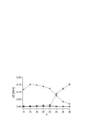
Figure 1: Comparison of the calculated HF energies in the SLy4 interaction among the HO, the KG and the hybrid basis-sets for the oxygen isotopes. The circles, pluses and crosses indicate the energies obtained from the HO, KG and hybrid sets, respectively. In all cases $K=7$. In each nucleus, the energy differences are measured from the lowest HF energy of those by the three basis-sets.

The variational character of the HF theory is available in comparing results among different basis-sets. As the total energy is lower, it is closer to the true HF energy, in principle. The total HF energies calculated with the HO, the KG and the hybrid basis-sets are shown in Fig. 1, where the energy differences from the lowest one is plotted for each nucleus. In comparison with the HO set, the KG set gives higher energies for the $A\leq 22$ oxygen isotopes, while in $A\geq 24$, where the neutron $1s_{1/2}$ orbit is occupied, the KG set gives lower energies than the HO set. This is ascribed to the broad radial distribution of the $1s_{1/2}$ orbit, which is hardly reproduced by the HO basis-set. The hybrid basis-set works very well in the whole region. The energies are close between the HO and the hybrid sets in ^14-22O, having the differences less than 0.01 MeV, and the hybrid set yields sizably lower energies than the KG set for all of the calculated oxygen isotopes. Thus the hybrid basis-set of Eq. (47) is adaptable both to stable and unstable nuclei.

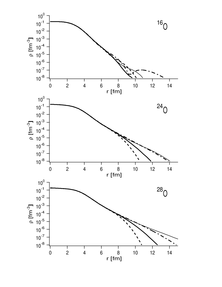
Figure 2: Comparison of the density distribution in the SLy4 interaction among the HO, KG and hybrid basis-sets for ¹⁶O, ²⁴O and ²⁸O. The dashed, dot-dashed and thick solid lines are obtained from the HO, KG and hybrid sets with $K=7$, respectively. As a reference, the densities obtained with the $K=15$ hybrid set are shown by the thin solid line.

In Fig. 2, the density distribution is compared among the three basis-sets, for ¹⁶O, ²⁴O and ²⁸O. The density distribution in $r>6$ fm tends to obey to the exponential asymptotics. Obviously, the density by the HO basis-set does not distribute sufficiently as $A$ increases, unable to reproduce the asymptotics for ²⁴O and ²⁸O. The densities in $r>6\,{\rm fm}$ calculated with the HO set behave quite analogously among the three nuclei, suggesting that they originate in the character of the bases and are not physical. Therefore the HO set is practically incapable of reproducing the asymptotics. On the contrary, the KG and the hybrid basis-sets reproduce the exponential asymptotics rather well. Although the KG set does not give the exact exponential asymptotics, it is possible to approximate the asymptotics by the KG set in an effective sense. The same holds for the hybrid set. If the density becomes extremely low, it is difficult to be reproduced by the KG set. For this reason, the KG set shows fictitious behavior of the density for $r>9$ fm in ¹⁶O, although the hybrid set yields rather smooth decrease. For ²⁴O and ²⁸O, the densities obtained by the KG set distribute more broadly than those by the hybrid set. This seems to caused by the difference in the longest range of the bases, on which it depends how slowly decreasing density can be described. Because we set the longest range to be $\nu_{\omega}\,b^{3}$ in the KG set while $\nu_{\omega}\,b^{2}$ in the hybrid one, the KG set can reproduce broader distribution that the hybrid set.

Figure 2 shows the high adaptability of the KG basis-set, particularly for the wave-functions in the asymptotic region. The energy-dependent asymptotics are reproduced reasonably well by a small number of bases. Unlike the HO basis, an individual basis in the KG set will not be a good first approximation of the nuclear s.p. wave-function. Nevertheless, when a certain number of bases are superposed, the KG set acquires remarkable flexibility in describing wave-functions. In the nuclear wave-functions, the exponent of the asymptotic form is energy dependent, as is viewed in the nucleus dependence in Fig. 2. The KG set (and therefore the hybrid set) well approximates the exponentially damping wave-functions with a moderate number of bases, whatever the separation energy is.

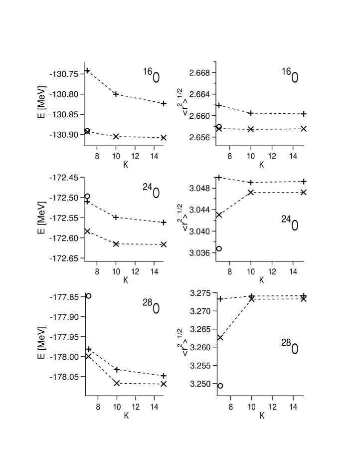
Figure 3: HF energies and rms matter radii of ¹⁶O, ²⁴O and ²⁸O in the SLy4 interaction, as a function of $K$ (i.e. number of the bases). The circles, pluses and crosses represent the results of the HO, KG and hybrid basis-sets, respectively. The dashed lines are drawn to guide eyes.

We next increase $K$, the number of the bases for each $\ell$ and $j$. The HF calculation is carried out using the KG and the hybrid basis-sets for $K=10$ and $15$. In the case of $K=10$, we take $\nu_{1}=\nu_{\omega}\,b^{-4}$ both for the KG and the hybrid sets, giving the longest range $\nu_{K}\cong 10\,{\rm fm}$ for the KG and $\nu_{K-1}\cong 7.5\,{\rm fm}$ for the hybrid set. In the calculation with $K=15$, we take $\nu_{1}=\nu_{\omega}\,b^{-5}$ for the KG set and $\nu_{\omega}\,b^{-4}$ for the hybrid set, both having the longest range of $31\,{\rm fm}$. In Fig. 3, the HF energies and the rms matter radii are plotted as a function of $K$, for ¹⁶O, ²⁴O and ²⁸O. The density distributions obtained by the hybrid set of $K=15$ are already shown in Fig. 2. For the matter radii, the center-of-mass correction is neglected, corresponding to the density distributions depicted in Fig. 2, in order to view the properties of the basis-sets directly. Owing to the variational character, the HF energies become lower as $K$ increases. If we adopt the KG set, the HF energies decrease slowly for increasing $K$. On the contrary, the HF energies by the hybrid basis-set are stable between $K=10$ and $15$, where the biggest decrease among ^14-28O is merely 0.003 MeV. This sort of stability is also viewed in the rms matter radii. Although the radii tend to be underestimated by the hybrid set with $K=7$, their difference between the $K=10$ and $15$ cases are negligibly small; less than $1.5\times 10^{-4}\,{\rm fm}$ for all the ^14-28O nuclei. By comparing with the $K=15$ hybrid basis-set, we view that the HO set provides reasonable values of the HF energies and the matter radii in the stable nucleus ¹⁶O, while it is not satisfactory in the unstable ones such as ²⁴O and ²⁸O.

Though one may think that the HF energies are convergent in the $K=15$ result using the hybrid basis-set, it does not imply the full convergence. The HF energies further decrease, if we use smaller $b$. Indeed, the HF energy becomes lower by about 0.01 MeV for a few of the oxygen isotopes, if we use $b=1.25$. As in the calculations so far, it is quite a laborious work to attain the full convergence in the HF calculation, and is beyond the scope of this article. In the same regard, the HF energies shown in Figs. 1 and 2 do not immediately mean a drawback of the KG set itself. It is only indicated that the KG set with $b=1.33$ is not sufficient to describe the nuclear wave-functions in the surface or the interior region. If we use smaller $b$ than the present value, the wave-functions around the surface may be reproduced more accurately, though it requires larger number of bases. It will be fair to say that the convergence is accelerated by using the hybrid set, compared with the case of the KG set.

In the present approach, the most time-consuming part in the numerical calculation is the computation of the two-body interaction matrix elements. It takes about 430 sec of CPU time on HITAC SR8000 to calculate all the necessary matrix elements up to the $sd$-shell when $K=7$, although the program has not yet been tuned. Moreover, the CPU time for computing the two-body matrix elements is almost proportional to $K^{4}$. On the other hand, the HF iteration need about 30 sec for each nucleus, and has dependence weaker than $K^{2}$. Under this situation, a great advantage of the KG basis-set is that it does not include parameters specific to mass number or nuclide. Hence the same basis-set can be used for a number of nuclei. With this advantage of the KG set, we have to calculate the two-body interaction matrix elements only once and do not have to recalculate them in systematic studies, and thereby we can save the computation time.

5.3 Case of finite-range interaction

The present method of the HF calculation can be used for finite-range interactions. We demonstrate it via the calculation with the Gogny D1S interaction.

There is a problem in the Gogny D1S force when it is applied to the mean-field calculations using the KG basis-set [7]. For the pure neutron matter with the D1S force, the energy per nucleon diverges with the negative sign at the high density limit. Originating in this defect, the HF energy goes to negative infinity in the finite nuclei, when all the neutrons gather in the vicinity of the origin (i.e. the center-of-mass) without overlap of the proton distribution. For the $\beta$-stable nuclei, this unphysical configuration is well separated from the normal HF solution, i.e. an energy minimum satisfying the saturation properties, and the normal solution is stable enough to be obtained in the numerical calculations. However, it is not the case for the highly neutron-rich nuclei. Even if the initial configuration is in the physical domain, the tunneling to the unphysical configuration takes place before convergence. In order to circumvent the tunneling, we need a certain cut-off of the high momentum components. In the previous studies [5], a sort of cut-off was implicitly introduced by adopting a limited number of the HO bases. On the other hand, we have to be cautious when we use the KG set. The wave-function of ²⁴O collapses via the tunneling when bases having $\nu_{\alpha}\leq 1\,{\rm fm}$ are included. Alternative to cutting off the high momentum components, a way to avoid this problem is to modify the interaction parameters, say, $x_{3}$ in $v_{12}^{\rm DD}$. This possibility will be explored in a forthcoming paper [7].

In the numerical calculations, we use the HO, the KG and the hybrid basis-sets of (44), (46) and (47). For the HO set, we take $K=7$ for each $\ell$ and $j$, assuming the same value of $\nu_{\omega}$ as in the preceding subsection. This corresponds to the $N_{\rm sh}\leq 13$ truncation except for the $d$-orbits, for which the $N_{\rm sh}=14$ bases are included, and this basis-set is similar to that used in most mean-field calculations with the Gogny interaction so far. For the KG and hybrid sets, we use $\nu_{1}=\nu_{\omega}\,b^{-2}$ and $b=1.33$, i.e. $\nu_{1}=1.36\,{\rm fm}$, and $K=12$.

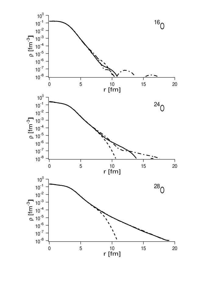
Figure 4: Comparison of the density distribution in the D1S interaction among the HO, KG and hybrid basis-sets for ¹⁶O, ²⁴O and ²⁸O. The dashed, dot-dashed and solid lines are obtained from the HO, KG and hybrid sets, respectively.

The density distributions of ¹⁶O, ²⁴O and ²⁸O are depicted in Fig. 4. The KG as well as the hybrid bases yield the reasonable asymptotics for unstable nuclei, whereas the HO set does not. The variational character is not fully available until establishing a rigorous cut-off scheme. However, it is still informative to compare the HF energies, as shown in Table 1. It is very likely that the energy of ²⁸O by the HO set is hampered by the ill asymptotic behavior, being higher than the energy of the KG set. As in the SLy4 case, the hybrid set gives the lowest energies in all of ¹⁶O, ²⁴O and ²⁸O. Thus the wave-functions in the asymptotic region, which have a sizable contribution to the physical quantities in highly neutron-rich nuclei, might not be described properly in the previous Gogny mean-field calculations by the HO bases, even though the $\nu_{\omega}$ parameter is better tuned than in the present calculation.

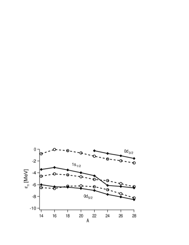
Figure 5: Neutron single-particle energies for the oxygen isotopes, obtained from the HF calculations with the SLy4 (open circles) and with the D1S (diamonds) interactions. The lines are drawn to guide eyes.

We next compare the HF results of the Gogny D1S interaction with those of the Skyrme SLy4 interaction. In Fig. 5, the neutron s.p. energies of the $sd$-shell orbits are shown for the oxygen isotopes. For ^14-20O, the $0d_{3/2}$ orbit is unbound in the D1S results, and hence its energies are not presented. The s.p. energies obtained from the SLy4 and the D1S interactions are relatively close to each other. A notable difference is found in the behavior of $\epsilon_{n}(1s_{1/2})$ around ²⁴O; the D1S interaction gives a kink at ²⁴O, while the SLy4 does not. When the $N$ (neutron number) dependence of the s.p. energies in ^16-22O is an effect of the occupation of $0d_{5/2}$, changes in the s.p. energies from ²²O to ²⁴O and from ²⁴O to ²⁸O are connected to the $1s_{1/2}$ and $0d_{3/2}$ occupation. It was argued based on the recent experimental data [20] that $N=16$ becomes a magic number in the neutron-rich region. The behavior of the s.p. energies around ²⁴O could be relevant to the magicity of $N=16$. The kink in the D1S result gives rise to the relatively large gap between $\epsilon_{n}(1s_{1/2})$ and $\epsilon_{n}(0d_{3/2})$ at ²⁴O. This would make the ²⁴O core stiffer than in the SLy4 interaction. We have confirmed that the kink viewed in the Gogny D1S result does not emerge in the results of other popular parameter-sets of the Skyrme interaction, as well as in the SLy4 result. Still it is not clear whether or not the range of the interaction plays a role in this kink. It is also commented that the kink at ²⁴O in the D1S interaction is not apparent when we use the HO basis-set, probably because of the wrong asymptotics.

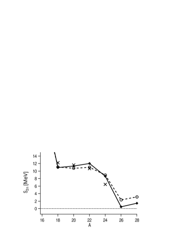
Figure 6: Two-neutron separation energies for the oxygen isotopes, obtained from the HF calculations with the SLy4 (open circles) and with the D1S (diamonds) interactions. The cross symbols represent the experimental data [21].

The two-neutron separation energy $S_{2n}$ is calculated as difference of the binding energies between the neighboring isotopes. The calculated values of $S_{2n}$ by the hybrid basis-set ($K=15$ for SLy4 and $K=12$ for D1S) are shown and compared with the measured ones [21] in Fig. 6. The $S_{2n}$ values are not very different between the SLy4 and D1S interactions for ^18-24O. It has been confirmed experimentally that ²⁶O and ²⁸O are unbound [22, 23]. This indicates $S_{2n}<0$ for ²⁶O. This feature is not reproduced in the SLy4 result. In the D1S interactions, we have slightly positive $S_{2n}$. However, this seems to depend somewhat on the details of the numerical set-ups; for example, the treatment of the center-of-mass correction. We just state that, in respect to $S_{2n}$ at ²⁶O, the D1S interaction gives preferable result to the SLy4 interaction.

In the present calculations we do not take into account sufficiently the collectivity due to the pairing correlations. If we rely on the shell closure at $N=16$, the pairing correlations will hardly change the energy of ²⁴O, while they lower the energies of ²²O and ²⁶O to a certain extent. Thus the pairing effects are expected to give lower $S_{2n}$ at ²⁴O and higher $S_{2n}$ at ²⁶O than the present HF values, if we perform a Hartree-Fock-Bogolyubov calculation.

Concerning the computation time, it is noted that the interaction dependence is weak in the present method. The CPU time for the Gogny interaction is almost the same as in the Skyrme interaction.

6 Summary and outlook

We have developed a new method of the Hartree-Fock calculations. This method has advantages in reproducing the slowly decreasing density distributions in unstable nuclei by a proper selection of bases, and in treating various interactions including finite-range ones.

The key point of the method is adoption of the Gaussian bases shown in Eq. (1). This covers the Kamimura-Gauss (KG) basis-set, as well as the basis-set equivalent to the harmonic-oscillator (HO) one, and may open wider variety. We have also discussed a way to calculate two-body interaction matrix elements, by applying the Fourier transformation. This is particularly suitable to the Gaussian bases because the numerical integration can be avoided to a great extent. Owing to this treatment of the interaction, we can easily switch from an effective interaction to another.

The present method has numerically been tested by using the Skyrme SLy4 and the Gogny D1S forces, as representatives of the zero- and the finite-range interactions. The calculations with the HO basis-set and with the KG basis-set are compared. It has been confirmed that the KG set efficiently describes wave-functions in the asymptotic region for the neutron-rich nucleus such as ²⁴O and ²⁸O. When we adopt the KG set, we do not have to change the bases from nucleus to nucleus, since they do not contain nucleus-dependent parameters like $\hbar\omega$. Hence the KG basis-set is expected to be powerful for systematic calculations. We have also shown a way to improve the convergence over the KG set. If we use a hybrid basis-set, in which a HO-type basis is added to the bases in the KG set, the HF energies often decrease substantially. The results on the s.p. energies and on $S_{2n}$ are also compared between the SLy4 and the D1S interactions, for the oxygen isotopes.

The present method provides us with a useful tool to investigate structure of the unstable nuclei, particularly with finite-range interactions. It will also be interesting to reconsider the effective interaction within the mean-field approaches. We can deal with various finite-range interaction, not only for the central part, and even with the Yukawa form. A research project in this line is under way.

While we have assumed the spherical symmetry in the discussions in this paper, it is straightforward to extend it to the deformed nuclei. The future plan includes the extension to the Hartree-Fock-Bogolyubov approach, and the combination with the complex-scaling method so as to handle the resonant single-particle orbits.

The authors are grateful to K. Katō and H. Kurasawa for helpful discussions. This work is supported in part as Grant-in-Aid for Scientific Research (C), No. 13640263, by the Ministry of Education, Culture, Sports, Science and Technology, Japan. Numerical calculations are performed on HITAC SR8000 at Information Processing Center, Chiba University.

Appendices

Appendix A Matrix elements of momentum-dependent part of Skyrme interaction

The central part of the Skyrme interaction is parameterized as

$$v_{12}^{\rm C} = t_{0}(1+x_{0}P_{\sigma})\delta({\mathbf{r}}_{12})+\frac{1}{2}t_{1}(1+x_{1}P_{\sigma})[\delta({\mathbf{r}}_{12}){\mathbf{p}}_{12}^{2}+{\mathbf{p}}_{12}^{2}\delta({\mathbf{r}}_{12})]$$ (48)

$$+\,t_{2}(1+x_{2}P_{\sigma}){\mathbf{p}}_{12}\cdot\delta({\mathbf{r}}_{12}){\mathbf{p}}_{12}\,.$$

As has been discussed in Section 4, the two-body matrix elements of the $t_{0}$ term can be treated in a unified way with the finite-range interactions. We here show that, though the $t_{1}$ and $t_{2}$ terms depend on the relative momentum ${\mathbf{p}}_{12}$, they can also be treated in a similar manner by using the Fourier transformation.

We first recall the identity

$$\left[{\mathbf{p}}_{12},\left[{\mathbf{p}}_{12},\delta({\mathbf{r}}_{12})\right]\right]=-\left(\nabla_{12}^{2}\,\delta({\mathbf{r}}_{12})\right)\,,$$ (49)

where $\nabla_{12}=(\nabla_{1}-\nabla_{2})/2$. By using the Fourier transform of the delta function, we obtain

$$\left[{\mathbf{p}}_{12},\left[{\mathbf{p}}_{12},\delta({\mathbf{r}}_{12})\right]\right]=[{\mathbf{p}}_{12}^{2}\delta({\mathbf{r}}_{12})+\delta({\mathbf{r}}_{12}){\mathbf{p}}_{12}^{2}]-2{\mathbf{p}}_{12}\cdot\delta({\mathbf{r}}_{12}){\mathbf{p}}_{12}={1\over{(2\pi)^{3}}}\int k^{2}e^{i{\mathbf{k}}\cdot{\mathbf{r}}_{12}}d^{3}k\,.$$ (50)

Owing to the delta function, $[{\mathbf{p}}_{12}^{2}\delta({\mathbf{r}}_{12})+\delta({\mathbf{r}}_{12}){\mathbf{p}}_{12}^{2}]$ vanishes when it operates on the spatially odd two-particle states. Similarly, $2{\mathbf{p}}_{12}\cdot\delta({\mathbf{r}}_{12}){\mathbf{p}}_{12}$ vanishes when acting on the spatially even states. Hence we can write

$$[{\mathbf{p}}_{12}^{2}\delta({\mathbf{r}}_{12})+\delta({\mathbf{r}}_{12}){\mathbf{p}}_{12}^{2}] = {1\over{(2\pi)^{3}}}\int k^{2}e^{i{\mathbf{k}}\cdot{\mathbf{r}}_{12}}d^{3}k\cdot(P_{\rm SE}+P_{\rm TE})\,,$$

$$-2{\mathbf{p}}_{12}\cdot\delta({\mathbf{r}}_{12}){\mathbf{p}}_{12} = {1\over{(2\pi)^{3}}}\int k^{2}e^{i{\mathbf{k}}\cdot{\mathbf{r}}_{12}}d^{3}k\cdot(P_{\rm SO}+P_{\rm TO})\,.$$ (51)

The projection operators $P_{\rm SE}$, $P_{\rm TE}$, $P_{\rm SO}$ and $P_{\rm TO}$ can be incorporated in the spin-isospin part, by using Eqs. (11,12). Then the spatial matrix elements of $[{\mathbf{p}}_{12}^{2}\delta({\mathbf{r}}_{12})+\delta({\mathbf{r}}_{12}){\mathbf{p}}_{12}^{2}]$ and $-2{\mathbf{p}}_{12}\cdot\delta({\mathbf{r}}_{12}){\mathbf{p}}_{12}$ are both evaluated by setting $\tilde{f}_{\delta^{\prime\prime}}^{\rm C}(k)=k^{2}$ in Eq. (35).

Appendix B Matrix elements of LS interaction

The LS interaction $v_{12}^{\rm LS}$ in Eq. (10) can be handled in a similar manner to the central force. We here consider the non-anti-symmetrized matrix elements of the LS force,

$$\langle(j^{\prime}_{1}j^{\prime}_{2})J|v_{12}^{\rm LS}|(j_{1}j_{2})J\rangle=\sum_{\mu}\langle(j^{\prime}_{1}j^{\prime}_{2})J|(t_{\mu}^{\rm LSE}P_{\rm TE}+t_{\mu}^{\rm LSO}P_{\rm TO})f_{\mu}^{\rm LS}(r_{12})\,{\mathbf{L}}_{12}\cdot({\mathbf{s}}_{1}+{\mathbf{s}}_{2})|(j_{1}j_{2})J\rangle\,.$$ (52)

The LS force operates only on the spin-triplet two-particle states. As in Appendix A, we separate $P_{\rm TE}$ and $P_{\rm TO}$, denoting the projection operators by ${\cal O}_{\sigma\tau}(=P_{\rm TE}\mbox{ or }P_{\rm TO})$ and their expectation values by $\langle{\cal O}_{\sigma\tau}\rangle_{S=1}$. It is noted that $f_{\mu}^{\rm LS}(r_{12})$ should not be the delta function, since $\delta({\mathbf{r}}_{12}){\mathbf{L}}_{12}=0$.

From the definition of Eq. (13), ${\mathbf{L}}_{12}$ is rewritten as

$${\mathbf{L}}_{12}={1\over 2}(\mbox{\boldmath$\ell$}_{1}+\mbox{\boldmath$\ell$}_{2}-{\mathbf{r}}_{1}\times{\mathbf{p}}_{2}-{\mathbf{r}}_{2}\times{\mathbf{p}}_{1})\,,$$ (53)

where $\mbox{\boldmath$\ell$}_{1}={\mathbf{r}}_{1}\times{\mathbf{p}}_{1}$ and $\mbox{\boldmath$\ell$}_{2}={\mathbf{r}}_{2}\times{\mathbf{p}}_{2}$. Since the $(\mbox{\boldmath$\ell$}_{1}+\mbox{\boldmath$\ell$}_{2})$ operator does not change the spatial part of the wave-functions, the matrix elements regarding $(\mbox{\boldmath$\ell$}_{1}+\mbox{\boldmath$\ell$}_{2})$ is handled in an analogous way to the central force,

$$\langle(j^{\prime}_{1}j^{\prime}_{2})J|f_{\mu}^{\rm LS}(r_{12})\,{1\over 2}(\mbox{\boldmath$\ell$}_{1}+\mbox{\boldmath$\ell$}_{2})\cdot({\mathbf{s}}_{1}+{\mathbf{s}}_{2}){\cal O}_{\sigma\tau}|(j_{1}j_{2})J\rangle\hskip 156.49014pt$$

$$=-\sum_{L}3(2L+1)\,{{J(J+1)-L(L+1)-2}\over 4}\sqrt{(2j_{1}+1)(2j_{2}+1)(2j^{\prime}_{1}+1)(2j^{\prime}_{2}+1)}$$

$$\times\left\{\begin{array}[]{ccc}l_{1}&{1\over 2}&j_{1}\\ l_{2}&{1\over 2}&j_{2}\\ L&1&J\end{array}\right\}\left\{\begin{array}[]{ccc}l^{\prime}_{1}&{1\over 2}&j^{\prime}_{1}\\ l^{\prime}_{2}&{1\over 2}&j^{\prime}_{2}\\ L&1&J\end{array}\right\}\langle(l^{\prime}_{1}l^{\prime}_{2})L|f_{\mu}^{\rm LS}(r_{12})|(l_{1}l_{2})L\rangle\,\langle{\cal O}_{\sigma\tau}\rangle_{S=1}\,.\quad$$ (60)

The $\langle(l^{\prime}_{1}l^{\prime}_{2})L|f_{\mu}^{\rm LS}(r_{12})|(l_{1}l_{2})L\rangle$ matrix elements are given in Eq. (35), except that $\tilde{f}_{\mu}^{\rm C}(k)$ is replaced by $\tilde{f}_{\mu}^{\rm LS}(k)$, the Fourier transform of $f_{\mu}^{\rm LS}(r_{12})$.

For the part including $({\mathbf{r}}_{1}\times{\mathbf{p}}_{2})$, we separate the spatial and the spin parts again, having

$$\langle(j^{\prime}_{1}j^{\prime}_{2})J|f_{\mu}^{\rm LS}(r_{12})\,{1\over 2}({\mathbf{r}}_{1}\times{\mathbf{p}}_{2})\cdot({\mathbf{s}}_{1}+{\mathbf{s}}_{2}){\cal O}_{\sigma\tau}|(j_{1}j_{2})J\rangle\hskip 156.49014pt$$

$$=-\sum_{L,L^{\prime}}3\sqrt{6(2L+1)(2L^{\prime}+1)(2j_{1}+1)(2j_{2}+1)(2j^{\prime}_{1}+1)(2j^{\prime}_{2}+1)}\,W(L\,J\,1\,1;1\,L^{\prime})$$

$$\times\left\{\begin{array}[]{ccc}l_{1}&{1\over 2}&j_{1}\\ l_{2}&{1\over 2}&j_{2}\\ L&1&J\end{array}\right\}\left\{\begin{array}[]{ccc}l^{\prime}_{1}&{1\over 2}&j^{\prime}_{1}\\ l^{\prime}_{2}&{1\over 2}&j^{\prime}_{2}\\ L^{\prime}&1&J\end{array}\right\}\langle(l^{\prime}_{1}l^{\prime}_{2})L^{\prime}||f_{\mu}^{\rm LS}(r_{12})\,{1\over 2}({\mathbf{r}}_{1}\times{\mathbf{p}}_{2})^{(1)}||(l_{1}l_{2})L\rangle\,$$ (67)

$$\times\langle{\cal O}_{\sigma\tau}\rangle_{S=1}\,,$$ (68)

As has been shown for the central part in Section 4, $f_{\mu}^{\rm LS}(r_{12})$ contains the angular part $[Y^{(\lambda)}(\hat{\mathbf{r}}_{1})\cdot Y^{(\lambda)}(\hat{\mathbf{r}}_{2})]$. Combining it with the $({\mathbf{r}}_{1}\times{\mathbf{p}}_{2})$ operator, we obtain

$$\left[Y^{(\lambda)}(\hat{\mathbf{r}}_{1})\cdot Y^{(\lambda)}(\hat{\mathbf{r}}_{2})\right]\,{1\over 2}({\mathbf{r}}_{1}\times{\mathbf{p}}_{2})^{(1)}=(-)^{\lambda+1}\sqrt{{2\lambda+1}\over 2}\,\left[Y^{(\lambda)}(\hat{\mathbf{r}}_{1})\,Y^{(\lambda)}(\hat{\mathbf{r}}_{2})\right]^{(0)}\,\left[r_{1}^{(1)}\nabla_{2}^{(1)}\right]^{(1)}$$

$$=(-)^{\lambda+1}\sum_{\lambda_{1},\lambda_{2}}\sqrt{{(2\lambda+1)(2\lambda_{2}+1)}\over 2}\,(\lambda\,0\,1\,0|\lambda_{1}\,0)\,W(1\,1\,\lambda_{1}\,\lambda;1\,\lambda_{2})\hskip 99.58464pt$$

$$\times r_{1}\left\{Y^{(\lambda_{1})}(\hat{\mathbf{r}}_{1})\left[Y^{(\lambda)}(\hat{\mathbf{r}}_{2})\nabla_{2}^{(1)}\right]^{(\lambda_{2})}\right\}^{(1)}\,.\quad$$ (69)

The Fourier transformation of Eq. (27) and the integration of the angular part yields

$$\langle(l^{\prime}_{1}l^{\prime}_{2})L^{\prime}||f_{\mu}^{\rm LS}(r_{12})\,{1\over 2}({\mathbf{r}}_{1}\times{\mathbf{p}}_{2})^{(1)}||(l_{1}l_{2})L\rangle\hskip 227.62204pt$$

$$=\sum_{\lambda_{1},\lambda_{2}}(-)^{\lambda_{2}}(2\lambda_{2}+1)\sqrt{{3(2\lambda_{1}+1)(2L+1)(2L^{\prime}+1)}\over 2}\,(\lambda\,0\,1\,0|\lambda_{1}\,0)\,W(1\,1\,\lambda_{1}\,\lambda;1\,\lambda_{2})\,$$

$$\times\left\{\begin{array}[]{ccc}l_{1}&l_{2}&L\\ \lambda_{1}&\lambda_{2}&1\\ l^{\prime}_{1}&l^{\prime}_{2}&L^{\prime}\end{array}\right\}\cdot\int_{0}^{\infty}k^{2}dk\,\tilde{f}_{\mu}^{\rm LS}(k)\sqrt{2l_{1}+1}\,(l_{1}\,0\,\lambda_{1}\,0|l^{\prime}_{1}\,0)\,{\cal I}_{1}^{(1)}(k)\hskip 28.45274pt$$ (73)

$$\times\left\{\sqrt{(l_{2}+1)(2l_{2}+3)}\,(l_{2}\!+\!1\,0\,\lambda\,0|l^{\prime}_{2}\,0)\,W(l_{2}\,1\,l^{\prime}_{2}\,\lambda;l_{2}\!+\!1\,\lambda_{2})\,{\cal I}_{2}^{(d+)}(k)\right.\hskip 42.67912pt$$

$$\left.-\sqrt{l_{2}(2l_{2}-1)}\,(l_{2}\!-\!1\,0\,\lambda\,0|l^{\prime}_{2}\,0)\,W(l_{2}\,1\,l^{\prime}_{2}\,\lambda;l_{2}\!-\!1\,\lambda_{2})\,{\cal I}_{2}^{(d-)}(k)\right\}\,,\hskip 42.67912pt$$ (74)

where

$${\cal I}_{i}^{(1)}(k) = \int_{0}^{\infty}r^{2}dr\,rj_{\lambda}(kr)R_{j^{\prime}_{i}}(r)R_{j_{i}}(r)\,,$$

$${\cal I}_{i}^{(d+)}(k) = \int_{0}^{\infty}r^{2}dr\,j_{\lambda}(kr)R_{j^{\prime}_{i}}(r)\left[\left({d\over{dr}}-{\ell_{i}\over r}\right)R_{j_{i}}(r)\right]\,,$$

$${\cal I}_{i}^{(d-)}(k) = \int_{0}^{\infty}r^{2}dr\,j_{\lambda}(kr)R_{j^{\prime}_{i}}(r)\left[\left({d\over{dr}}+{{\ell_{i}+1}\over r}\right)R_{j_{i}}(r)\right]\,.$$ (75)

The subscript $i$ to ${\cal I}$ corresponds to the nucleon index. The Gaussian bases of Eq. (1) give

$$\left({d\over{dr}}-{\ell\over r}\right)R_{\alpha\ell j}(r) = \left({{2p_{\alpha}}\over{r}}-{{2r}\over{\nu_{\alpha}^{2}}}\right)R_{\alpha\ell j}(r)\,,$$

$$\left({d\over{dr}}+{{\ell+1}\over r}\right)R_{\alpha\ell j}(r) = \left({{2\ell+2p_{\alpha}+1}\over{r}}-{{2r}\over{\nu_{\alpha}^{2}}}\right)R_{\alpha\ell j}(r)\,.$$ (76)

Hence the $r$ integration in Eq. (75) is implemented in a similar manner to Eq. (32). Because of the parity selection rule, the result is a product of a polynomial of $k$ and a Gaussian, and finally the $k$ integration has the form of Eq. (37). Thus the $k$ integration is carried out analytically for $f_{\mu}^{\rm LS}(r_{12})=e^{-(\mu r_{12})^{2}}$, while it is expressed by using the error function for $f_{\mu}^{\rm LS}(r_{12})=e^{-\mu r_{12}}/\mu r_{12}$. The matrix elements of the part coming from $({\mathbf{r}}_{2}\times{\mathbf{p}}_{1})$ in Eq. (53) are obtained by interchanging the nucleon indices 1 and 2, with an appropriate phase factor.

In the Skyrme and the Gogny interactions, the LS part is taken to be

$$v_{12}^{\rm LS}=2iW_{0}\left[{\mathbf{p}}_{12}\times\delta({\mathbf{r}}_{12}){\mathbf{p}}_{12}\right]\cdot({\mathbf{s}}_{1}+{\mathbf{s}}_{2})\,.$$ (77)

This type of the LS interaction is also treated in an analogous manner, by using the Fourier transformation. It is noted that this $v_{12}^{\rm LS}$ force operates only on the $S=1$, $T=1$ (i.e. spatially odd) channel, because of the $({\mathbf{s}}_{1}+{\mathbf{s}}_{2})$ operator and of $\delta({\mathbf{r}}_{12})$. Recall that

$$\delta({\mathbf{r}}_{12})=\lim_{\mu\rightarrow\infty}\left({\mu\over\sqrt{\pi}}\right)^{3}\,e^{-(\mu r_{12})^{2}}\,.$$ (78)

Substituting Eq. (78) into Eq. (77), we obtain

$$v_{12}^{\rm LS} = 2iW_{0}\lim_{\mu\rightarrow\infty}\left({\mu\over\sqrt{\pi}}\right)^{3}\left[{\mathbf{p}}_{12}\times e^{-(\mu r_{12})^{2}}{\mathbf{p}}_{12}\right]\cdot({\mathbf{s}}_{1}+{\mathbf{s}}_{2})$$ (79)

$$= -4W_{0}\left[\lim_{\mu\rightarrow\infty}{{\mu^{5}}\over{\pi^{3\over 2}}}e^{-(\mu r_{12})^{2}}\right]{\mathbf{L}}_{12}\cdot({\mathbf{s}}_{1}+{\mathbf{s}}_{2})\,.$$

We shall take the $\mu\rightarrow\infty$ limit after a certain algebra. By comparing Eq. (79) with Eq. (10), we can identify

$$f_{\delta^{\prime\prime}}^{\rm LS}(r_{12})=-4\lim_{\mu\rightarrow\infty}{{\mu^{5}}\over{\pi^{3\over 2}}}e^{-(\mu r_{12})^{2}}\,,$$ (80)

whose Fourier transform is

$$\tilde{f}_{\delta^{\prime\prime}}^{\rm LS}(k)=-4\lim_{\mu\rightarrow\infty}\mu^{2}\,e^{-(k/2\mu)^{2}}\,,$$ (81)

and $t_{\delta^{\prime\prime}}^{\rm LSO}=W_{0}$. We here use the suffix $\delta^{\prime\prime}$ to stand for the spatial part of the LS force (77), for the reason clarified in the discussion below. By expanding the exponential factor and taking the $\mu\rightarrow\infty$ limit except the non-vanishing terms, we have

$$\tilde{f}_{\delta^{\prime\prime}}^{\rm LS}(k)=-4\left(\lim_{\mu\rightarrow\infty}\mu^{2}\right)+k^{2}\,.$$ (82)

Although the first term in the right-hand side looks divergent, it is obvious that its inverse Fourier transform is proportional to $\delta({\mathbf{r}}_{12})$, which turns out to vanish because $\delta({\mathbf{r}}_{12})\,{\mathbf{L}}_{12}=0$. We now pose safely, for the LS force of Eq. (77),

$$\tilde{f}_{\delta^{\prime\prime}}^{\rm LS}(k)=k^{2}\,.$$ (83)

This is the same form as in the momentum-dependent term discussed in Appendix A. Equation (83) corresponds to the modification of Eq. (80) as

$$f_{\delta^{\prime\prime}}^{\rm LS}(r_{12})=-4\lim_{\mu\rightarrow\infty}\mu^{2}\left[\left({\mu\over\sqrt{\pi}}\right)^{3}\,e^{-(\mu r_{12})^{2}}-\delta({\mathbf{r}}_{12})\right]\,.$$ (84)

Thus the LS force in the Skyrme and Gogny interactions is treated in a unified way with the finite-range LS forces.

Appendix C Matrix elements of tensor interaction

We turn to the non-anti-symmetrized matrix elements of the tensor force,

$$\langle(j^{\prime}_{1}j^{\prime}_{2})J|v_{12}^{\rm TN}|(j_{1}j_{2})J\rangle=\sum_{\mu}\langle(j^{\prime}_{1}j^{\prime}_{2})J|(t_{\mu}^{\rm TNE}P_{\rm TE}+t_{\mu}^{\rm TNO}P_{\rm TO})f_{\mu}^{\rm TN}(r_{12})\,r_{12}^{2}S_{12}|(j_{1}j_{2})J\rangle\,.$$ (85)

The tensor force operates only on the spin-triplet two-particle states. As in Appendix B, we shall denote $P_{\rm TE}$ or $P_{\rm TO}$ by ${\cal O}_{\sigma\tau}$.

By separating the spatial degrees-of-freedom from the spin ones, the tensor operator of Eq. (14) is rewritten as

$$r_{12}^{2}S_{12}=8\left\{\sqrt{{6\pi}\over 5}\left[r_{1}^{2}Y^{(2)}(\hat{\mathbf{r}}_{1})+r_{2}^{2}Y^{(2)}(\hat{\mathbf{r}}_{2})\right]-4\pi r_{1}r_{2}\left[Y^{(1)}(\hat{\mathbf{r}}_{1})Y^{(1)}(\hat{\mathbf{r}}_{2})\right]^{(2)}\right\}\cdot\left[s_{1}^{(1)}s_{2}^{(1)}\right]^{(2)}\,.$$ (86)

The matrix element of the $r_{1}^{2}Y^{(2)}(\hat{\mathbf{r}}_{1})$ part is given by, after calculating the spin part,

$$\langle(j^{\prime}_{1}j^{\prime}_{2})J|f_{\mu}^{\rm TN}(r_{12})\cdot 8\sqrt{{6\pi}\over 5}\,r_{1}^{2}Y^{(2)}(\hat{\mathbf{r}}_{1})\cdot\left[s_{1}^{(1)}s_{2}^{(1)}\right]^{(2)}{\cal O}_{\sigma\tau}|(j_{1}j_{2})J\rangle\hskip 99.58464pt$$

$$=\sum_{L,L^{\prime}}12\sqrt{5(2L+1)(2L^{\prime}+1)(2j_{1}+1)(2j_{2}+1)(2j^{\prime}_{1}+1)(2j^{\prime}_{2}+1)}\,W(L\,J\,2\,1;1\,L^{\prime})$$

$$\times\left\{\begin{array}[]{ccc}l_{1}&{1\over 2}&j_{1}\\ l_{2}&{1\over 2}&j_{2}\\ L&1&J\end{array}\right\}\left\{\begin{array}[]{ccc}l^{\prime}_{1}&{1\over 2}&j^{\prime}_{1}\\ l^{\prime}_{2}&{1\over 2}&j^{\prime}_{2}\\ L^{\prime}&1&J\end{array}\right\}\langle(l^{\prime}_{1}l^{\prime}_{2})L^{\prime}||f_{\mu}^{\rm TN}(r_{12})\sqrt{{6\pi}\over 5}r_{1}^{2}Y^{(2)}(\hat{\mathbf{r}}_{1})||(l_{1}l_{2})L\rangle$$ (93)

$$\times\langle{\cal O}_{\sigma\tau}\rangle_{S=1}\,.\quad$$ (94)

By using the Fourier transform of $f_{\mu}^{\rm TN}(r_{12})$ and integrating out the angular part, we obtain for the spatial matrix element,

$$\langle(l^{\prime}_{1}l^{\prime}_{2})L^{\prime}||f_{\mu}^{\rm TN}(r_{12})\sqrt{{6\pi}\over 5}r_{1}^{2}Y^{(2)}(\hat{\mathbf{r}}_{1})||(l_{1}l_{2})L\rangle\hskip 199.16928pt$$

$$=(-)^{\lambda}\sum_{\lambda_{1}}\sqrt{{3(2\lambda_{1}+1)(2L+1)(2L^{\prime}+1)}\over 2}\,(\lambda\,0\,2\,0|\lambda_{1}\,0)\left\{\begin{array}[]{ccc}l_{1}&l_{2}&L\\ \lambda_{1}&\lambda&2\\ l^{\prime}_{1}&l^{\prime}_{2}&L^{\prime}\end{array}\right\}\hskip 56.9055pt$$ (98)

$$\times\int_{0}^{\infty}k^{2}dk\,\tilde{f}_{\mu}^{\rm TN}(k)\sqrt{2l_{1}+1}\,(l_{1}\,0\,\lambda_{1}\,0|l^{\prime}_{1}\,0)\,{\cal I}^{(2)}_{1}(k)\cdot\sqrt{2l_{2}+1}\,(l_{2}\,0\,\lambda\,0|l^{\prime}_{2}\,0)\,{\cal I}^{(0)}_{2}(k)\,,$$ (99)

where

$${\cal I}_{i}^{(2)}(k)=\int_{0}^{\infty}r^{2}dr\,r^{2}j_{\lambda}(kr)R_{j^{\prime}_{i}}(r)R_{j_{i}}(r)\,,$$ (100)

and ${\cal I}_{i}^{(0)}$ is defined in Eq. (31). The matrix element of the $r_{2}Y^{(2)}(\hat{\mathbf{r}}_{2})$ part in the expansion of Eq. (86) is obtained by an appropriate replacement between the nucleon indices.

After the algebra regarding the spin degrees-of-freedom, we have for the matrix elements of the $r_{1}r_{2}[Y^{(1)}(\hat{\mathbf{r}}_{1})Y^{(1)}(\hat{\mathbf{r}}_{2})]^{(2)}$ part,

$$\langle(j^{\prime}_{1}j^{\prime}_{2})J|f_{\mu}^{\rm TN}(r_{12})\cdot 8\cdot 4\pi\,r_{1}r_{2}\left[Y^{(1)}(\hat{\mathbf{r}}_{1})Y^{(1)}(\hat{\mathbf{r}}_{2})\right]^{(2)}\cdot\left[s_{1}^{(1)}s_{2}^{(1)}\right]^{(2)}{\cal O}_{\sigma\tau}|(j_{1}j_{2})J\rangle\hskip 42.67912pt$$

$$=\sum_{L,L^{\prime}}12\sqrt{5(2L+1)(2L^{\prime}+1)(2j_{1}+1)(2j_{2}+1)(2j^{\prime}_{1}+1)(2j^{\prime}_{2}+1)}\,W(L\,J\,2\,1;1\,L^{\prime})\hskip 28.45274pt$$

$$\times\left\{\begin{array}[]{ccc}l_{1}&{1\over 2}&j_{1}\\ l_{2}&{1\over 2}&j_{2}\\ L&1&J\end{array}\right\}\left\{\begin{array}[]{ccc}l^{\prime}_{1}&{1\over 2}&j^{\prime}_{1}\\ l^{\prime}_{2}&{1\over 2}&j^{\prime}_{2}\\ L^{\prime}&1&J\end{array}\right\}\langle(l^{\prime}_{1}l^{\prime}_{2})L^{\prime}||f_{\mu}^{\rm TN}(r_{12})\,4\pi r_{1}r_{2}\left[Y^{(1)}(\hat{\mathbf{r}}_{1})Y^{(1)}(\hat{\mathbf{r}}_{2})\right]^{(2)}||(l_{1}l_{2})L\rangle$$ (107)

$$\times\langle{\cal O}_{\sigma\tau}\rangle_{S=1}\,.\quad$$ (108)

For the spatial matrix elements, we obtain

$$\langle(l^{\prime}_{1}l^{\prime}_{2})L^{\prime}||f_{\mu}^{\rm TN}(r_{12})\,4\pi r_{1}r_{2}\left[Y^{(1)}(\hat{\mathbf{r}}_{1})Y^{(1)}(\hat{\mathbf{r}}_{2})\right]^{(2)}||(l_{1}l_{2})L\rangle\hskip 142.26378pt$$

$$=(-)^{\lambda}\sum_{\lambda_{1},\lambda_{2}}3\sqrt{5(2\lambda_{1}+1)(2\lambda_{2}+1)(2L+1)(2L^{\prime}+1)}\,(\lambda\,0\,1\,0|\lambda_{1}\,0)\,(\lambda\,0\,1\,0|\lambda_{2}\,0)\hskip 14.22636pt$$

$$\times W(2\,1\,\lambda_{1}\,\lambda;1\,\lambda_{2})\left\{\begin{array}[]{ccc}l_{1}&l_{2}&L\\ \lambda_{1}&\lambda_{2}&2\\ l^{\prime}_{1}&l^{\prime}_{2}&L^{\prime}\end{array}\right\}\int_{0}^{\infty}k^{2}dk\sqrt{2l_{1}+1}\,(l_{1}\,0\,\lambda_{1}\,0|l^{\prime}_{1}\,0)\,{\cal I}^{(1)}_{1}(k)$$ (112)

$$\times\sqrt{2l_{2}+1}\,(l_{2}\,0\,\lambda_{2}\,0|l^{\prime}_{2}\,0)\,{\cal I}^{(1)}_{2}(k)\,,$$ (113)

where ${\cal I}_{i}^{(1)}$ is given in Eq. (75).

In Ref. [15], a zero-range tensor interaction was proposed to cancel out a certain term of the LS current. By separating it into the spatially even and odd channels, we have

$$v_{12}^{\rm TN}=4t_{\delta^{\prime\prime\prime\prime}}^{\rm TNE}\left\{\left[3({\mathbf{s}}_{1}\cdot{\mathbf{p}}_{12})({\mathbf{s}}_{2}\cdot{\mathbf{p}}_{12})-({\mathbf{s}}_{1}\cdot{\mathbf{s}}_{2}){\mathbf{p}}_{12}^{2}\right]\delta({\mathbf{r}}_{12})\right.\hskip 71.13188pt$$

$$\left.+\delta({\mathbf{r}}_{12})\left[3({\mathbf{s}}_{1}\cdot{\mathbf{p}}_{12})({\mathbf{s}}_{2}\cdot{\mathbf{p}}_{12})-({\mathbf{s}}_{1}\cdot{\mathbf{s}}_{2}){\mathbf{p}}_{12}^{2}\right]\right\}P_{\rm TE}$$

$$-4\,t_{\delta^{\prime\prime\prime\prime}}^{\rm TNO}\left\{3({\mathbf{s}}_{1}\cdot{\mathbf{p}}_{12})\delta({\mathbf{r}}_{12})({\mathbf{s}}_{2}\cdot{\mathbf{p}}_{12})+3({\mathbf{s}}_{2}\cdot{\mathbf{p}}_{12})\delta({\mathbf{r}}_{12})({\mathbf{s}}_{1}\cdot{\mathbf{p}}_{12})\right.$$

$$\left.-2({\mathbf{s}}_{1}\cdot{\mathbf{s}}_{2})\left[{\mathbf{p}}_{12}\cdot\delta({\mathbf{r}}_{12}){\mathbf{p}}_{12}\right]\right\}P_{\rm TO}\,.$$ (114)

In Ref. [15] $t_{\delta^{\prime\prime\prime\prime}}^{\rm TNO}={3\over 8}t_{\delta^{\prime\prime\prime\prime}}^{\rm TNE}$. By using the expression of Eq. (78), we obtain

$$f_{\delta^{\prime\prime\prime\prime}}^{\rm TN}(r_{12})=\lim_{\mu\rightarrow\infty}{{4\mu^{7}}\over{\pi^{3\over 2}}}\,e^{-(\mu r_{12})^{2}}\,,$$ (115)

whose Fourier transform yields

$$\tilde{f}_{\delta^{\prime\prime\prime\prime}}^{\rm TN}(k)={k^{4}\over 8}\,,$$ (116)

after eliminating the vanishing terms. Thus this type of the tensor force is also treated in a unified way with the finite-range tensor force.

Table 1: Hartree-Fock energies (MeV) in the D1S interaction for ¹⁶O, ²⁴O and ²⁸O, using the HO, KG and hybrid basis-sets.

nuclide	HO	KG	hybrid
16O	$-136.849$	$-136.720$	$-136.952$
24O	$-179.477$	$-179.445$	$-179.815$
28O	$-181.397$	$-181.501$	$-181.770$

References

• [1] I. Tanihata, Nucl Phys. A 654 (1999) 235c.
• [2] D. Vautherin and D. M. Brink, Phys. Rev. C 5 (1972) 626.
• [3] J. W. Negele and D. Vautherin, Phys. Rev. C 5 (1972) 1472.
• [4] F. Hoffmann and H. Lenske, Phys. Rev. C 57 (1998) 2281.
• [5] J. DechargΓ© and D. Gogny, Phys. Rev. C 21 (1980) 1568.
• [6] J. F. Berger, M. Girod and D. Gogny, Comp. Phys. Comm. 63 (1991) 365.
• [7] M. Sato and H. Nakada, in preparation.
• [8] H. Nakada and T. Otsuka, Phys. Rev. C 49 (1994) 886.
• [9] M. Kamimura, Phys. Rev. A 38 (1988) 621.
• [10] H. Kameyama, M. Kamimura and Y. Fukushima, Phys. Rev. C 40 (1989) 974.
• [11] M. V. Stoitsov, W. Nazarewicz and S. Pittel, Phys. Rev. C 58 (1998) 2092; M. V. Stoitsov, J. Dobaczewski, P. Ring and S. Pittel, Phys. Rev. C 61 (2000) 034311.
• [12] P.-G. Reinhardt, Computational Nuclear Physics vol.Β 1, edited by K. Langanke, J. A. Maruhn and S. E. Koonin (Springer-Verlag, Berlin, 1991), p.Β 28.
• [13] A. L. Fetter and J. D. Walecka, Quantum Theory of Many-Particle Systems (McGraw-Hill, New York, 1971), p.Β 31.
• [14] K. Andō and H. Bandō, Prog. Theor. Phys. 66 (1981) 227; S. C. Pieper and V. R. Pandharipande, Phys. Rev. Lett. 70 (1993) 2541.
• [15] M. Beiner, H. Flocard, N. van Giai and P. Quentin, Nucl. Phys. A 238 (1975) 29.
• [16] R.-G. Reinhardt and H. Flocard, Nucl. Phys. A 584 (1995) 467.
• [17] H. Horie and K. Sasaki, Prog. Theor. Phys. 25 (1961) 475.
• [18] M. Anguiano, J. L. Egido and L. M. Robledo, Nucl. Phys. A 683 (2001) 227.
• [19] E. Chabanat, P. Bonche, P. Haensel, J. Meyer and R. Schaeffer, Nucl. Phys. A 627 (1997) 710; ibid 635 (1998) 231.
• [20] A. Ozawa, T. Kobayashi, T. Suzuki, K. Yoshida and I. Tanihata, Phys. Rev. Lett. 84 (2000) 5493.
• [21] R. B. Firestone et al., Table of Isotopes, 8th edition (John Wiley & Sons, New York, 1996).
• [22] D. Guillemaud-Mueller et al., Phys. Rev. C 41 (1990) 937; M. Fauerbach et al., Phys. Rev. C 53 (1996) 647.
• [23] H. Sakurai et al., Phys. Lett. B 448 (1999) 180.