Structure of Light Unstable Nuclei Studied with Antisymmetrized Molecular Dynamics

Abstract

Structures of light unstable nuclei, Li, Be, B, and C isotopes are systematically studied with a microscopic method of antisymmetrized molecular dynamics. The theoretical method is found to be very useful to study ground and excited states of various nuclei covering unstable nuclei. The calculations succeed to reproduce many experimental data for nuclear structures; energies, radii, magnetic dipole moments, electric quadrupole moments, transition strength. In the theoretical results it is found that various exotic phenomena in unstable nuclei such as molecular-like structures, neutron skin, and large deformations may appear in unstabel nuclei. We investigate the structure change with the increase of neutron number and with the increase of the excitation energies, and find the drastic changes between shell-model-like structures and clustering structures. The mechanism of clustering developments in unstable nuclei are discussed.

Contents

toc

I Introduction

Owing to the progress of the experimental technique, the information of the ground and excited states of unstable nuclei is increasing rapidly. There are various interesting subjects which are characteristics of unstable nuclei. Our aim is to systematically study the nuclear structures of light nuclei covering stable and unstable regions in order to understand the features of the nuclear many-body system. In the light nuclear region, ground-state properties have become known experimentally for the unstable nuclei up to the drip line. The experimental data give various kinds of information such as binding energies, radii, magnetic dipole moments, and electric quadrupole moments, and so on [1, 2, 3, 4, 5, 6, 7, 8, 9, 10, 11, 12, 13]. By the help of these experimental data, many interesting phenomena of the structures of the unstable nuclei have been suggested; neutron halo and skin structures, vanishing of the magic number, abnormal spin-parity of the ground state, clustering structures, large deformations in unstable nuclei.

In many of the theoretical studies for light nuclei, inert cores or clusters have been assumed. For example, three-body models have been applied to ¹¹Li by regarding it as a ⁹Li+$2n$ system and also applied to ⁶He as an $\alpha$+$2n$ system [14, 15, 16]. In these studies the neutron-halo structure has been theoretically investigated. In the studies of very light nuclei with $A\leq 10$ with extended cluster models in which $\alpha$ or $t$ cluster cores and surrounding nucleons are assumed [17, 18, 19], it is suggested that the clustering structure may appear also in unstable nuclei. However, they have not yet reached to the systematic investigations covering the wide region of nuclei, since it is difficult to apply these models to the study of general heavier unstable nuclei. For heavier unstable nuclei, systematic studies have been done by using other theoretical frameworks such as shell model approaches [20] and the methods of mean field theory [21, 22]. Some of them suggested new features such as large deformations and neutron skin structures. However the applicability of mean-filed approaches is not necessarily assured in light nuclei because of possible clustering structures.

It is already well known that clustering structures [23, 24, 25, 26, 27] appear in the ground states of ordinary light nuclei with $N\approx Z$ as seen in the $t+\alpha$ cluster structure of ⁷Li and in the $\alpha+\alpha$ cluster structure of ⁸Be, and in the ¹⁶O+$\alpha$ cluster structure of ²⁰Ne. Therefore, in light unstable nuclei one of the problems to be solved is the clustering structure. Is the clustering seen also in unstable nuclei ? If it is the case, what is the feature of the clusters. How does the developed clustering structure of stable nuclei change with the increase of the neutron number in a series of isotopes ? It is naturally expected that the clustering structures of unstable nuclei are found not only in the ground state but also in the excited states. Recent experimental data suggest that the clustering structure may appear in excited states of unstable nuclei. For example, many excited states of ¹²Be have been found with the experiments of the breakup reactions from ¹²Be to ⁶He+⁶He and ⁸He+⁴He channels [28]. In theoretical studies, many groups have suggested clustering structures in neutron-rich nuclei and tried to discuss the features of the clustering [17, 18, 19, 29, 30]. It is essential for the systematic studies of unstable nuclei to describe both clustering aspects and shell-model-like aspects in one theoretical framework which is applicable to general nuclei. We are interested in how the structure changes with the increase of the neutron number and the excitation energy.

Our aim is to make systematic investigations of the structures of the ground and excited states of unstable nuclei with a microscopic model which is free from such assumptions as the inert core or the existence of clusters. Remarking the development of clustering structure, we try to understand many characteristic phenomena seen in unstable nuclei. We discuss the mechanism of clustering developments of unstable nuclei.

In this paper, we adopt a theoretical method of antisymmetrized molecular dynamics(AMD). Ono et al. have developed the method of AMD for the study of nuclear reactions [31, 32, 33, 34, 35]. The framework of AMD has been extended by Kanada-En’yo (one of the author of this paper) et al., and has been applied to the studies of nuclear structures [29, 30, 36, 37, 38, 39]. From these studies AMD has already proved to be a very useful theoretical approach for investigating the structure of the ground and excited states of light nuclei. In the AMD framework, basis wave functions of the system are given by Slater determinants where the spatial part of each single-particle wave function is a Gaussian wave packet. One of the characteristics of AMD is the flexibility of the wave function which can represent various clustering structures and shell-model-like structures, which is because no inert cores and no clusters are assumed. Another characteristic point of AMD is the frictional cooling method which is adopted in the energy variation for obtaining the ground and excited states. In the case of the simplest version of the AMD [29, 30] in this paper, the energy variation is made after the parity projection but before the total-spin projection. With this simplest method, we can describe low-lying levels of the lowest bands with positive and negative parities. For the study of the excited states we adopt the AMD approach which users the variation after the spin-parity projection (VAP). VAP calculations in AMD framework have been already found to be advantageous for the study of the excited states of light nuclei [38, 39]. By the use of microscopic calculations with the obtained wave functions, we can easily acquire the theoretical values of energies, radii, magnetic dipole moments, electric quadrupole moments, and the transition strength of $E1$, $E2$, and $\beta$ which are useful quantities to deduce the informations of structures from the experimental data.

This paper is organized as follows. In the next section (Sec. II) we explain the formulation of AMD for the study of nuclear structure. The effective interactions are described in Sec. III. In Sec. IV we show the results and give discussions of the Li, Be, B, and C isotopes based on the calculations of the simplest version of AMD. The study with VAP calculations in the framework of AMD is reported in Sec. V, where we discuss the structure of the excited states of neutron-rich Be isotopes. In Sec. VI, we mention about the mechanism of clustering developments of Be isotopes. Finally we give the summary in Sec.VII.

II Formulation

The AMD (antisymmetrized molecular dynamics) is a theory which is applicable to the studies of the nuclear structure and the nuclear reaction. Here we only explain the AMD framework for the study of nuclear structures. As for the AMD theory for the study of nuclear reaction, the reader is referred to Ref.[32].

A AMD wave function

In AMD framework, the wave function of a system is written by a linear combination of AMD wave functions,

$$\Phi=c\Phi_{AMD}+c^{\prime}\Phi^{\prime}_{AMD}+\cdots.$$ (1)

An AMD wavefunction is a Slater determinant of Gaussian wave packets;

$$\Phi_{AMD}({\bf Z})=\frac{1}{\sqrt{A!}}{\cal A}\{\varphi_{1},\varphi_{2},\cdots,\varphi_{A}\},$$ (2)

$$\varphi_{i}=\phi_{{\bf X}_{i}}\chi_{i}\tau_{i}:\left\{\begin{array}[]{l}\phi_{{\bf X}_{i}}({\bf r}_{j})\propto\exp\left[-\nu\biggl{(}{\bf r}_{j}-\frac{{\bf X}_{i}}{\sqrt{\nu}}\biggr{)}^{2}\right],\\ \chi_{i}=\left(\begin{array}[]{l}{1\over 2}+\xi_{i}\\ {1\over 2}-\xi_{i}\end{array}\right),\end{array}\right.$$ (7)

where $\chi_{i}$ is the intrinsic spin function parameterized by $\xi_{i}$, and $\tau_{i}$ is the isospin function which is up(proton) or down(neutron). Thus an AMD wave function is parameterized by a set of complex parameters ${\bf Z}\equiv\{X_{ni},\xi_{i}\}\ (n=1\sim 3\ \hbox{and }i=1\sim A)$.

If we consider a parity eigenstate projected from a Slater determinant the total wave function consists of two Slater determinants,

$$\Phi({\bf Z})=(1\pm P)\Phi_{AMD}({\bf Z}),$$ (8)

where $P$ is a parity projection operator. In case of total angular momentum eigenstates the wave function of a system is represented by integral of rotated states,

$$\Phi({\bf Z})=P^{J}_{MK^{\prime}}\Phi_{AMD}({\bf Z})=\int d\Omega D^{J*}_{MK^{\prime}}(\Omega)R(\Omega)\Phi_{AMD}({\bf Z}),$$ (9)

The expectation values of operators by $\Phi({\bf Z})$ are numerically calculated by a summation over mesh points of the Euler angles $\Omega$.

In principle the total wave function can be a superposition of independent AMD wave functions. We can consider a superposition of spin parity projected AMD wave functions $P^{J\pm}_{MK^{\prime}}\Phi_{AMD}$’s,

$$\Phi({\bf Z},{\bf Z}^{\prime})=cP^{J\pm}_{MK^{\prime}}\Phi_{AMD}({\bf Z})+c^{\prime}P^{J\pm}_{MK^{\prime}}\Phi_{AMD}({\bf Z}^{\prime})+\cdots.$$ (10)

B Energy variation

We make variational calculations to find the state which minimizes the energy of the system;

$${\cal E}=\frac{\langle\Phi|H|\Phi\rangle}{\langle\Phi|\Phi\rangle}$$ (11)

by the method of frictional cooling. Concerning with the frictional cooling method in AMD, the reader is referred to papers [29, 36]. For the wave function $\Phi({\bf Z})$ parameterized by complex parameters ${\bf Z}$, the time development of the parameters is determined by the frictional cooling equations,

$$\frac{dX_{nk}}{dt} = (\lambda+i\mu)\frac{1}{i\hbar}\frac{\partial{\cal E}({\bf Z},{\bf Z}^{\prime})}{\partial X^{*}_{nk}}=(\lambda+i\mu)\frac{1}{i\hbar}\frac{\partial}{\partial X^{*}_{nk}}\frac{\langle\Phi({\bf Z})|H|\Phi({\bf Z})\rangle}{\langle\Phi({\bf Z})|\Phi({\bf Z})\rangle},\quad(n=1\sim 3\quad k=1\sim A)$$ (12)

$$\frac{d\xi_{k}}{dt} = (\lambda+i\mu)\frac{1}{i\hbar}\frac{\partial{\cal E}({\bf Z},{\bf Z}^{\prime})}{\partial\xi^{*}_{k}}=(\lambda+i\mu)\frac{1}{i\hbar}\frac{\partial}{\partial\xi^{*}_{k}}\frac{\langle\Phi({\bf Z})|H|\Phi({\bf Z})\rangle}{\langle\Phi({\bf Z})|\Phi({\bf Z})\rangle},\quad(k=1\sim A)$$ (13)

with arbitrary real numbers $\lambda$ and $\mu<0$. It is easily proved that the energy of the system decreases with time as follows,

$$\frac{d{\cal E}}{dt} = \sum^{A}_{i=1}\left(\frac{\partial{\cal E}}{\partial{\bf X}_{i}}\cdot\frac{d{\bf X}_{i}}{dt}+\frac{\partial{\cal E}}{\partial{\bf X}^{*}_{i}}\cdot\frac{d{\bf X}^{*}_{i}}{dt}+\frac{\partial{\cal E}}{\partial\xi_{i}}\cdot\frac{d\xi_{i}}{dt}+\frac{\partial{\cal E}}{\partial\xi^{*}_{i}}\cdot\frac{d\xi^{*}_{i}}{dt}\right)$$ (14)

$$= \frac{2\mu}{\hbar}\sum^{A}_{i=1}\left(\frac{\partial{\cal E}}{\partial{\bf X}_{i}}\cdot\frac{\partial{\cal E}}{\partial{\bf X}^{*}_{i}}+\frac{\partial\cal E}{\partial\xi_{i}}\cdot\frac{\partial\cal E}{\partial\xi^{*}_{i}}\right)<0.$$ (15)

After sufficient time steps for cooling, the wave function of the minimum-energy state is obtained.

C Angular momentum projection

Expectation values of a given tensor operator $T^{k}_{q}$(rank $k$) for the total-angular-momentum projected states are written as follows,

$$\langle P^{J_{1}}_{M_{1}K_{1}}\Phi_{1}|T^{k}_{q}|P^{J_{2}}_{M_{2}K_{2}}\Phi_{2}\rangle$$ (16)

$$=\frac{2J_{2}+1}{8\pi^{2}}(J_{2}M_{2}kq|J_{1}M_{1})\sum_{K\nu}(J_{2}Kk\nu|J_{1}K_{1})\int d\Omega D^{J_{2}*}_{KK_{2}}(\Omega)\langle\Phi_{1}|T^{k}_{\nu}R(\Omega)|\Phi_{2}\rangle,$$ (17)

where $D^{J}_{MK}$ are the well-known Wigner’s D functions and $R(\Omega)$ stands for the rotation operator with Euler angles $\Omega$. In the practical calculations, the three-dimensional integral is evaluated numerically by taking a finite number of mesh points of the Euler angles $\Omega$.

D Simplest version of AMD for the study of nuclear structure

In the simplest version of AMD for the study of nuclear structure, the ground state wave function of a system is constructed by the energy variation of the parity eigenstate projected from a Slater determinant. Furthermore, the directions of intrinsic spins of single particle wave function are fixed to be up and down as $\xi_{i}=\pm\frac{1}{2}$ for simplicity. Therefore the spin-isospin functions of single-particle wave function are chosen as $p\uparrow$, $p\downarrow$, $n\uparrow$, and $n\downarrow$ in the initial state and are fixed in the energy variation. In this case the total wave function of a system is parameterized only by ${\bf X}\equiv\{{\bf X}_{1},{\bf X}_{2},\cdots,{\bf X}_{A}\}$ which are the centroids of Gaussian wave packets in the phase space,

$$\Phi({\bf X})=(1\pm P)\Phi_{AMD}({\bf X}).$$ (18)

We regard the minimum-energy state obtained with the energy variation (described in II B) for the parity projected state as the intrinsic state of the system. In order to compare with experimental data, we project the intrinsic wave function to the total-angular-momentum eigenstates and calculate the expectation values of operators. In that sense, “the simplest version of AMD” stands for the variational calculations after the parity projection but variation before projection (VBP) with respect to the total-angular momentum in this paper. In the same way as the ground state, the lowest non-normal parity state is calculated by energy variation for the non-normal parity projected state.

E Variation after projection

The wave function of the system should be a total-angular-momentum eigenstates. We can perform energy variation after the spin-parity projection(VAP) with the method of frictional cooling for the trial function $\Phi=P^{J\pm}_{MK^{\prime}}\Phi_{AMD({\bf Z})}$ [38].

First we make VBP calculation to prepare an initial state $\Phi_{AMD}({\bf Z}_{init})$ for the VAP calculation. We choose an appropriate $K^{\prime}$ quantum number for each spin parity that makes the energy expectation value for the spin parity eigenstate $\langle P^{J\pm}_{MK^{\prime}}\Phi_{AMD}({\bf Z}_{init})|H|P^{J\pm}_{MK^{\prime}}\Phi_{AMD}({\bf Z}_{init})\rangle/\langle P^{J\pm}_{MK^{\prime}}({\bf Z}_{init})|P^{J\pm}_{MK^{\prime}}({\bf Z}_{init})\rangle$ minimum. $K^{\prime}$ is a component of the total angular momentum along the approximately principal axis on the intrinsic system. In order to obtain the wave function for the lowest $J^{\pm}$ state, we perform VAP calculation for $\langle P^{J\pm}_{MK^{\prime}}\Phi_{AMD}({\bf Z})|H|P^{J\pm}_{MK^{\prime}}\Phi_{AMD}({\bf Z})\rangle/\langle P^{J\pm}_{MK^{\prime}}\Phi_{AMD}({\bf Z})|P^{J\pm}_{MK^{\prime}}\Phi_{AMD}({\bf Z})\rangle$ with the appropriate $K^{\prime}$ quantum number chosen for the initial state. In the VAP procedure, the principal $z$-axis of the intrinsic deformation is not assumed to equal with the $3$-axis of Euler angle in the total angular momentum projection. In general the principal $z$-axis is automatically determined in the energy variation. That is to say, the spin parity eigenstate $P^{J\pm}_{MK^{\prime}}\Phi_{AMD}$ obtained by VAP with a given $K^{\prime}=\langle J_{3}\rangle$ can be the state with so-called $K=\langle J_{z}\rangle$ quantum number mixing in terms of the intrinsic deformation.

F Higher excited states

As mentioned above, with the VAP calculation for $\Phi({\bf Z})=P^{J\pm}_{MK^{\prime}}\Phi_{AMD}({\bf Z})$ of the $J^{\pm}$ eigenstate with $K^{\prime}$ we obtain the wave function for the lowest $J^{\pm}$ state, which is represented by the set of parameters ${\bf Z}={\bf Z}^{J\pm}_{1}$. To search the parameters for the higher excited $J^{\pm}_{n}$ states, the wave functions are superposed so as to be orthogonal to the lower states as follows. The parameters ${\bf Z}^{J\pm}_{n}$ for the $n$-th $J^{\pm}$ state are reached by varying the energy of the orthogonal component to the lower states;

$$\Phi({\bf Z})=P^{J\pm}_{MK^{\prime}}\Phi_{AMD}({\bf Z})-\sum^{n-1}_{k=1}{\langle P^{J\pm}_{MK^{\prime}}\Phi_{AMD}({\bf Z}^{J\pm}_{k})|P^{J\pm}_{MK^{\prime}}\Phi_{AMD}({\bf Z})\rangle\over\langle P^{J\pm}_{MK^{\prime}}\Phi_{AMD}({\bf Z}^{J\pm}_{k})|P^{J\pm}_{MK^{\prime}}\Phi_{AMD}({\bf Z}^{J\pm}_{k})\rangle}P^{J\pm}_{MK^{\prime}}\Phi_{AMD}({\bf Z}^{J\pm}_{k}).$$ (19)

In the present paper, we call the variational calculation after the spin parity projection (mentioned in previous subsection) and the calculation for the higher excited states described in this subsection as VAP calculations.

G Diagonalization in VAP

After VAP calculations for various $J^{\pm}_{n}$ states mentioned above, the intrinsic states $\Phi^{1}_{AMD},\Phi^{2}_{AMD},\cdots,\Phi^{m}_{AMD}$, which correspond to the $J^{\pm}_{n}$ states, are obtained as much as the number of the calculated levels. Finally we construct the improved wave functions for the $J^{\pm}_{n}$ states by diagonalizing the Hamiltonian matrix $\langle P^{J\pm}_{MK^{\prime}}\Phi^{i}_{AMD}|H|P^{J\pm}_{MK^{\prime\prime}}\Phi^{j}_{AMD}\rangle$ and the norm matrix $\langle P^{J\pm}_{MK^{\prime}}\Phi^{i}_{AMD}|P^{J\pm}_{MK^{\prime\prime}}\Phi^{j}_{AMD}\rangle$ simultaneously with regard to ($i,j$) for all the intrinsic states and ($K^{\prime},K^{\prime\prime}$). In comparison with the experimental data such as energy levels and $E2$ transitions, the theoretical values are calculated with the final states after diagonalization.

III Interaction

For the effective two-nucleon interaction, we adopt the Volkov No.1 force [40] as the central force. The adopted parameters in this paper contain only Wigner and Majorana components. For some nuclei we have performed calculations by adding appropriate Bartlett and Heisenberg components to the Volkov force. However the results have proved to be not so much affected by the additional components except for the binding energies. Instead of the Volkov force, we also adopt case (1) and case (3) of MV1 force [41], which contain the zero-range three-body force $V^{(3)}$ as density dependent terms in addition to the two-body interaction $V^{(2)}$,

$$V_{DD} = V^{(2)}+V^{(3)}$$ (20)

$$V^{(2)} = (1-m+bP_{\sigma}-hP_{\tau}-mP_{\sigma}P_{\tau})\left\{V_{A}\exp\left[-\left(\frac{r}{r_{A}}\right)^{2}\right]+V_{R}\exp\left[-\left(\frac{r}{r_{R}}\right)^{2}\right]\right\},$$ (24)

$$b=h=0,$$

$$V_{A}=-83.34\hbox{MeV},r_{A}=1.60\hbox{fm},$$

$$V_{R}=104.86\hbox{MeV (case 1)},\qquad 99.86\hbox{MeV (case 3)},r_{R}=0.82\hbox{fm},$$

$$V^{(3)} = v^{(3)}\delta({\bf r}_{1}-{\bf r}_{2})\delta({\bf r}_{1}-{\bf r}_{3}),$$ (26)

$$v^{(3)}=4000\hbox{MeV fm${}^{6}$ for (case 1)},\qquad 5000\hbox{MeV fm${}^{6}$ (case 3)},$$

where $P_{\sigma}$ and $P_{\tau}$ stand for spin and isospin exchange operators, respectively, and $r$ denotes $|{\bf r}|\equiv|{\bf r}_{1}-{\bf r}_{2}|$. As for the two-body spin-orbit force $V_{LS}$, we adopt the G3RS force [42] ;

$$V_{LS}=\left\{u_{I}\exp\left(-\kappa_{I}r^{2}\right)+u_{II}\exp\left(-\kappa_{II}r^{2}\right)\right\}P(^{3}O){\bf L}\cdot({\bf S_{1}}+{\bf S_{2}}),$$ (27)

$${\bf L}\equiv{\bf r}\times\left(-i\frac{\partial}{\partial{\bf r}}\right),\qquad\kappa_{I}=5.0\hbox{fm}^{-2},\kappa_{II}=2.778\hbox{fm}^{-2},$$ (28)

with $P(^{3}O)$ denoting the projection operator onto the triplet odd$(^{3}O)$ two-nucleon state. The Coulomb interaction is approximated by a sum of seven Gaussians.

IV Study with simplest version of AMD

Since the wave function should be a total-angular-momentum eigenstate, it is expected that the VAP calculation gives better results than the simplest version of AMD. It is, however, not easy to perform VAP calculation because of the three-dimensional integral for the total-spin projection which is evaluated by taking a large number of mesh points of the Euler angles. In order to study systematically the structures of ground states of light nuclei covering from the ordinary region to the exotic unstable region, we perform the simplest version of AMD calculations (energy variation for the parity projected state) for even-odd, odd-even and even-even isotopes of Li, Be, B and C. The obtained states are projected to the total-angular-momentum eigenstates in calculating the expectation values to compare the results with the experimental data. Fortunately, in many nuclei with some exceptions, the obtained structures are not so much different from the ones obtained with VAP calculations. The results with VAP will be shown in the next section.

A Results

In this section the theoretical results of the simplest version of AMD are compared with the experimental data.

We have used the Volkov force with Majorana parameter $m=0.56$ ((a)), and the case 1 of MV1 force with $m=0.576$ ((b)) for the Li and Be isotopes. We have also adopted the MV1 force with mass dependent $m$ parameters ((c)) for B isotopes, and the MV1 force with $m=0.63$ ((d)). The adopted parameters are listed in Table II and II. The details are explained in each place. The optimum width parameters $\nu$ are shown in Table III, IV,V. The expectation values for the operators of observable quantities are calculated by projecting the intrinsic states obtained with the simplest version of AMD into the eigenstates of parity and total-angular-momentum. Most theoretical values except for the energy levels are obtained without the mixing of $K$-quantum which is the component of the spin $J$ along the approximate principal axis of the intrinsic system. Instead, we choose an appropriate $K$ which gives the minimum energy for each spin of a system. We have diagonalized the Hamiltonian matrix with respect to the $K$ quantum number within the spin $J$ projected states to calculate energy levels, and found only small mixing of the $K$ quantum number which implies that $K$ is approximately a good quantum number in the lowest $J^{\pm}$ states projected from the intrinsic states.

TABLE I.: The adopted interaction parameters.

(a)	Volkov No.1	$m=0.56$, $b=h=0$	$u_{I}=-u_{II}=900$ MeV
(b)	MV1 case(1)	$m=0.576$, $b=h=0$	$u_{I}=-u_{II}=900$ MeV
(d)	MV1 case(1)	$m=0.63$, $b=h=0$	$u_{I}=-u_{II}=900$ MeV
(e)	MV1 case(1)	$m=0.336$, $b=-0.2$, $h=0.4$	$u_{I}=-u_{II}=1500$ MeV

TABLE II.: The mass dependent interaction parameters of the force (c) adopted for B isotopes .

11B, 13B	MV1 case(1)	$m=0.576$, $b=h=0$	$u_{I}=-u_{II}=900$ MeV
15B	MV1 case(1)	$m=0.63$, $b=h=0$	$u_{I}=-u_{II}=900$ MeV
17B, 19B	MV1 case(1)	$m=0.65$, $b=h=0$	$u_{I}=-u_{II}=900$ MeV

TABLE III.: The width parameters $\nu$ of Gaussian wave packets adopted in the calculations of the simplest version of AMD for Li and Be isotopes. The optimum width parameter is chosen for each nucleus and each set of interactions.

		width parameter $\nu$ (fm-2)
	interaction	(a)	(b)
	6Be$(+)$	0.215	0.195
	7Be$(-)$	0.230	0.200
	8Be$(+)$	0.250	0.205
	9Be$(-)$	0.245	0.195
	9Be$(+)$	0.235	0.200
	10Be$(+)$	0.230	0.190
	10Be$(-)$	0.225	0.190
	11Be$(-)$	0.220	0.180
	11Be$(+)$	0.220	0.180
	12Be$(+)$	0.215	0.175
	12Be$(-)$	0.210	0.180
	13Be$(+)$	0.205	0.170
	14Be$(+)$	0.210	0.170
	7Li$(-)$	0.230	0.200
	9Li$(+)$	0.210	0.180
	11Li$(+)$	0.195	0.170

TABLE IV.: The optimum width parameters $\nu$ of Gaussian wave packets adopted for B isotopes.

	Width parameter $\nu$ (fm-2)
Interaction	11B	13B	15B	17B	19B
$m$=0.576	0.185	0.175	0.175	0.165	0.160
$m$=0.63	0.170	0.160	0.155	0.150	0.145
$m$=0.65	$-$	0.155	0.150	0.150	0.135

TABLE V.: The optimum width parameters $\nu$ of Gaussian wave packets adopted for C isotopes.

		width parameter $\nu$ (fm-2)
	interaction	(b)	(d)
	9C$(-)$	0.18	0.170
	10C$(+)$	0.19	0.180
	11C$(-)$	0.19	0.175
	12C$(+)$	0.19	0.175
	13C$(-)$	0.18	0.170
	14C$(+)$	0.18	0.165
	15C$(+)$	0.17	0.160
	16C$(+)$	0.17	0.160
	17C$(+)$	0.17	0.155
	18C$(+)$	0.17	0.150
	19C$(+)$	0.16	0.150
	20C$(+)$	0.16	0.145
	22C$(+)$	0.16	0.140

1 Energies

Figure 1 shows the binding energies of the ground states of Li and Be isotopes. With both of the interactions (a) and (b), the binding energies of Li and Be isotopes are qualitatively reproduced. The calculated result of ¹¹Be is the binding energy of the lowest $\frac{1}{2}^{+}$ state, though the normal-parity $\frac{1}{2}^{-}$ state is lower than $\frac{1}{2}^{+}$ state in these calculations. Detailed discussion of the energy levels and the parity of the ground state of ¹¹Be will be given later.

FIG. 1.: The binding energies of Li and Be isotopes. The circles(triangles) are the theoretical values with the interaction (a) ((b)). The square points indicate the experimental data.

FIG. 2.: The binding energies of B isotopes. The circles are the theoretical values calculated with the MV1 force with $m=0.576$, $0.63$, and $0.65$. The square points indicate the experimental data.

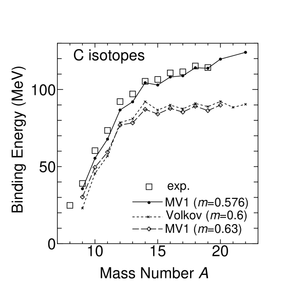
FIG. 3.: The binding energies of C isotopes. The lines are the theoretical values calculated with the MV1 force with $m=0.576$ and $0.63$. The figure also shows the calculations with the Volkov No.1 force with $m=0.6$. The square points indicate the experimental data.

The binding energies of B and C isotopes are presented in Fig.2 and Fig.3, respectively. For B isotopes, the figure shows theoretical results with the MV1 force with $m=0.576$, $m=0.63$, and $m=0.65$. In Fig. 3, results of C isotopes with Volkov($m=0.60$) and MV1 force with $m=0.576$ and $m=0.63$ are shown. For ¹⁵C the energies of $5/2^{+}$ states are shown, although the ground state should be $1/2^{+}$. In both B and C isotopes, MV1 force with $m=0.576$ reproduces well the experimental data.

FIG. 4.: The energy levels of Li and Be isotopes. The calculations with the interaction (a) Volkov No.1 force ($m=0.56$) and (b) MV1 force ($m=0.576$) are compared with the experimental data.

FIG. 5.: The energy levels of B isotopes. The adopted interactions are the case (b) MV1 force ($m=0.576$). The results for ¹¹B with the MV1 ($m=0.56$) and the spin-orbit force ($u_{I}=-u_{II}$=1500MeV) are also shown (f).

FIG. 6.: The energy levels of C isotopes. The theoretical values are obtained with the Volkov force ($m=0.6$) (f) and with the interaction (b) MV1 force ($m=0.576$). For the positive parity states of ¹³C and ¹⁵C, the results with the interaction (e) are presented instead of the ones with the interaction (b).

FIG. 7.: The energy levels of C isotopes. (See the figure caption in Fig.6)

The energy levels of Li, Be, B, and C isotopes are displayed in Fig.4, Fig.5, Fig.6, and Fig.7. The adopted interactions are explained in the figure captions. The second $J^{\pm}$ states are obtained by diagonalizing Hamiltonian with respect to $K$ quantum numbers. In many nuclei, the theoretical values of rotational bands such as excitation energies and spin sequence in low energy region well correspond to the experimental data. It means that many low-lying levels are approximately described as the rotated states of the intrinsic states obtained by the simplest AMD calculations which are VAP for parity projection but VBP for total-spin projection in the framework of AMD. Comparing the level spacing calculated with and without the three-body force, it is found that the states obtained with the three-body force have smaller level spacing, that is, larger moment of inertia. In many cases we found that the VBP calculation gives smaller level spacing than the VAP calculation.

The energy levels depend on the parameter $m$ of the Majorana exchange term and the presence of the three-body force. In general the results without the three-body force overestimate the excitation energies of non-normal parity states in most nuclei. The differences of the excitation energies between the normal parity and the non-normal parity states are improved in the results with the three-body force. In general the non-normal parity states have wider extension of the density distribution and therefore they feel relatively weaker repulsive force due to the three-body terms. It is the reason why the calculations with the three-body force give smaller excitation energies for the non-normal parity states. Even in the results with the three-body force, however, the non-normal parity $1/2^{+}$ state is still higher than the $1/2^{-}$ states in ¹¹Be which has been known to have abnormal parity of the ground state $1/2^{+}$. Careful choice of interactions and the improvement of the wave function is necessary to reproduce this feature of the parity inversion. For instance, VAP calculations with appropriate interaction parameters succeed to obtain the lower energy of $1/2^{+}$ state than the one of $1/2^{-}$ state. The detail will be mentioned later.

The energy levels of odd-even and even-odd nuclei are also sensitive to the strength of the spin-orbit force. The other set of interaction parameters (f) explained in the figure caption of Fig.5 give rather good results for energy levels of ¹¹B.

In ¹³C and ¹⁵C the lowest positive parity states are known to be $1/2^{+}$ states. However, the calculated intrinsic states of positive parity with MV1($m=0.576$) and Volkov force($m=0.60$) contain little component of $1/2^{+}$ states. Adopting other interaction parameter (e) in Table II: MV1 force with $m=0.336$, Bartlett and Heisenberg components $b=-0.2$, $h=0.4$ and the slightly stronger spin-orbit force with the magnitude of $u_{I}=-u_{II}=1500$MeV, we obtained the $1/2^{+}$ component whose energy is still rather higher than the one of $5/2^{+}$ state. In the result with every interaction, the main component of the intrinsic state obtained with VBP calculation is $5/2^{+}$, therefore, the variation affects to minimize the energy of $5/2^{+}$ state. For the lowest $1/2^{+}$ states of ¹³C and ¹⁵C, variations after spin-parity projection are useful instead of VBP calculations.

2 Radii

Figure 8 shows the radii of Li and Be isotopes. Dashed lines are the theoretical root-mean-square radii by AMD with the three-body force and dotted lines show results without three-body force. Square points indicate the experimental radii reduced from the experimental data of the interaction cross section. The AMD calculations with the three-body force seem to qualitatively agree with the observed radii except for the very neutron-rich nuclei. The theory underestimates the extremely large radii of ¹¹Li, ¹¹Be and ¹⁴Be which are considered to have the neutron halo structures. For reproduction of such large radii due to the halo structures, improvement of the wave function and careful choice of interactions should be important. The radius of the positive parity state of ¹²Be calculated with the present simple AMD calculation is smaller than the experimental datum because the obtained state has the closed neutron-$p$-shell structure. However VAP calculation with a set of interaction parameters which reproduces the parity inversion of the ¹¹Be ground state gives a ground state of ¹²Be as $2\hbar\omega$ state with 2 particles in $sd$ shell and 2 holes in $p$ shell in neutron configuration, whose radius is as large as the experimental data.

FIG. 8.: The root-mean-square radii of Li and Be isotopes. The solid lines and the dotted lines are the AMD results calculated with the interaction (a) Volkov force with $m=0.56$, and (b) MV1 force with $m=0.576$. The square points indicate the experimental data deduced from the interaction cross sections [5].

FIG. 9.: The root-mean-square radii of B isotopes. The triangles connected with the dotted line indicate the AMD results by the use of interaction (b) the fixed Majorana parameter $m=0.576$. The solid line shows the results by the interaction (c) with a mass-dependent Majorana parameter. The square points indicate the experimental data deduced from the interaction cross sections [5].

In Fig. 9, theoretical radii of B isotopes are compared with the experimental interaction radii. The triangles connected with the dotted line indicate the AMD results by the use of the fixed Majorana parameter $m=0.576$ (interaction(b)). The solid line shows the results by the interaction (c) with a mass-dependent Majorana parameter; $m=$0.576, 0.576, 0.63, 0.65, and 0.65 for ¹¹B, ¹³B, ¹⁵B, ¹⁷B, and ¹⁹B, respectively. Considering that the use of larger $m$ value for the heavier nuclear system is generally reasonable, it is not unnatural to adopt the mass-dependent $m$ values adopted here. The results with mass-dependent Majorana parameter reasonably fit to the experimental data.

FIG. 10.: The root-mean-square matter radii of C isotopes. The solid and dashed lines are the theoretical results by the use of interaction (b) $m=0.576$ and (d) $m=0.63$. The experimental data deduced from the interaction cross sections are displayed with the square points [43].

The radii of C isotopes are presented in Fig.10. The theoretical results are calculated by the use of the MV1 force (the solid line for $m=0.576$ and the dotted line for $m=0.63$). As seen in the figure, the recent experimental data of the interaction radii of C isotopes [43] are found to be consistent with our theoretical predictions [44]. The radii of C isotopes have a kink at ¹⁴C and increase as the neutron number becomes larger in the neutron-rich region $N>8$. It is easy to quantitatively fit the theoretical values to the experimental ones except for the valley at ¹¹C by using mass-dependent Majorana parameter in a similar way to the case of B isotopes. In AMD results, we did not find any reason for the small radius of ¹¹C. A detailed discussion of the radii of the neutron-rich C isotopes will be given later in subsection IV B 4 about the neutron-skin structure.

3 Magnetic moments

Magnetic dipole moments by the of AMD wave function are obtained by numerically calculating the expectation values of the magnetic dipole operator $\hat{\mu}_{z}$ by the spin-parity projected states with the highest $z$-component of the spin,

$$\frac{\langle P^{J\pm}_{JK}\Phi|\hat{\mu}_{z}|P^{J\pm}_{JK}\Phi\rangle}{\langle P^{J\pm}_{JK}\Phi|P^{J\pm}_{JK}\Phi\rangle},$$ (29)

where $\hat{\mu}_{z}$ is the $z$ component of the operator of the magnetic dipole moment $\hat{\mbox{\boldmath$\mu$}}=g_{sn}{\bf s}_{n}+g_{sp}{\bf s}_{p}+g_{l}{\bf l}_{p}$ with the bare $g$-factor $g_{sp}=5.58$, $g_{l}=1.0$ for protons and $g_{sn}=-3.82$ for neutrons. We choose an appropriate $K$ quantum number which minimizes the energy of the state $P^{J\pm}_{JK}\Phi$. Figure 11 shows the magnetic dipole moments $\mu$ of odd-even Li isotopes, even-odd Be isotopes, and odd-even B isotopes. The theoretical results of AMD calculations agree with the experimental data for many nuclei very well. It should be emphasized that the AMD method is the first framework which has succeeded in reproducing the magnetic dipole moments for these isotopes systematically.

FIG. 11.: Magnetic dipole moments $\mu$ of even-odd Be and odd-even Li and B isotopes. The calculations with the interaction (b) are compared with the experimental data.

The dependence of the $\mu$ moment on the neutron number in Li isotopes and in B isotopes is closely related to the structure change with the increase of the neutron number. Therefore these data of $\mu$ moments should carry important informations about the nuclear structures. We will give detailed discussions about the correlation of the nuclear structure and the observed electromagnetic properties in later section.

The theoretical value of the $\mu$ moment of ¹¹Be(1/2⁺) is sensitive to the strength of the spin-orbit force. In the case of MV1 force with $m=0.576$, the $\mu$ moment of ¹¹Be(1/2⁺) calculated with the strength of the spin-orbit force $u_{I}=u_{II}=900$MeV is $-1.9$ $\mu_{N}$ which is as much as the Schmidt value, while with the stronger spin-orbit force $u_{I}=u_{II}=1200$MeV the $\mu$ moment is $-1.2$ $\mu_{N}$. In the case of 1/2⁺ state of ¹¹Be, the $\mu$ moment directly reflects the spin configuration of the last $7$-th neutron. Since the strength of the spin-orbit force affects the orbit of the last neutron in $sd$ shell and also the core excited component of the neutron $p_{3/2}$ closed shell, it is natural that the the $\mu$ moment of ¹¹Be depends on the strength of the spin-orbit force.

On the other hand, in the case of $\mu$ moments of odd-even Li and B isotopes the calculated results do not depend on the interaction parameters so much as the one of ¹¹Be because the main contribution to $\mu$ moments originates from the the spin configuration of the valence proton in the $p_{3/2}$ orbit. A slight dependence of $\mu$ moments of ⁹Li and the mirror nucleus ⁹C on the spin-orbit force has been discussed in Ref.[45].

In Table VI the $\mu$ moments of even-odd C isotopes are presented. The theoretical results are calculated with the interaction (b) MV1 force with $m=0.576$ and the spin-orbit force with $u_{I}=-u_{II}=900$MeV except for positive parity states of ^13,15C. The positive parity states of ^13,15C are calculated with the interaction (e) MV1 force with $m=0.336$, $b=-0.2$ and $h=0.4$ and the spin-orbit force with the magnitude of $u_{I}=-u_{II}=1500$MeV which is the same interaction as mentioned in IV A 1. The theoretical results well agree to the experimental data.

TABLE VI.: Magnetic dipole moments and electric quadrupole moments of C isotopes. We adopt the interaction (b) except for positive parity states of ¹³C and ¹⁵C. The interaction (e) is used for positive parity states of ¹³C and ¹⁵C. The experimental data are quoted from Ref.[12]^a, and Ref.[46]^b.

	$\mu(\mu_{N}$)		$Q$(e mb)
	exp.	model	exp.	model
9C(3/2-)	$|1.39|^{a}$	$-$1.53	$-$	$-$27
10C(2+)	$-$	0.70	$-$	$-$38
11C(3/2-)	$-$0.96b	$-$0.90	34.3b	20
12C(2+)	$-$	1.01	60$\pm$30b	51
13C(1/2-)	0.70b	0.99	$-$	$-$
13C(1/2+)	$-$	$-$1.90	$-$	$-$
13C(5/2+)	$|1.40|^{b}$	$-$1.52	$-$	$-$45
14C(2+)	$-$	3.11	$-$	36
15C(1/2+)	$|1.32|^{b}$	$-$1.26	$-$	$-$
15C(5/2+)	$-$1.76b	$-$1.64	$-$	2
17C(3/2+)	$-$	$-$1.05	$-$	26

4 Electric quadrupole moments and B(E2)

It should be pointed out that we can describe electric properties such as quadrupole moments and $E2$ transition strength $B(E2)$ by using not effective charges but the bare charges for protons and neutrons in the AMD framework. It is because the drastic changes of proton and neutron structures are directly treated in the framework. Here, we just present the theoretical results of electric quadrupole moments and $B(E2)$ comparing with the experimental data. We will give detailed discussions on the relation between observable electric properties and the intrinsic structures later in IV B.

FIG. 12.: Electric quadrupole moments $Q$ of Li, Be, and B isotopes. The theoretical values and the experimental data for the ground $3/2^{-}$ states of odd-even Li and B isotopes, and ⁹Be are shown. Solid lines (A) and triangle points indicate the calculated results using the MV1 force with $m=0.576$ (interaction (b)) for Li and Be, and using the mass-dependent $m$ parameters (interaction (c)) for B isotopes. The dashed line (B) indicates the results of B isotopes with Bartlett and Heisenberg terms described in the text. The point (C) is the calculation of ⁷Li with the wave function improved by taking account for the long tail of the relative motion between clusters $\alpha$ and $t$. The experimental data are quoted from Refs. [9, 10, 46]

Although the intrinsic structures of many nuclei are qualitatively not so much sensitive to the adopted interaction, the calculated $Q$ moments depend on the adopted interaction with or without a density-dependent term and also depend on the Majorana parameter $m$, because the radii are sensitive to these interaction parameters. Figure 12 shows the electric quadrupole moments of Li, Be, and B isotopes. The solid lines and the triangle points (A) indicate the AMD calculation of Li and Be isotopes by the use of MV1 force with $m=0.576$ (interaction (b)), and that of B isotopes with the mass-dependent $m$ parameters (interaction (c)) which reproduce the observed radii of B isotopes. The calculations agree to the experimental $Q$ moments systematically .

In order to check the interaction dependence of $Q$ moments we also show the theoretical values for B isotopes calculated by adopting the interaction with additional Bartlett and Heisenberg terms as $b=-0.2$ and $h=0.4$ in Fig.12 (dashed line). Here the Majorana parameters are changed from $m$ into $m=M+{2\over 5}(b-h)$ so as to give as the same binding energies for $\alpha$ nuclei as the ones obtained with the interaction (c) of no Bartlett and Heisenberg terms. Comparing the solid line and the dashed line for B isotopes, it is found that the additional components do not give significant effects on $Q$ moments.

Calculations with the interaction (b) fit well to the experimental $Q$ moments of Li and Be isotopes except for ⁷Li. The $Q$ moment of ⁷Li is underestimated by theory. By improving the wave function of ⁷Li in the following way, we have obtained the large $Q$ moment of ⁷Li indicated by a point (C) in Fig. 12 which is as much as the experimental data. As we explain the calculated intrinsic structure later in detail, the AMD wave function of ⁷Li has proved to have the well-developed cluster structure of $\alpha+t$. When the clustering is well developed, the relative wave function between clusters spreads out toward the outer spatial region resulting in a long tail. However, since the single nucleon wave function of AMD is a Gaussian wave packet, the relative wave function between clusters is also necessarily a Gaussian wave packet. Because of the lack of the outer tail part of the relative wave function between $\alpha$ and $t$ , the quadrupole moment of ⁷Li is underestimated by the simplest AMD wave function. Therefore we have improved the inter-cluster relative wave function of the AMD by superposing several AMD wave functions which are written as $\alpha+t$ clustering states with different distances between the centers of two clusters. Superposition of the spin-parity eigen states projected from these wave functions has been made by diagonalizing the total Hamiltonian. The improved wave function has proved to reproduce the electric quadrupole moment well as seen in Fig.12.

Also in the case of C, the calculations with the interaction (b) reasonably agree with the observed $Q$ moments of ¹¹C and ¹²C. As seen in the radii of unstable nuclei with neutron halo and also in the $Q$ moments of ⁷Li, the simple AMD wave function is not sufficient to describe the outer tail of wave function because of the Gaussian form. If the proton-rich nuclei such as ⁹C have the outer tail of the valence protons, the theoretical predictions may underestimate the $Q$ moments of these nuclei.

FIG. 13.: $E2$ transition strength in Li, Be, B, and C isotopes. Square points indicate the experimental data and triangle points are the AMD calculations with the interaction (b) MV1 $m=0.576$. The initial and final states are the lowest $J^{\pi}$ levels except for the levels with subscripts in ¹¹B. The cross point for $B(E2:1/2\rightarrow 3/2)$ of ⁷Li is the calculation with the wave function improved by taking into account the long tail of the relative motion between $\alpha$ and $t$ clusters.

Figure 13 shows the $E2$ transition strength. The theoretical values are calculated by using the interaction (b), MV1 force with $m=0.576$, except for the data of the positive parity states of ¹⁵C. Theoretical values well agree with the experimental data. $B(E2;1/2^{-}\rightarrow 3/2^{-})$ in ⁷Li is underestimated by simple AMD wave function because of the lack of outer tail of the inter-cluster ($\alpha$-$t$) relative wave function. The strength can be reproduced by the theoretical results with the improved wave function described above. In the simple AMD results the strength $B(E2;2^{+}\rightarrow 0^{+})$ of ¹²Be is calculated to be smaller than the one of ¹⁰Be. However a larger strength of $B(E2;2^{+}\rightarrow 0^{+})$ of ¹²Be than the one of ¹⁰Be is predicted by the VAP calculations with a set of interactions which gives a largely deformed ground state with $2p-2h$ in the neutron orbits.

B Discussion

In this section we make systematic study of the intrinsic structures. After describing the deformations and clustering structures of Li, Be, B and C isotopes, we discuss the effect of the intrinsic structure on the observable quantities to deduce the informations of the nuclear structure from the experimental data. We notice some interesting features such as the effect of clustering structures on the electromagnetic properties, the opposite deformation between protons and neutrons, and the neutron skin structures.

1 Shapes and clustering structure

By analyzing the intrinsic wave function, we discuss the shapes, deformations and clustering aspects of Li, Be, B and C isotopes. First we show the density distributions of the intrinsic states of Li, Be, B and C isotopes in the Figs. 14, 15, 16, 18, and 19. In drawing the figures, the density of each intrinsic wave function before parity projection is projected onto an $X$-$Y$ plane by integrating out along the line parallel to the $Z$ axis. Here $X$, $Y$, $Z$ axes are chosen so as to be $\langle\sum_{i}x_{i}^{2}\rangle\geq\langle\sum_{i}y_{i}^{2}\rangle\geq\langle\sum_{i}z_{i}^{2}\rangle$ and $\langle\sum_{i}x_{i}y_{i}\rangle=\langle\sum_{i}y_{i}z_{i}\rangle=\langle\sum_{i}z_{i}x_{i}\rangle=0$. We see the drastic structure change along the increase of the neutron number in each series of isotopes.

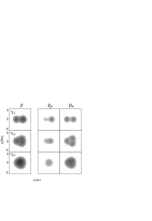
FIG. 14.: The density distributions of the normal-parity states of Li isotopes. The density of the intrinsic wave function before the parity projection is integrated along the line parallel to an appropriate principal axis as explained in the text. The AMD wave functions are obtained with the interaction (b).

In the results of Li isotopes (Fig. 14), it is easily seen that the ⁷Li system has the largest deformation with the $\alpha$+$t$ clustering structure. ⁹Li also has a deformed shape, though the deformation is not as large as the one in ⁷Li. The ground state of ¹¹Li has an almost spherical structure that can be expressed by a shell model wave function with the closed neutron $p$ shell.

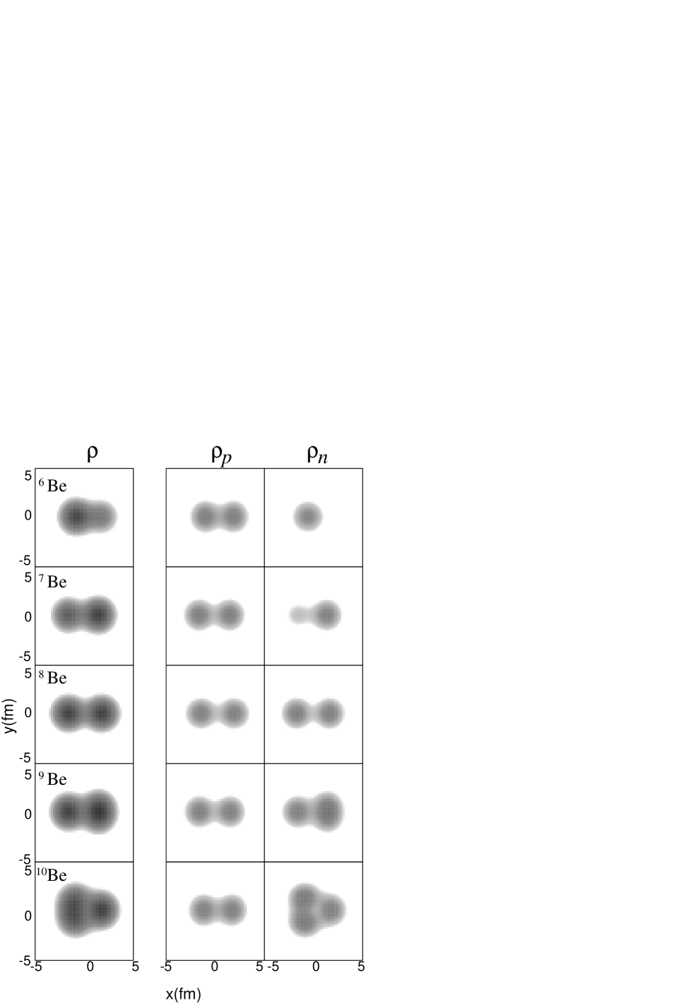
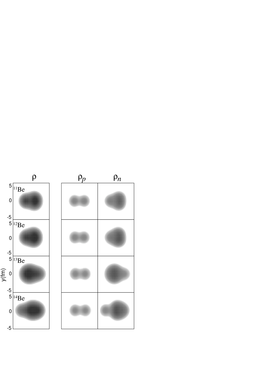
FIG. 15.: The density distributions of the normal-parity states of Be isotopes. The adopted interaction is the case (b).

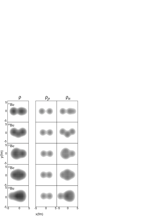
FIG. 16.: The density distributions of the non-normal-parity states of Be isotopes. The adopted interaction is the case (b).

As for the Be isotopes (Fig. 15 and 16), separated two pairs of protons are found in the proton density. It means that $2\alpha$ core exists in all the heavier Be nuclei than ⁷Be. The development of clustering in Be isotopes is estimated by the relative distance between two pairs of protons, which we show in Fig. 17. In the non-normal-parity states we find that the $2\alpha$ clustering is largest in ⁹Be as already well known. In the normal-parity states of Be isotopes, the clustering becomes weaker and weaker with the increase of neutron number up to ¹²Be with neutron magic number $N=8$. In ¹⁴Be the clustering develops again and the deformation becomes larger than ¹²Be. In the non-normal-parity states of Be isotopes, there are many exotic structures with developed clustering structures and larger deformations than the normal parity states (Fig.16). These largely deformed states give rise to the rotational bands which well agree to the experimental data of energy levels of the non-normal-parity states in ⁹Be and ¹⁰Be. The ground state of ¹¹Be is known to be a non-normal state with $1/2^{+}$. The calculated positive-parity state of ¹¹Be which corresponds to the ground $1/2^{+}$ state has the developed prolate deformation as large as the normal-parity state of ⁹Be (see Fig. 17). The deformation in the positive parity state of ¹¹Be is considered to be one of the reasons for the parity inversion of the ground state.

FIG. 17.: The distance $R_{pp}$ between two pairs of protons in the intrinsic states of the normal parity states (solid line) and the non-normal parity states (dotted line) of Be isotopes. In Be nuclei with $N\geq 4$ the distance $R_{pp}$ is considered to be the inter-cluster distance between $2\alpha$.

Here we stress again the possibility of the abnormally deformed ground state of ¹²Be. With the simple AMD calculations, the obtained normal-parity state of ¹²Be has the closed $p$-shell structure with a spherical shape of neutrons. However, the VAP calculations with the set of interaction which reproduces the abnormal spin parity $1/2^{+}$ of the ground state of ¹¹Be suggest that the ground state of ¹²Be is a $2\hbar\omega$ state with 2 neutrons in $sd$ shell in the language of a simple shell-model. In that case, the ground state of ¹²Be has a large prolate deformation with a developed clustering structure, and instead, the spherical $p$-shell closed-shell state is found in the second $0^{+}_{2}$ state. In the later section on VAP, we will mention the details about the structure of excited states of neutron-rich Be isotopes. Although the $1\hbar\omega$ and $2\hbar\omega$ states are suggested to be the ground states of Be isotopes in $N\geq 7$ region, in this section based on the simple AMD results we discuss the so-called $0\hbar\omega$ states of normal-parity states and $1\hbar\omega$ states of the non-normal parity states which are expected to be the ground or low excited states.

FIG. 18.: The density distributions of the normal-parity states of B isotopes. The intrinsic wave functions are calculated by the use of the interaction (c) with the mass-dependent Majorana parameter.

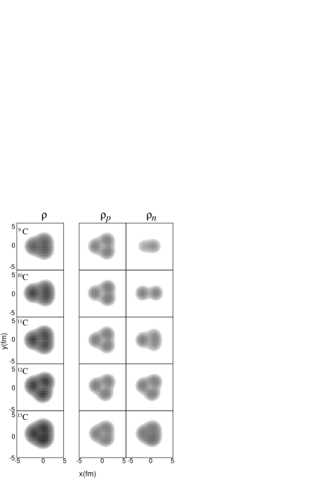
FIG. 19.: The density distributions of the normal-parity states of C isotopes. The intrinsic wave functions are calculated with the interaction (b) except for ¹⁵C. For ¹⁵C, we obtain the intrinsic state with the interaction (e).

Also in the AMD results of B isotopes shown in Fig. 18, the drastic structure change with the increase of the neutron number is found. The total matter density $\rho$ indicates the deformed state with a three-center-like clustering in ¹¹B, while the nucleus ¹³B with a neutron magic number $N=8$ has the most spherical shape among B isotopes. It is very interesting that in the neutron-richer region, ¹⁵B, ¹⁷B and ¹⁹B, the clustering structure with prolate deformation develops again. In the right column for neutron density of Fig. 18 we can see the neutron structures. In ¹¹B, six neutrons have an oblate-deformed distribution, while eight neutrons in ¹³B constitute the closed shell. On the other hands, ten neutrons in ¹⁵B posses a large prolate deformation. It is consistent with the familiar features that the ordinary nucleus ¹²C with $N=6$ has an oblate shape , the nucleus ¹⁶O with $N=8$ is spherical and ²⁰Ne with $N=10$ posses a large prolate deformation. The neutron densities in ¹⁷B and ¹⁹B are found to have largely prolately deformed structures. The prolate deformation in the system with $N=14$ is not an obvious feature, but is a characteristic seen in neutron-rich B isotopes in which five protons prefer a prolate shape. Generally speaking proton structure follows the change of neutron deformation in B isotopes. It means that in the neutron-rich region the proton density with two clusters stretches outward as the neutron number goes up toward the neutron-drip line. As a result we find that the two-center-like clustering develops more largely in ¹⁷B and most largely in ¹⁹B. It is interesting that the theory predicts the development of the clustering in B isotopes near the neutron-drip-line as well as Be isotopes. The present results for the development of clustering are consistent with the previous work by Seya et al. [47] where they calculated B isotopes by assuming the existence of a $2\alpha$ core. It should be pointed out that the present work by AMD is the first calculation which predicts the clustering structure in neutron-rich Be and B isotopes without a priori assumption of the cluster cores as far as we know. We consider that these clustering structures in the unstable nuclei near the neutron drip-line consist of cluster cores and surrounding neutron cloud because the valence neutrons are weakly bound in these nuclei. In that sense the clustering structures seen in neutron-rich region should be different from the well-known clustering structure in ordinary nuclei without valence nucleons around clusters.

In contrast to Be and B isotopes, clustering structures are not found in the normal-parity states of neutron-rich C isotopes. The results show the general tendency of the oblately deformed proton density in the C isotopes. According to the AMD calculations, the well-known $3\alpha$ clustering in ¹²C has been checked with the framework free from the assumption of the existence of clusters. The figure for neutron density (right column in Fig.19) presents the drastic change of neutron structure with the increase of the neutron number. In the neutron-rich region the neutron density stretches widely in outer region. However proton density does not change so much in spite of the drastic change of neutron structure and remains in the inner compact region. The stability of the proton structure is a characteristic of the neutron-rich C with six protons. As a result the neutron skin structure may appear in the neutron-rich C. We will make more quantitative discussions of the neutron skin in C later. In the non-normal parity states of the proton-rich C isotopes, there are many exotic shapes with the large deformation. The well-developed $3\alpha$ clustering of ¹²C seen in the negative parity states constructs a rotational $K=3^{-}$ band which well corresponds to the lowest negative-parity band observed in the experimental levels.

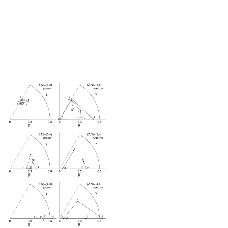
FIG. 20.: The deformation parameters of the intrinsic states of odd-even Li and B isotopes and even-even Be and C isotopes. The definitions $\beta$ and $\gamma$ are described in the text. The adopted interactions are the force (b) MV1 with $m=0.576$ for the nuclei $N\leq 8$ and the MV1 force with $m=0.63$ for the heavier nuclei $N>8$.

For the sake of the systematic study of deformations of proton density and neutron density, here we explain the deformation parameters defined by the moments $\langle x^{2}\rangle$, $\langle y^{2}\rangle$, and $\langle z^{2}\rangle$ for the intrinsic AMD wave functions as follows;

$${\langle x^{2}\rangle^{1\over 2}\over\left(\langle x^{2}\rangle\langle y^{2}\rangle\langle z^{2}\rangle\right)^{1\over 6}} \equiv {\rm exp}\left(\delta_{1}\right)={\rm exp}\left[\sqrt{5\over 4\pi}\beta{\rm cos}\left(\gamma+{2\pi\over 3}\right)\right],$$ (30)

$${\langle y^{2}\rangle^{1\over 2}\over\left(\langle x^{2}\rangle\langle y^{2}\rangle\langle z^{2}\rangle\right)^{1\over 6}} \equiv {\rm exp}\left(\delta_{2}\right)={\rm exp}\left[\sqrt{5\over 4\pi}\beta{\rm cos}\left(\gamma-{2\pi\over 3}\right)\right],$$ (31)

$${\langle z^{2}\rangle^{1\over 2}\over\left(\langle x^{2}\rangle\langle y^{2}\rangle\langle z^{2}\rangle\right)^{1\over 6}} \equiv {\rm exp}\left(\delta_{3}\right)={\rm exp}\left[\sqrt{5\over 4\pi}\beta{\rm cos}\gamma\right].$$ (32)

Here the directions $x$, $y$, and $z$ are chosen so as to satisfy the relation $\langle x^{2}\rangle\leq\langle y^{2}\rangle\leq\langle z^{2}\rangle$. The deformation parameters $\beta$ $\gamma$ calculated for protons and for neutrons are displayed in Fig. 20. The Figures are for the normal-parity states of Li, Be, B and C isotopes with the even neutron number obtained with the interaction (b) $m=0.576$ for the nuclei with $N\leq 8$ and $m=0.63$ for the nuclei with $N>8$. The behavior of the deformation parameters is not so sensitive to the Majorana parameter. It is found that the neutron shape changes rapidly with the increase of neutron number in all the series of isotopes. In the region $N\leq 12$, the main feature of deformations of the neutrons, prolate or oblate shape, is dominated only by the neutron number. It means that the neutron shape is not sensitive to the proton number in the light region. The neutron density in the system with $N=2$ has a spherical shape. In $N=4$ system the neutron density deforms prolately, and in the case of $N=6$ the neutrons prefer oblate deformation. In $N=8$ the neutron shape becomes almost spherical due to the closed neutron $p$ shell. When the neutron number becomes 10, the prolate neutron deformation appears again. As for the proton deformation, it depends on the proton number. In the system with $Z=2$, Be isotopes, the proton density prefers the prolate deformation. The degree of prolate deformation of Be isotopes changes following the drastic change of the neutron deformation. Especially the prolate deformation of protons is well developed in the system with the prolately deformed neutron density. Contrary to Be isotopes, in the case of C isotope with $Z=6$, the proton density always prefers the oblate deformation. The deformation parameter for proton is stable in spite of the change between prolate and oblate shapes of the neutron density. In the case of $Z=3$ and $Z=5$, Li and B isotopes, the proton shape depends on the neutron number so as to follow the deformed mean field given by the neutron density. In the system with the heavier neutron number such as $N=14$, the neutron shape possesses both characters, which are seen in the oblate neutron shape in ²⁰C and in the prolate deformation in ¹⁹B. In such a case with a few choice of the neutron shape, the neutron shape is determined by the proton number.

As mentioned above, in the very light region the neutron deformation is dominated by the neutron number, and the proton shape is basically determined by the proton number. The dependence of neutron(proton) shape on the neutron(proton) number is consistent with the ordinary understanding of the shell effect for the stable nuclei. That is to say the spherical shape is seen when the neutron number equals the magic number $M$, the prolate deformation at $M+2$, and oblate one at $M-2$. However one of the new features found in this study of the light unstable nuclei is that the proton shape and the neutron shape do not necessarily correlate together in light region. As a result interesting phenomena such as the opposite deformation between protons and neutrons may occur in unstable nuclei. For instance, C nuclei prefer oblate deformation of protons while neutrons tend to deform prolately when the neutron number equals to 4 and 10. Therefore ¹⁰C and ¹⁶C may have the opposite deformation between protons and neutrons. The detail of this problems in proton-rich C will be discussed later. The other interesting feature is the large deformation in the nuclei with prolate protons and prolate neutrons. The developments of deformations in ⁸Be, ¹⁴Be, ¹⁵B, ¹⁷B, and ¹⁹Be are understood as follows. Once a prolate shape of protons is chosen by the proton number, the prolate deformation is enhanced and the clustering of protons is developed by the neutron deformations if the neutrons deform prolately.

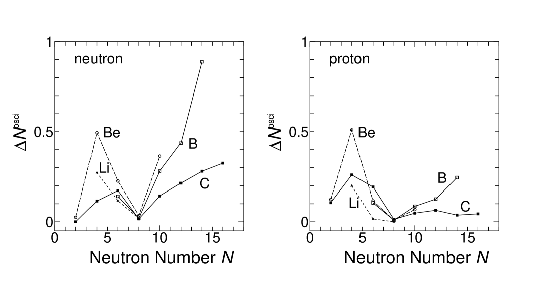
FIG. 21.: The deviation of the proton orbits and neutron orbits from the harmonic oscillator shell-model wave functions in the normal-parity states obtained with AMD calculations. The expectation values of the total number of the oscillator quanta are calculated with the spin-parity eigen states projected from the intrinsic AMD wave functions. The detail is mentioned in the text. The interaction (b) MV1 with $m=0.576$ is used in the region $N\leq 8$, and the MV1 force with $m=0.63$ is adopted in the region $N>8$.

In order to analyze clustering development quantitatively, we calculate the expectation values for the total number of the oscillator quanta. In general if the clustering structure develops the wave function of the system contains the components of a large amount of the orbits in higher shells, therefore the the expectation values of the oscillator quanta become larger. On the other hands a small value of the oscillator quantum indicates that the state is almost written by the shell-model states in the $0\hbar\omega$ configurations but the spatial clustering does not exist. We introduce the value $\Delta N_{p}$ ($\Delta N_{n}$) which stands for the deviation of the proton (neutron) orbits in the AMD wave function from those in the $0\hbar\omega$ states of the harmonic oscillator shell model basis,

$$\Delta N_{p}\equiv\frac{\langle P^{J\pm}_{MK}\Phi_{AMD}|{N}^{op}_{p}|P^{J\pm}_{MK}\Phi_{AMD}\rangle}{\langle P^{J\pm}_{MK}\Phi_{AMD}|P^{J\pm}_{MK}\Phi_{AMD}\rangle}-N^{min}_{p},$$ (33)

$$\Delta N_{n}\equiv\frac{\langle P^{J\pm}_{MK}\Phi_{AMD}|{N}^{op}_{n}|P^{J\pm}_{MK}\Phi_{AMD}\rangle}{\langle P^{J\pm}_{MK}\Phi_{AMD}|P^{J\pm}_{MK}\Phi_{AMD}\rangle}-N^{min}_{n},$$ (34)

where $N^{op}_{p}$ and $N^{op}_{n}$ are the oscillator quantum number operators and $N^{min}_{p}$ ($N^{min}_{n}$) are the minimum values of oscillator quantum numbers for protons (neutrons) given by the $0\hbar\omega$ state. We choose the same width parameters for $N^{op}_{p}$ and $N^{op}_{n}$ as the width of the Gaussians in the AMD wave functions for simplicity. In Fig. 21, $\Delta N_{p}$ and $\Delta N_{n}$ for the normal parity states are displayed as a function of neutron number. We can estimate the clustering development by the deviation of proton orbits $\Delta N_{p}$ from the $0\hbar\omega$ state. As is expected, the dependence of $\Delta N_{p}$ of Be isotopes on the neutron number is found to be very similar to the that of the inter-cluster distance between $2\alpha$ which has been already shown in Fig.17. In the Li, Be, and B isotopes the neutron number dependence of $\Delta N_{p}$ is qualitatively similar to the behavior of $\Delta N_{n}$ for neutrons. It is because the development of the clustering structure in these isotopes is sensitive to the neutron structure determined by the neutron number. In the Be and B isotopes, the increase of $\Delta N_{p}$ in the region $N>8$ indicates that the clustering develops as the neutron number increases toward the neutron-drip line. In all the nuclei with $N=8$, the $\Delta N_{n}$ and also $\Delta N_{p}$ are almost zero, which stands for that the states are approximately same with the shell-model states and can be written by the major shell orbits. We stress again that we analyzed the structure change of the normal-parity states where the main components are $0\hbar\omega$ states even if they are not necessarily ground states. The effect of the neutron magic number $N=8$ is clearly seen in the valley at $N=8$ in the variation of $\Delta N_{p}$. In the case of the C isotopes, the large $\Delta N_{p}$ at $N=6$ indicates the developed clustering structure in ¹²C, while the small values of $\Delta N_{p}$ in the region $N\geq 8$ are because of the disappearance of clustering in the neutron-rich C as already mentioned.

2 Effects of intrinsic structures on electromagnetic properties

Here we consider the effect of clustering structures on the observable electric and magnetic moments by analyzing $\mu$ and $Q$ moments of the ground states in Li and B isotopes. As shown above the simple AMD calculations well agree to the experimental data of the electromagnetic properties such as the magnetic dipole moments $\mu$ and the electric quadrupole moments $Q$, the strength of transitions. Roughly speaking, the electromagnetic properties of the odd-even nucleus reflect the orbit of the last valence proton. In that sense the last proton in $p$-shell may dominate the moments in the odd-even Li and B isotopes, however, $\mu$ and $Q$ moments in these nuclei shift as functions of the neutron number (Fig. 11 and 12). The $N$ dependence of the experimental data of the electric and the magnetic properties can be explained in relation to the drastic change between the cluster and shell-model-like structures.

In the following discussion, we consider two kinds of the fundamental effects of the cluster structures on the properties such as the electric and magnetic moments. One is caused by the spatial relative distance between clusters (spatial clustering effects), and the other is concerned with the angular momentum coupling correlation of nucleons. As a typical example of the latter effect, we recall the so-called shell-model cluster in the SU³ coupling shell-model [48, 49] configuration. As we show below, it is found that the effect of the cluster structure on the magnetic dipole moments of Li and B isotopes is given only by the cluster coupling of angular momenta, while the quadrupole moments are effected by the spatial cluster as well as the cluster coupling of angular momenta. In order to extract the effect of the cluster coupling of angular momenta from the AMD wave functions, we have artificially made the inter-cluster relative distances in the AMD wave functions very small so as to obtain the states in the shell-model limit. In the obtained shell-model limit states, the spatial cluster is not recognizable any more but only the effects of the cluster coupling of angular momenta persist.

TABLE VII.: The expectation values of the magnetic dipole operator $\mu$, the electric quadrupole operator $Q$, the square of total orbital-angular-momenta of protons $\langle{\bf L}^{2}_{p}\rangle$, the square of total orbital-angular-momenta of neutrons $\langle{\bf L}^{2}_{n}\rangle$, the square of total orbital-angular-momenta of the system $\langle{\bf L}^{2}\rangle$, the total intrinsic spin of protons $\langle{\bf S}^{2}_{p}\rangle$, the total intrinsic spin of neutrons $\langle{\bf S}^{2}_{n}\rangle$, and the total intrinsic spin of the system $\langle{\bf S}^{2}\rangle$ for the highest states $|{3\over 2}{3\over 2}\rangle$ in the simplest AMD calculations of Li and B isotopes. Those in the shell-model limit are also listed.

		$\mu$	$Q$	$\langle{\bf L}^{2}_{n}\rangle$	$\langle{\bf L}^{2}_{p}\rangle$	$\langle{\bf L}^{2}\rangle$	$\langle{\bf S}^{2}_{n}\rangle$	$\langle{\bf S}^{2}_{p}\rangle$	$\langle{\bf S}^{2}\rangle$
		($\mu_{N}$)	(e$\cdot$mb)
	EXP.	3.27	$-$40(3)
7 Li	AMD	3.15	$-$27.6	2.8	2.2	2.0	0.00	0.75	0.75
	SML	3.14	$-$15.1	2.6	2.0	2.0	0.00	0.75	0.75
	EXP.	3.44	$-$27(1)
9 Li	AMD	3.42	$-$27.0	1.1	2.0	2.1	0.13	0.75	0.90
	SML	3.44	$-$23.2	1.1	2.0	2.0	0.13	0.75	0.90
	EXP.	3.76	$-$31(5)
11 Li	AMD	3.79	$-$29.4	0.0	2.0	2.0	0.00	0.75	0.75
	SML	3.79	$-$29.4	0.0	2.0	2.0	0.00	0.75	0.75
	EXP.	2.69	40
11 B	AMD	2.65	34.0	2.5	3.6	2.8	0.04	0.75	0.78
	SML	2.66	25.9	2.3	3.4	2.8	0.04	0.75	0.78
	EXP.	3.17	37(4)
13 B	AMD	3.17	31.7	0.0	2.7	2.7	0.00	0.75	0.75
	SML	3.18	28.6	0.0	2.7	2.7	0.00	0.75	0.75
	EXP.	2.66	38(1)
15 B	AMD	2.63	34.3	3.7	3.8	2.8	0.00	0.75	0.75
	SML	2.64	22.5	3.5	3.7	2.8	0.00	0.75	0.75
	EXP.	$2.54$	$-$
17 B	AMD	2.49	42.2	4.4	4.1	2.9	0.07	0.75	0.81
	SML	2.50	22.6	4.0	3.7	2.9	0.33	0.75	0.77
	EXP.	$-$	$-$
19 B	AMD	2.53	50.8	4.3	4.2	2.90	0.00	0.75	0.75
	SML	2.55	24.9	3.9	3.8	2.9	0.00	0.75	0.75

TABLE VIII.: The expectation values of the $z$-components of the operators which effect on the $\mu$ moments; the total orbital-angular-momenta of protons $\langle L_{pz}\rangle$, the total orbital-angular-momenta of neutrons $\langle L_{nz}\rangle$, the total intrinsic spin of protons $\langle S_{pz}\rangle$, and the total intrinsic spin of neutrons $\langle S_{nz}\rangle$, for the highest states $|{3\over 2}{3\over 2}\rangle$ in the simplest AMD calculations and in the shell-model limit for Li and B isotopes.

		$\langle S_{pz}\rangle$	$\langle S_{nz}\rangle$	$\langle L_{pz}\rangle$	$\langle L_{nz}\rangle$
7 Li	AMD	0.50	0.00	0.36	0.64
	SML	0.50	0.00	0.35	0.65
9 Li	AMD	0.50	0.02	0.71	0.27
	SML	0.50	0.02	0.72	0.26
11 Li	AMD	0.50	0.00	1.00	0.00
	SML	0.50	0.00	1.00	0.00
11 B	AMD	0.34	0.00	0.74	0.41
	SML	0.34	0.00	0.74	0.41
13 B	AMD	0.37	0.00	1.13	0.00
	SML	0.37	0.00	1.13	0.00
15 B	AMD	0.33	0.00	0.77	0.40
	SML	0.34	0.00	0.77	0.40
17 B	AMD	0.33	0.00	0.68	0.49
	SML	0.33	0.00	0.68	0.49
19 B	AMD	0.33	0.00	0.73	0.45
	SML	0.33	0.00	0.73	0.45

Table VII shows the results of $\mu$ and $Q$ moments calculated with the spin-parity projected states from the shell-model limit wave functions, which are compared with the original AMD results. In the table we also list the expectation values of the squared total-angular momenta ${\bf J}_{p}$, ${\bf J}_{n}$, ${\bf J}$, the orbital-angular momenta ${\bf L}_{p}$, ${\bf L}_{n}$, ${\bf L}$ and the intrinsic spins ${\bf S}_{p}$, ${\bf S}_{n}$, ${\bf S}$ for protons, neutrons and for the total system, which have close relations with the spin configurations. We also calculate the $z$-components of the orbital-angular momenta and the intrinsic spins of protons and neutrons in the highest $M$ states $|JM\rangle=|\frac{3}{2}\frac{3}{2}\rangle$. Since the $\mu$ moments in the shell-model limit are found to be almost the same as those of the original AMD, it is confirmed that the magnetic dipole moments do not depend on the spatial clustering but are effected only by the cluster coupling of angular momenta. It is easily understood because the expectation values of linear terms of operators, J, L and S are mainly determined by the cluster coupling of angular momenta. As shown in the Table VII the magnitude of the total neutron intrinsic spin almost equals to 0 because the intrinsic spins of the even neutrons are almost paired off. It means that the direct contribution to the $\mu$ moments from the neutrons is little. Then the $\mu$ moments of odd-even Li and B isotopes approximately consist of two terms from $z$-components of ${\bf S}_{p}$ and ${\bf L}_{p}$,

$$\mu\approx\mu_{s}+\mu_{l}$$ (36)

$$\mu_{s}\equiv 5.58\langle{3\over 2}{3\over 2}|S_{pz}|{3\over 2}{3\over 2}\rangle\mu_{N},\mu_{l}\equiv\langle{3\over 2}{3\over 2}|L_{pz}|{3\over 2}{3\over 2}\rangle\mu_{N},$$ (37)

where $\mu_{N}$ stands for the nuclear magneton. Figure 22 presents the components from the two terms $\mu_{s}$ and $\mu_{l}$ in the total $\mu$ moments.

FIG. 22.: The effects due to the intrinsic spins $\mu_{s}$ and of the orbital-angular momentum $\mu_{l}$ on the total magnetic dipole moments $\mu$ of Li and B isotopes. The experimental data are also shown with square points.

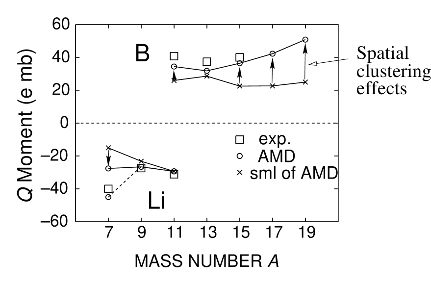
FIG. 23.: The $Q$ moments of Li and B isotopes for the original AMD wave functions and the shell-model limit described in the text. Squares are the experimental data. The spatial clustering effects can be estimated by subtracting the $Q$ moments (cross points ) in the shell-model limit from the original results (open circles).

In the Li isotopes, $\mu_{s}$ is almost constant because $|{\bf S}_{p}|={1\over 2}$ and $S_{pz}=0.5$ (see Table VIII). The deviation of $\mu$ from the Schmidt value and its $N$ dependence originate from the latter terms $\mu_{l}$ due to the orbital-angular momentum of protons. The reason of the $N$ dependence of $\mu_{l}$ can be understood as follows. The total angular momenta $|{\bf L}|$ are always 1 and $L_{z}=1.0$ in Li isotopes. However the state with the cluster coupling contains the components of $|{\bf L}_{n}|\neq 0$ states with non-zero total-orbital-angular momentum of neutrons, which makes $L_{pz}$ decrease in the highest $|{3\over 2}{3\over 2}\rangle$ states. That is why ⁷Li with the clustering structure has the smallest $\mu$ moments in odd-even Li isotopes. In other words, the $N$ dependence of $\mu$ moments of Li isotopes is described by the non-zero ${\bf L}_{n}$ of neutrons due to the clustering coupling effects.

In the case of B isotopes, the deviations of the $\mu$ moments from the Schmidt value 3.79$\mu_{N}$ for the $p_{3/2}$ proton orbit are not as small as the case of Li isotopes. In B isotopes the $z$-component $\langle S_{pz}\rangle$ has proved to be about 0.35 which gives a smaller magnitude $\mu_{s}\approx 1.8\mu_{N}$ than the case of $\langle S_{pz}\rangle=0.5$. In the results in Table VII, it is found that the calculated values of $\langle{\bf L}^{2}\rangle$ are almost constantly 2.8 in B isotopes and 2.0 in Li isotopes. It implies that the wave functions of Li isotopes are the almost pure $L=1$ states, while those of B isotopes contains $L=1$ states and $L=2$ whose components are easily estimated to be about 20%. The mixing of the $L=2$ states in B isotopes makes ${\bf S}_{p}$ tilted from the $z$ direction in the $|JM\rangle=|{3\over 2}{3\over 2}\rangle$ states as to $S_{pz}\approx 0.35$. The reason of the pure $L=1$ state in Li and the mixing ratio of the $L=2$ states in B are described in Ref.[30] in more detail. The second term $\mu_{l}$ causes the $N$ dependence of $\mu$ moments of B isotopes as similar way with Li isotopes. Even though the magnitude $|{\bf L}|$ and the $z$-component $\langle L_{z}\rangle$ of the total-orbital-angular momentum is approximately constant in the B isotopes, the clustering gives the components of ${\bf L}_{n}\neq 0$ states which reduce the magnitude of $\langle L_{pz}\rangle$. Because of such a effect of the clustering coupling on the $\mu_{l}$ term, the magnetic moments of ¹¹B, ¹⁵B, ¹⁷B and ¹⁹B are smaller than the one of ¹³B which has the shell-model like structure. Since the closed neutron shell in the nuclei ¹³B with $N=8$ make ${\bf S}_{n}={\bf L}_{n}={\bf J}_{n}=0$, the $\mu$ moments of ¹³B is the largest in B isotopes. Similarly to Li isotopes, it is concluded that the $N$ dependence of $\mu$ moments of B isotopes is understood by the cluster coupling effect.

In contrast to the magnetic dipole moments, the electric quadrupole moments are sensitive to the relative distance between clusters. For the sake of estimating the spatial cluster effects on $Q$ moments, we try to decompose the calculated $Q$ moments into two components: The first component is originated by the spatial clustering, and the other is due to other properties including the cluster coupling of angular momenta. We consider that the second components are given by the $Q$ moments calculated by the shell-model-limit wave function where the spatial clustering has been already removed. They are shown in Table VII together with the $Q$-moments of the AMD calculations. We display the two components in $Q$ moments in the Fig. 23, which is helpful to analyze the $N$ dependence of the each component. As for the B isotopes the calculated $Q$ moments in the shell model limit are 25.9, 28.6, 22.5, 22.6 and 24.9 e$\cdot$mb for ¹¹B, ¹³B, ¹⁵B, ¹⁷B and ¹⁹B, respectively. It shows that the second components in these nuclei except for ¹³B are smaller than the one in ¹³B with $N=8$. With similar argument as for $\mu$-moments, we expect that the reduction of the $Q$-moments in other B isotopes than ¹³B should be explained by the mixing of the component of the non-zero neutron orbital-angular momentum. By subtracting these second components from the total $Q$-moments ( namely the $Q$-moments of the AMD calculations ), we can estimate the contribution of the first component due to the spatial clustering as 8.1, 3.1, 11.8, 19.6 and 25.9 e$\cdot$mb for ¹¹B, ¹³B, ¹⁵B, ¹⁷B and ¹⁹B, respectively. This component is smallest in ¹³B and becomes larger as the neutron number increases toward the neutron drip-line. Such dependence on $N$ of the first component is indeed consistent with the clustering development mentioned in the previous subsection. In the case of Li isotopes the first component is largest in ⁷Li and decreases toward ¹¹Li as the clustering structure weakens.

Thus it is proved that the systematic $N$-dependent features of experimental data for the electric magnetic properties are quantitatively explained by the structure change given by our AMD results. The reader is referred to Ref.[30] for the detailed discussions.

3 Opposite deformation between protons and neutrons

As mentioned above, AMD results suggest that the opposite deformations between protons and neutrons may be found in the proton-rich C isotopes. In Fig. 24, we illustrate the deformation parameters of protons and neutrons in proton-rich C isotopes. It is notable that the neutrons prefer the prolate and the triaxial deformations rather than the oblate shape in these nuclei because of the neutron number $N=3,4,5$. On the other hands, the protons prefer oblate shape in C isotopes. As a result the disagreement between the proton and the neutron deformations is found in proton-rich C. Our purpose here is to confirm the disagreement between the proton and the neutron shapes by the help of the electric quadrupole moments and transitions in C and the ones in the mirror nuclei.

First we discuss $Q$ moments of ¹¹C and the mirror nucleus ¹¹B. Based on mirror symmetry for proton and neutron deformations, we compare the proton and the neutron deformations by analyzing the ratio of the electric quadrupole moment $Q$ in ¹¹C to the one in ¹¹B. We introduce the well-known approximate relation between the electric quadrupole moment $Q$ in the laboratory frame and the intrinsic quadrupole moment $Q_{0}$;

$$Q=Q_{0}{3K^{2}-J(J+1)\over(2J+3)(J+1)}.$$ (38)

By using Eq. 32 we can express the intrinsic electric quadrupole moment $Q_{0}$ as follows in the first order of the deformation parameter $\beta_{p}$,

$$Q_{0}=\sqrt{16\pi\over 5}{3\over 4\pi}Ze\beta_{p}{\rm cos}\gamma_{p}R_{e}^{2},$$ (39)

where $\beta_{p}$ and $\gamma_{p}$ are the deformation parameters for the proton density, and $Z$ and $R_{e}$ are the proton number and the charge radius, respectively. Instead of the usual deformation parameter $\beta_{p}$ in the usual equation $Q_{0}=\sqrt{16\pi\over 5}{3\over 4\pi}Ze\beta_{p}R_{e}^{2}$, we introduce the effective deformation parameter $\beta_{p}{\rm cos}\gamma_{p}$ in Eq.39 which is necessary for the system with different proton and neutron shapes as described below. We explain the appropriate principal axes in the nucleus where the different proton and neutron shapes coexist as shown in schematic Figure 25. For example in the nucleus with oblate proton and prolate neutron deformations, the approximate symmetry axis $x$ for protons usually differs from the approximate symmetry axis $z$ for neutrons so as to make the largest overlap between the proton density and the neutron density. In many cases, it has been found that a symmetry axis $z$ for the prolate neutron density should be chosen as the principal axis $Z$ of the total intrinsic system for the total-angular momentum projection in generating the lowest $J^{\pm}$ state with an approximately good $K$ quantum. In such cases, the usual formula for $Q_{0}$ should be modified by using the effective deformation to $z$-axis, $\beta_{p}$cos$\gamma_{p}$ instead of $\beta_{p}$. In other words, an oblate deformation gives a smaller contribution to the intrinsic quadrupole moment $Q_{0}$ than is expected.

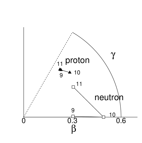
FIG. 24.: Deformation parameters $(\beta,\gamma)$ for proton and neutron densities in the intrinsic states of proton-rich C isotopes with $A=9\sim 11$ are given by triangles and squares, respectively. The mass number $A$ is indicated beside each point in the figure. The interaction (b) is used.

FIG. 25.: Schematic figures of the nucleus with oblate proton and prolate neutron deformations. In the body-fixed flame $x,y,z$ is chosen so that moments of inertia obey the relation ${\cal I}_{zz}\leq{\cal I}_{yy}\leq{\cal I}_{xx}$.

Assuming these simple approximations the ratio of the $Q$ moment in ¹¹C to that in ¹¹B is represented by the product of three terms, the ratio of proton numbers, that of the proton deformation parameters, and the one of the charge radii. When we assume the mirror symmetry for the deformation parameters and replace the deformation parameter $\beta_{p}{\rm cos}\gamma_{p}(^{11}$B) of the proton density in ¹¹B by $\beta_{n}{\rm cos}\gamma_{n}(^{11}$C) of the neutron density in ¹¹C, the ratio of $Q$ is written as,

$${Q(^{11}{\rm C})\over Q(^{11}{\rm B})}=\left({Z=6\over Z=5}\right)\times\left({\beta_{p}{\rm cos}\gamma_{p}\left({}^{11}{\rm C}\right)\over\beta_{n}{\rm cos}\gamma_{n}\left({}^{11}{\rm C}\right)}\right)\times\left({R_{e}(^{11}{\rm C})\over R_{e}(^{11}{\rm B})}\right)^{2}.$$ (40)

We take the third term for the charge radii to be unity since ¹¹C and ¹¹B are the nuclei close to the stability line. If the neutron deformation agrees to the proton deformation in ¹¹C, the second term gives no contribution to the ratio of $Q$ moments and the ratio can be explained only by the charge ratio 1.2. However the ratio $0.88$ deduced from the experimental data is less than a unity and is inconsistent with the $Z$ ratio because the experimental data of $Q(^{11}$C)=34.8 e$\cdot$mb is smaller than $Q(^{11}$B)=40.7 e$\cdot$mb. According to AMD calculations, this problem can be resolved by taking into account the difference between the intrinsic deformations of proton and neutron densities in ¹¹C. Through the second term in Eq.(40), the ratio of $Q$ moments reflects the difference of intrinsic shapes between proton and neutron densities. As shown above in Fig.24 the proton deformation is oblate while the neutron density becomes a triaxial shape in ¹¹C. Since $\beta_{p}{\rm cos}\gamma_{p}(^{11}$C) is smaller than $\beta_{n}{\rm cos}\gamma_{n}(^{11}$C), the second term in Eq. 40 becomes less than unity, which cancels the effect of the first term of the $Z$ ratio.

We make further quantitative discussion by the use of theoretical values of deformation parameters in the intrinsic states obtained with AMD. In the present results, the ground state of ¹¹C with $J=3/2$ is obtained by a total-angular-momentum projection on a state $|J=3/2,K=3/2\rangle$ with respects to the principal $z$ axis with the minimum moment of inertia. Using the theoretical values of $\beta_{p}{\rm cos}\gamma_{p}$ and $\beta_{n}{\rm cos}\gamma_{n}$ shown in Fig.24 we can estimate the ratio of $Q$ moments with the first and the second terms in Eq.40. The estimated ratio is found to be 0.87 which is as small as the value of 0.88 deduced from the experimental data. In fact the theoretical results of electric $Q$ moments for total-angular momentum projected states are 20 e$\cdot$mb for ¹¹C and 34 e$\cdot$mb for ¹¹B, which are consistent with the experimental data of $Q(^{11}$C)$<Q(^{11}$B) (Table.IX).

TABLE IX.: Electric quadrupole moments and transitions of proton-rich C isotopes and the mirror nuclei. Calculations are with MV1 force ($m=0.576$) and the experimental data are taken from Ref.[46].

		electric $Q$ moments
nucleus	level	exp.	theory
11C	$3/2^{-}$	34.3 e$\cdot$mb	20 e$\cdot$mb
11B	$3/2^{-}$	40.7(3) e$\cdot$mb	34 e$\cdot$mb
10C	$2^{+}$	$-$	$-38$ e$\cdot$mb
10Be	$2^{+}$	$-$	$-65$ e$\cdot$mb
9C	$3/2^{-}$	$-$	$-28$ e$\cdot$mb
9Li	$3/2^{-}$	$-27.8$ e$\cdot$mb	$-27$ e$\cdot$mb
		$E2$ transition strength
nucleus	level	exp.	theory
11C	$5/2^{-}\rightarrow 3/2^{-}$	$-$	6.8 e${}^{2}{\rm fm}^{4}$
11B	$5/2^{-}\rightarrow 3/2^{-}$	13.9(3.4) e${}^{2}{\rm fm}^{4}$	11.3 e${}^{2}{\rm fm}^{4}$
10C	$2^{+}\rightarrow 0^{+}$	12.3(2.0) e${}^{2}{\rm fm}^{4}$	5.3 e${}^{2}{\rm fm}^{4}$
10Be	$2^{+}\rightarrow 0^{+}$	10.5(1.0) e${}^{2}{\rm fm}^{4}$	9.5 e${}^{2}{\rm fm}^{4}$
9C	$1/2^{-}\rightarrow 3/2^{-}$	$-$	5.7 e${}^{2}{\rm fm}^{4}$
9Li	$1/2^{-}\rightarrow 3/2-$	$-$	7.2 e${}^{2}{\rm fm}^{4}$

It is concluded that the difference of the intrinsic deformation of the proton density in ¹¹C from that in ¹¹B (an oblate shape in ¹¹C and a triaxial shape in ¹¹B) makes significant effects to the ratio of the $Q$ moment of ¹¹C to that of ¹¹B. By assuming the mirror symmetry, it is theoretically suggested that the disagreement between proton and neutron deformations in ¹¹C is supported by the experimental fact of the ratio $Q(^{11}$C)/$Q(^{11}$B)/ less than a unity.

Next we make similar analysis of the deformations for ¹⁰C. We find that the difference between proton and neutron deformations in ¹⁰C is important to understand the ratio of the $E2$ transition strength $B(E2;2^{+}\rightarrow 0^{+})$ in ¹⁰C to that in the mirror nucleus ¹⁰Be. Assuming mirror symmetry, the ratio of $B(E2)$ is approximated similarly to Eq.40 as,

$${B(E2;^{10}{\rm C})\over B(E2;^{10}{\rm Be})}=\left({Z=6\over Z=4}\right)^{2}\times\left({\beta_{p}{\rm cos}\gamma_{p}\left({}^{10}{\rm C}\right)\over\beta_{n}{\rm cos}\gamma_{n}\left({}^{10}{\rm C}\right)}\right)^{2}\times\left({R_{e}(^{10}{\rm C})\over R_{e}(^{10}{\rm Be})}\right)^{4}.$$ (41)

The first term of the charge ratio $(6/4)^{2}$=2.25 is much larger than the ratio of experimental values 12.3(2.0)e²fm⁴/10.5(1.0)e²fm⁴ =1.2(0.3). The reason why the square of the charge ratio fails to reproduce the ratio of $B(E2)$ in the mirror nuclei ¹⁰C and ¹⁰Be is because of the disagreement between proton and neutron deformations in ¹⁰C.

In the intrinsic state of ¹⁰C, the proton density deforms oblately with $\beta_{p}{\rm cos}\gamma_{p}=0.28$ while the neutron deformation is prolate with a larger value of the effective deformation parameter $\beta_{n}{\rm cos}\gamma_{n}$=0.49 (Fig.24), which makes the second term in Eq.41 less than unity. If the third term is omitted, the ratio is roughly estimated as,

$${B(E2;^{10}{\rm C})\over B(E2;^{10}{\rm Be})}=2.25\times(0.28/0.49)^{2}\sim 0.75.$$ (42)

Although the ratio estimated above is smaller than the ratio 1.2 deduced from the experimental data, it is found that the reduction of the ratio of the proton numbers is made by the ratio of the deformation parameters The microscopic calculations of $Q$ moments with AMD are shown in Table IX and are compared with the experimental data. Since the calculations underestimate the value of $B(E2;^{10}$C), the ratio $B(E2;^{10}$C)$/B(E2;^{10}$Be) is smaller than a unity. In the results with VAP calculation which will be mentioned later, the theoretical value of $B(E2;^{10}$C) is improved.

As for the ⁹C and the mirror nucleus ⁹Li, the present prediction is that the $Q$ moments of ⁹C is smaller to the one of ⁹Li. We should note that the present results do not include the effect of the long tail of valence nucleons. However, if the proton halo of ⁹C exists because the separation energy of protons is small, the orbits of the valence protons may give the large effect on the $Q$ moments.

4 Neutron skin and halo

The presence of a neutron skin structure has been discussed for a long time. Recently thick neutron skins have been reported in He isotopes [50] and in ²⁰N [51] by the help of the experimental data of interaction cross sections. The appearance of the neutron skin has been also shown in the comparison of neutron radii with proton radii along a chain of Na isotopes by combining the data of the isotope-shift for charge radii with those of the matter radii deduced from interaction cross sections [52]. Also the theoretical studies of skin structures have been tried in unstable nuclei [22, 30, 44, 53].

The present results suggest that in the neutron-rich nuclei of B and C isotopes the density of neutrons stretches far toward the outer region. The simple AMD calculations predict the presence of “neutron skin structure”, which is the surface region with rather high neutron density but low proton density. In particular, C isotopes are expected to have thicker skins than those of B isotopes because the neutron-rich C have no developed clustering structure as is seen in the proton density of ²⁰C which remains in the inner region as compact as that of stable C nuclei. One of characteristics of C isotopes is the stationary structure of protons in spite of the drastic change of neutron structure along the increase of neutron number. It is in contrast with neutron-rich B isotopes which are predicted to have the clustering structure. According to simple AMD calculations, in a series of $N=14$ isotones the neutron skin which is developed in ²⁰C weakens with the increase of the proton number because the mean-field for the neutrons given by proton density becomes deeper to decrease the neutron radii.

FIG. 26.: The densities $\rho_{p}$ of protons and $\rho_{n}$ of neutrons as a function of radius in C isotopes. The densities of the $0^{+}$ states are obtained with AMD calculations by using MV1 force with $m=0.63$. The proton density of ¹²C is written by the dotted lines. The densities of in ¹⁹B are also shown together with the proton density of ¹³B.

Figure 26 shows the proton and the neutron densities of C isotopes as a function of radius. The difference between proton and neutron densities in the surface region around $r\approx 4$ fm enhances as the neutron number increases from $N=10$ toward the neutron-drip line. In the surface region of ²⁰C, the line for the neutron density (solid) seems to be shifted outward by about 1 fm compared with the line for proton density (dashed).

FIG. 27.: Theoretical values of root-mean-square radii of protons (dotted lines) and neutrons (solid lines). Calculations are the results with the interaction (b) MV1 ($m=0.576$) and with the MV1 force with $m=0.63$.

As already mentioned the recently measured radii of C isotopes [43] agree well systematically with the simple AMD calculations except for ¹⁹C which is expected to have a neutron halo structure (Fig. 10). We show the root-mean-square radii of neutrons and protons separately in Fig.27. It is found that the neutron radii become larger and larger in the region heavier than ¹⁴C while the proton radii are rather stable with the increase of the neutron number. Although the radii depend on the adopted interaction parameters, in both calculations with Majorana parameter $m=0.576$ and $m=0.63$ the difference between the proton radius and the neutron radius in ²⁰C is more than 0.3 fm. According to the present results, the increase of the matter radii in the neutron-rich C isotopes is mainly due to the development of the neutron skin structure.

The radial behavior of the densities of protons and neutrons is related closely with the single-particle energies. We calculate the single-particle energies and the single-particle wave functions by diagonalizing the single-particle Hamiltonian with the analogy to Hartree-Fock theory. First we transform the set of single-particle wave functions $\varphi_{i}$ of the solved of AMD wave function into an orthonormal base $\tilde{\varphi}_{\alpha}$. The single-particle Hamiltonian can be constructed by the use of the orthonormal base as follows [44, 37, 39];

$$h_{\alpha\beta} = \langle\tilde{\varphi}_{\alpha}|\hat{t}|\tilde{\varphi}_{\beta}\rangle+\sum^{A}_{\gamma}\langle\tilde{\varphi}_{\alpha}\tilde{\varphi}_{\gamma}|\hat{v}|\tilde{\varphi}_{\beta}\tilde{\varphi}_{\gamma}-\tilde{\varphi}_{\gamma}\tilde{\varphi}_{\beta}\rangle$$ (43)

$$+ {1\over 2}\sum^{A}_{\gamma,\delta}\langle\tilde{\varphi}_{\alpha}\tilde{\varphi}_{\gamma}\tilde{\varphi}_{\delta}|\hat{v}_{3}|\tilde{\varphi}_{\beta}\tilde{\varphi}_{\gamma}\tilde{\varphi}_{\delta}+\tilde{\varphi}_{\delta}\tilde{\varphi}_{\beta}\tilde{\varphi}_{\gamma}+\tilde{\varphi}_{\gamma}\tilde{\varphi}_{\delta}\tilde{\varphi}_{\beta}-\tilde{\varphi}_{\beta}\tilde{\varphi}_{\delta}\tilde{\varphi}_{\gamma}-\tilde{\varphi}_{\gamma}\tilde{\varphi}_{\beta}\tilde{\varphi}_{\delta}-\tilde{\varphi}_{\delta}\tilde{\varphi}_{\gamma}\tilde{\varphi}_{\beta}\rangle,$$ (44)

where the Hamiltonian operator is written by a sum of the kinetic term, the two-body interaction term and the three-body interaction term; $H=\sum_{i}\hat{t}+\sum_{i<j}\hat{v}_{2}+\sum_{i<j<k}\hat{v}_{3}$. We note that the single-particle energies defined as above can be positive because the model space for single particle wave functions is restricted to the Gaussian wave packet giving rise to an artificial wall due to the zero-point kinetic energy of the packet which prevents the single-particle wave function from escaping out of the nucleus. In Fig.28 we present single-particle energies in C isotopes which are calculated from the obtained intrinsic AMD wave functions. It is found that in the neutron-rich C isotopes heavier than ¹⁴C the Fermi energy is at most a few MeV. In the nuclei near the neutron-drip line, many valence neutrons occupy the higher orbits a few MeV below the zero energy which correspond to $sd$ orbits. These weakly bound neutrons build the neutron skin structure. In the even-odd neutron-rich C isotopes such as ¹⁹C, the energy of the last valence neutron is about zero energy. The possible existence of halo structure in ¹⁹C is suggested experimentally by the measurements of the longitudinal-momentum distribution of ¹⁸C after the one-neutron breakup of ¹⁹C [13] and also by the interaction cross sections [43]. Although the halo structure may not be seen in the present results because the AMD wavefunction is not sufficient to describe a long tail of the halo tail, considering the small binding energy of valence neutrons we naturally expect that the halo structure may appear if the single-particle wave function of such a loosely bound valence neutron is described more precisely than the present model space.

FIG. 28.: The single-particle energies of the intrinsic states for the normal parity states of C isotopes. The method to calculate the single-particle energies is explained in the text. The energies of proton(neutron) orbits are presented on the left(right). The MV1 force with $m=0.63$ is used.

On the other hands, the protons are deeply bound in the neutron-rich C. The binding energies of protons grow rapidly from ⁹C to ¹⁴C because the number of neutrons in $p$ shell increases. In the heavier region from ¹⁴C to the neutron-drip line, the proton energy becomes deeper and deeper gradually. Taking into account the potential depth of protons and the enlargement of the neutron density distribution, the kink of radii at ¹⁴C seems to be a natural phenomenon which reflects the shell effect of neutrons at $N=8$.

V Study with VAP

Recently the structures of the excited states as well as the ground states are very attractive in the study of unstable nuclei. It is natural that various molecule-like states may appear in the excited states of light unstable nuclei because the excitation due to the relative motion between clusters is important in the light nuclear region. We apply the method of the variational after spin-parity projection in the framework of AMD to the light unstable nuclei for the aim to make systematic study of the structure change with the increase of the excitation energy. The formulation has been already explained in the section II. The applicability of the framework for the study of the excited states in the stable nuclei has been confirmed in Ref.[38] on the structure of ¹²C. Here we study the structures of the excited states of ¹⁰Be and ¹²Be.

A ¹⁰Be

¹⁰Be, one of the challenges in the study of light unstable nuclei, has been investigated experimentally not only by use of the unstable nuclear beams but also in such experiments as the transfer and pick-up reactions. The recent experiments of the charge exchange reactions ¹⁰B(³He,$t$)¹⁰Be [54] let us know the strength of the Gamow-Teller transitions to the excited states of ¹⁰Be. These new data of $\beta$ transition strength which are deduced from the cross sections at the forward angle are very helpful to study the structure of the excited states. The structures of ¹⁰Be have been studied hard also theoretically by microscopic calculations, for example, shell models [55, 56], cluster models [18, 19, 47], Hartree-Fock [57], and antisymmetrized molecular dynamics [29, 30, 37]. We study the structure of the excited states of ¹⁰Be with the VAP calculations in the framework of AMD.

1 Results

In this subsection we display the theoretical results of the excitation energies, $E2$, $E1$, and $\beta$ transitions which can be directly compared with the experimental data. The detail of the structures is discussed in the next subsection.

The adopted interaction for the central force is the case 3 of MV1 force [41]. The adopted parameters are $m=0.62$, $b=h=0$ for the Majorana, Bertlett and Heisenberg terms of the central force and the strength of the spin-orbit force $u_{I}=-u_{II}=3000$ MeV (interaction (g)). Trying another set (h) of parameters with $m=0.65$, $b=h=0$ and $u_{I}=-u_{II}=3700$ MeV, we did not find significant differences in the results. The set of parameters of case(g) is the one adopted in the work on ¹²C [38]. On the other hands, the VAP calculations with the set of interactions case(h) reproduce the abnormal parity of the ground state of ¹¹Be. The optimum width parameters $\nu$ of wave packets are chosen to be 0.17 fm^-2 for case(g) and 0.19 fm ^-2 for case(h) which give the minimum energies in VBP calculations of ¹⁰Be. The resonance states are treated within a bound state approximation by situating an artificial barrier out of the surface.

The lowest $J^{\pm}$ states are obtained by VAP calculations for $P^{J\pm}_{MK^{\prime}}\Phi_{AMD}$ with $(J^{\pm},K^{\prime})$= $(0^{+},0)$, $(2^{+},0)$, $(3^{+},+2)$, $(4^{+},0)$, $(1^{-},-1)$, $(2^{-},-1)$, $(3^{-},-1)$, $(4^{-},-1)$. Considering $0^{+}_{2}$ state to be $0^{+}$ state in the second $K^{\pi}=0^{+}_{2}$ band, the $0^{+}_{2}$ state is calculated by VAP as the higher excited state orthogonal to the lowest $0^{+}_{1}$ state as explained in the subsection II F. That is to say that the $0^{+}_{2}$ state is obtained by VAP for $\Phi({\bf Z})$ in Eq. 19 with $(J^{\pm},K^{\prime},n)=(0^{+},0,2)$. In the case of higher $2^{+}$ states, we impose the constraint that the approximately principal $z$-axis of the intrinsic deformation equals to the 3-axis of the Euler angle in the total-spin projection. According to VBP calculations the second $2^{+}$ state is described as the band head of the lowest $K^{\pi}=2^{+}$ band. Therefore we construct the state $2^{+}_{2}$ by choosing $(J^{\pm},K^{\prime})$ of $P^{J\pm}_{MK^{\prime}}\Phi_{AMD}$ as $(J^{\pm},K^{\prime})=(2^{+},+2)$ under the constraint on the principal $z$-axis. Because of the constraint and the choosing of the $K^{\prime}$ quantum number it keeps the approximately orthogonality to the lowest $2^{+}$ state with $(J^{\pm},K^{\prime})=(2^{+},0)$. The third $2^{+}_{3}$ state is easily conjectured to be $2^{+}$ state in the second $K^{\pi}=0^{+}_{2}$ band like $0^{+}_{2}$ state. We obtain the $2^{+}_{3}$ state by VAP for $\Phi({\bf Z})$ in Eq.19 with $(J^{\pm},K^{\prime},n)=(2^{+},0,2)$ by imposing the constraint so as to make the principal $z$-axis equal with the $3$-axis in spin projection. It means that the orthogonal condition of $2^{+}_{3}$ to $2^{+}_{1}$ is kept by superposing two wave functions as described in the subsection II F, while the orthogonality to $2^{+}_{2}$ ($K^{\pi}=2^{+}$) is taken into account by choosing the different $K$ quantum $K^{\prime}=0$.

The binding energy obtained with the case(g) interactions is 61.1 MeV, and the one with case(h) is 61.3 MeV. The excitation energies of the results are displayed in Fig.29. By diagonalization of the Hamiltonian matrix the excited states $4^{+}_{2}$, $6^{+}_{1}$ are found in the rotational band $K^{\pi}=0^{+}_{2}$, and $5^{-}$ state is seen in the $K^{\pi}=1^{-}$ band. Comparing with the experimental data, the level structure is well reproduced by theory. Although it is difficult to estimate the width of resonance within the present framework, the theoretical results suggest the existence of $3^{+}$, $4^{+}$, $6^{+}$ and $5^{-}$ states which are not experimentally identified yet. The excited levels can be roughly classified as the rotational bands $K^{\pi}=0^{+}_{1}$, $2^{+}$, $0^{+}_{2}$ and $1^{-}$ which consist of ($0^{+}_{1}$, $2^{+}_{1}$, $4^{+}_{1}$), ($2^{+}_{2}$, $3^{+}_{1}$), ($0^{+}_{2}$, $2^{+}_{3}$, $4^{+}_{2}$, $6^{+}_{1}$) and ($1^{-}$, $2^{-}$, $3^{-}$, $4^{-}$, $5^{-}$), respectively. The intrinsic structures of these rotational bands are discussed in detail in the next section.

FIG. 29.: Excitation energies of the levels in ¹⁰Be. Theoretical results are calculated by the diagonalization of the states obtained with VAP by using the interaction case (g).

The data of transition strength are of great help to investigate the structures of the excited states. The results with the interaction case(g) and the experimental data of $E2$ and $E1$ transition strength are listed in Table X. The theoretical values well agree with the experimental data. The strength $B(E2)$ for ¹⁰C;$2^{+}_{1}\rightarrow 0^{+}_{1}$ is simply calculated by the wave function of ¹⁰C supposed to be mirror symmetric with ¹⁰Be. The present result for $E2$ strength of ¹⁰C;$2^{+}_{1}\rightarrow 0^{+}_{1}$ is better than the work with simple AMD calculations (see Fig. IX) [45]. As for the values with a shell model, $(0+2)\hbar\omega$ shell model calculations from the reference [59] with effective charges $e_{\pi}=1.05e,e_{\nu}=0.05e$ are also listed. The shell model calculations qualitatively reproduce some experimental data of the $E2$ properties of low-lying levels.

TABLE X.: $E2$ and $E1$ transition strength. The theoretical results of VAP calculations with the interaction case (g) are compared with the experimental data [58]. The shell model calculations are quoted from the work with the $(0+2)\hbar\omega$ shell model in the reference [59].

transitions	Mult.	exp.	present VAP	shell model
10Be;$2^{+}_{1}\rightarrow 0^{+}_{1}$	$E2$	10.5$\pm$1.1 (e fm2)	11 (e fm2)	16.26 (e fm2)
10Be;$0^{+}_{2}\rightarrow 2^{+}_{1}$	$E2$	3.3$\pm$2.0 (e fm2)	0.6 (e fm2)	7.20 (e fm2)
10Be;$0^{+}_{2}\rightarrow 1^{-}_{1}$	$E1$	1.3$\pm$0.6$\times 10^{-2}$ (e fm)	0.6$\times 10^{-2}$(e fm)
10C;$2^{+}_{1}\rightarrow 0^{+}_{1}$	$E2$	12.3$\pm$2.0 (e fm2)	9 (e fm2)	15.22 (e fm2)

The strength of the $\beta$ decays of Gamow-Teller(GT) type transitions can be deduced from the cross sections at the $0^{\circ}$ forward angle of the charge exchange reactions which have been measured recently [54]. These new data for the Gamow-Teller type $\beta$ transitions are very useful probes to discuss the structures of the excited states of unstable nuclei. Table XI shows the values of $B(GT)$. The experimental values for the $\beta$ transitions from ¹⁰B(3+) to ¹⁰Be^∗ are deduced from the data of the reaction ¹⁰B(t,³He)¹⁰Be. In the present calculations, the wave functions for the neighbor nucleus ¹⁰B are calculated with VAP where $(J^{\pm},K^{\prime})$ is chosen to be ($3^{+},-3$) for the ground $3^{+}_{1}$ state and ($1^{+},-1$) for the $1^{+}_{1}$ state. ¹⁰Be and ¹⁰B are calculated with the case (g) and (h) interactions. The theoretical values reasonably match to the experimental data. Since the data for ¹⁰B$(3^{+})\rightarrow^{10}$Be(9.4MeV) well correspond to the theoretical value of ¹⁰B$(3^{+})\rightarrow^{10}$Be($3^{+}_{1}$), the excited level of ¹⁰Be at 9.4MeV is considered to be the $3^{+}_{1}$ state. The strength of these GT transitions from ¹⁰B$(3^{+})$ is governed by the configuration of the ground state of ¹⁰B which is understood as the state $3^{+}$ with $|K|=3$ in $p$-shell in the simple shell model limit. It is natural that the transitions to $2^{+}_{2}$ and $3^{+}_{1}$ states in the $K^{\pi}=2^{+}$ bands of ¹⁰Be are strong while the transitions to the states in the $K^{\pi}=0^{+}$ bands are weaker. That is why the predicted $B(GT)$ for ¹⁰B$(3^{+})\rightarrow^{10}$Be($2^{+}_{3}$) is small because ¹⁰Be($2^{+}_{3}$) is the state in the $K^{\pi}=0^{+}_{2}$ band constructed by the linear structure with the developed clustering. The result of $B(GT)$ for ¹⁰Be$(0^{+}_{1})\rightarrow^{10}$B($1^{+}$) is consistent with the experimental value of the $\beta$ decay from the mirror nucleus ¹⁰C$(0^{+}_{1})\rightarrow^{10}$B($1^{+}$).

TABLE XI.: $B(GT)$ values of $\beta$ decays which are the square of the expectation values of Gamow-Teller operator. The experimental data are the values^(a) deduced from the cross sections of ¹⁰B(t,³He)¹⁰Be^∗ at $0^{\circ}$ forward angle [54] and the one^(b) from [60]. The theoretical results are obtained with case (g) and case (h) interactions for ¹⁰Be and ¹⁰B.

		exp.
	initial	final
	$(J^{\pi},E_{x})$ (MeV)	$(J^{\pi},E_{x})$ (MeV)	B(GT)
	10B($3^{+}$,0)	10Be($2^{+}_{1}$,3.37)	0.08$\pm$ 0.03a)
	10B($3^{+}$,0)	10Be($2^{+}_{2}$,5.96)	0.95$\pm$ 0.13a)
	10B($3^{+}$,0)	10Be($2^{+}$ or $3^{+}$, 9.4)	0.31$\pm$ 0.08a)
	10C($0^{+}$,0)	10B($1^{+}$, 0.72)	3.44 b)
		theory case(g)
	10B($3^{+}$)	10Be($2^{+}_{1}$)	0.02
		10Be($2^{+}_{2}$)	1.1
		10Be($3^{+}_{1}$)	0.40
		10Be($4^{+}_{1}$)	0.08
		10Be($2^{+}_{3}$)	0.03
	10Be($0^{+}_{1}$)	10B($1^{+}$)	2.9
		theory case(h)
	10B($3^{+}$)	10Be($2^{+}_{1}$)	0.00
		10Be($2^{+}_{2}$)	0.92
		10Be($3^{+}_{1}$)	0.38
		10Be($4^{+}_{1}$)	0.10
		10Be($2^{+}_{3}$)	0.00
	10Be($0^{+}_{1}$)	10B($1^{+}$)	2.5

2 Intrinsic structure

Here we discuss the structure of the excited states by analyzing the wave functions. Even though the state calculated by VAP mixes with each other after the diagonalization of the Hamiltonian matrix, the state $P^{J\pm}_{MK^{\prime}}\Phi_{AMD}({\bf Z}^{J\pm}_{n})$ projected from a Slater determinant obtained in VAP with $(J^{\pm},K^{\prime},n)$ is the main component in the final result of the $J^{\pm}_{n}$ state. In this section we consider the Slater determinant $\Phi_{AMD}({\bf Z}^{J\pm}_{n})$ as the intrinsic state for the $J^{\pm}_{n}$ state.

In the excited states, various kinds of structures are found. Here we analyze the structures of the intrinsic states $\Phi_{AMD}({\bf Z}^{J\pm}_{n})$. It is found that the excited levels are classified into rotational bands as $0^{+}_{1}$, $2^{+}_{1}$, $4^{+}_{1}$ states in $K^{\pi}=0^{+}_{1}$ band, $2^{+}_{2}$, $3^{+}_{1}$ in $K^{\pi}=2^{+}$ band, $0^{+}_{2}$, $2^{+}_{3}$, $4^{+}_{2}$, $6^{+}_{1}$ in the second $K^{\pi}=0^{+}_{2}$ band and $1^{-}$, $2^{-}$, $3^{-}$, $4^{-}$, $5^{-}$ in $K^{\pi}=1^{-}$ band. Particularly the molecule-like states with the well-developed 2$\alpha$ cores construct the rotational bands $K^{\pm}=0^{+}_{2}$ and $1^{-}$ in which the level spacing is small because of the large moments of inertia. The density distributions of matter, protons and neutrons in the intrinsic states $\Phi_{AMD}({\bf Z}^{J\pm}_{n})$ are presented in Fig. 30. We found the $2\alpha+2n$ structures in most of the intrinsic states. The density of protons indicates that the clustering structure develops more largely in $1^{-}$ than $0^{+}_{1}$ and most remarkably in $0^{+}_{2}$. As seen in Fig. 30, the intrinsic structure of $0^{+}_{2}$ state has an axial symmetric linear shape with the largest deformation, while $1^{-}$ state has an axial asymmetric shape because of the valence neutrons. The structures of $0^{+}_{1}$ and $1^{-}_{1}$ states are similar to the ones of the previous work with the simplest version of AMD [44]. The increase of the degree of the deformation along $0^{+}_{1}$, $1^{-}$ and $0^{+}_{2}$ is consistent with the previous works such as [18, 37, 61]. In the $K^{\pm}=1^{-}$ band, the deformation toward the prolate shape shrinks as the total spin $J$ increases.

In the $K^{\pi}=0^{+}_{1}$ band, the development of the $2\alpha$ cores weaken with the increase of the total spin due to the spin-orbit force. The reduction of the clustering structure is more rapid in the case of interaction (h) with the stronger spin-orbit force. As a result, the $2^{+}_{1}$ and $4^{+}_{1}$ states in the case (h) interactions contain the dissociation of $\alpha$. Regarding the dissociation of the $\alpha$ cores, the structures of those states are sensitive to the strength of the spin-orbit force.

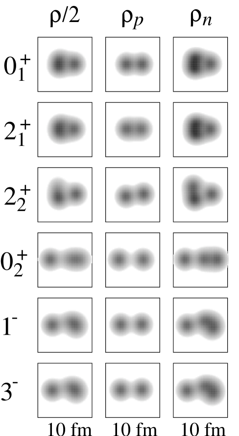
FIG. 30.: The intrinsic structure of the excited states of ¹⁰Be obtained by VAP calculations. The density distribution of matter, protons and neutrons of the intrinsic states are shown at left, middle and right, respectively. The density is integrated along the axis perpendicular to adequate planes. The figures are for the results with the interaction (g).

B Behavior of valence neutrons

Even though we did not assume the existence of any clusters in the model, we have found that the most of the intrinsic states of ¹⁰Be contain $2\alpha+2n$ structures. We study the behavior of the valence neutrons surrounding $2\alpha$ by analyzing the single-particle wave functions to understand the role of the valence neutrons in the neutron-rich Be nuclei. Considering that an intrinsic state is approximately written by a Slater determinant $\Phi_{AMD}$, the single-particle wave functions and the single-particle energies of an intrinsic state are determined by diagonalizing the single-particle Hamiltonian which has been already explained in IV B 4.

The single-particle energies in the $0^{+}_{1}$, $1^{-}$ and $0^{+}_{2}$ states are shown in Fig. 31. In each state four neutron orbits from the bottom correspond to those for the neutrons in the $2\alpha$ clusters. The level spacing of these four lower orbits becomes smaller in $1^{-}$ than in $0^{+}_{1}$ and smallest in the $0^{+}_{2}$ state with the increase of the distance between clusters. We consider the last two neutrons in the higher orbits as the valence neutrons surrounding 2$\alpha$ cores. We display the density distributions of the single-particle wave functions for the two valence neutrons in the left column of Fig. 32. Figures in the middle and right columns of Fig. 32 are for the normalized density of the positive and the negative parity components projected from the single-particle wave functions, respectively. By analyzing the single-particle wave functions it is found that two valence neutrons of the $0^{+}_{1}$ states contain the negative parity components more than $80\%$ (the right column in figure 32) which seem to be $\pi$ bonds(Fig. 33(a)) in terms of molecular orbits. On the other hands in the case of $0^{+}_{2}$ band, the last 2 neutrons are predominantly in the positive parity orbits, which are analogous to the $\sigma$ bonds (Fig. 33 (b)). In the $1^{-}$ band, each valence neutron contains both the positive parity component like $\sigma$ and the negative parity one similar to $\pi$. Since the parity of the total system is negative in the $1^{-}$ band, the states are considered to have one neutron in $\sigma$ orbit and the other neutron in $\pi$ orbit after the parity projection. Therefore roughly speaking, the $0^{+}_{1}$, $1^{-}$ and $0^{+}_{2}$ states are understood as $2\alpha$ and two valence neutrons in $\pi^{2}$, $\sigma\pi$ and $\sigma^{2}$ orbits, respectively. The interesting point is that the valence neutrons play important roles to develop the clustering structure in the excited bands. We can argue that the clustering develops in the $1^{-}$ band and mostly in $0^{+}_{2}$ band owing to the $\sigma$ orbits of the valence neutrons, because the $\sigma$ orbit prefers the prolately deformed system as to gain its kinetic energy. This idea originates from the application of the two centers shell model to the $2\alpha$ dimer model of Be isotopes by W. von Oertzen [61] and consistent with the argument in the work with the method of AMD+HF by Doté et al. [37].

From the view points of the shell model, the levels $J^{\pi}=$$0^{+}_{1}$, $2^{+}_{1}$, $4^{+}_{1}$ in the $K^{\pi}=0^{+}_{1}$ band and $2^{+}_{2}$, $3^{+}_{1}$ in the $K^{\pi}=2^{+}_{1}$ are the $0\hbar\omega$ states. These states are dominated by the components with the same [442] spatial symmetry in the supermultiplet limit. On the other hands, the negative parity states in the $K^{\pi}=1^{-}$ are dominated by the $1\hbar\omega$ configurations as for the neutron $p$-shell. In the excited states in the $K^{\pi}=0^{+}_{2}$ band, the $2\hbar\omega$ configurations with 2 neutrons excited are prime. It is consistent with the rotational band seen in the $2\hbar\omega$ states of shell model calculations [55]. However the well-developed clustering structures in the $K^{\pi}=1^{-}$ and the $K^{\pi}=0^{+}_{2}$ bands contain considerably the higher configurations which are not included explicitly in the wavefunction of the $1\hbar\omega$ model space and $(0+2)\hbar\omega$ model space of the shell model. Also in the Skyrme Hartree-Fock calculations [57], the $0^{+}_{2}$ state is found to be a state with 2 neutrons in $sd$-orbits.

FIG. 31.: Single-particle energies in the intrinsic systems of the $0^{+}_{1}$, $1^{-}$ and $0^{+}_{2}$ states. The energies of protons(neutrons) are displayed in the left(right) side in each figure.

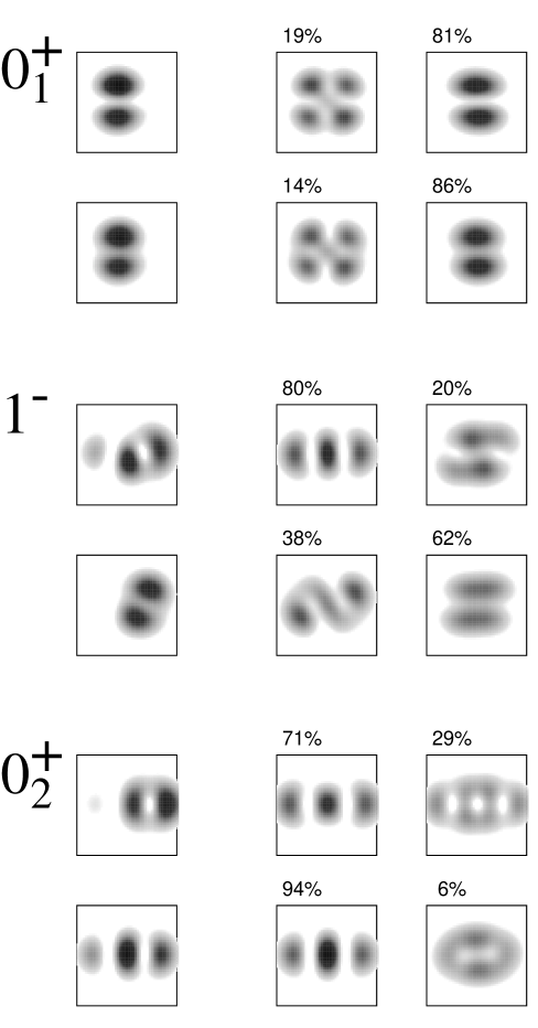
FIG. 32.: Density distribution of single-particle wave functions of the valence two neutrons in the intrinsic states of $0^{+}_{1}$, $1^{-}$ and $0^{+}_{2}$ (left column). The method to extract the single-particle wave functions are explained in the text. The middle and right columns are for the density of the positive parity and negative parity components projected from the single-particle wave functions, respectively. The wave functions projected into the parity eigen states are normalized in the presentation.

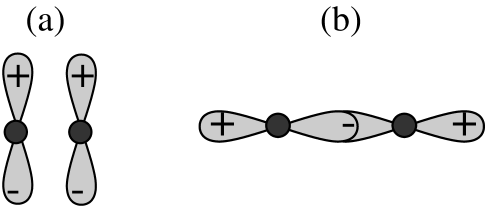
FIG. 33.: Schematic figures of the molecular orbits $\pi$ bond (a) and $\sigma$ bond (b) surrounding 2$\alpha$ clusters.

C Results of ¹²Be

In ¹²Be, one of the interesting problem is the vanishing of the magic number $N=8$ which is closely related with the abnormal parity of the ground state of the ¹¹Be. Another subject on ¹²Be is the molecule-like structure in the excited states which is reported in Ref. [28].

In present calculations, we adopt the interaction (h) with which we can reproduce the spin parity of the ground state 1/2⁺ of ¹¹Be. For comparison, we also use the interaction (g) which contains the weaker spin-orbit force than the interaction (h) and fails to reproduce the parity inversion in ¹¹Be. In the theoretical results of the energy levels we found many rotational bands such as $K^{\pi}=0^{+}_{1}$, $K^{\pi}=1^{-}_{1}$ and $K^{\pi}=0^{+}_{2}$. We present the density distributions of the intrinsic structures in Fig.34 for the results with the interaction (g). It is surprising that the intrinsic state of the ground band $K^{\pi}=0^{+}_{1}$ is the largely deformed molecule-like state with the dominant 2p-2h state in terms of neutron $p$-shell which is analogous to the second $0^{+}$ state in ¹⁰Be, while the second band $K^{\pi}=0^{+}_{2}$ is dominated by the normal $0\hbar\omega$ state with the rather spherical shape due to the neutron closed shell. It means the abnormal phenomena that the $sd$-orbits energetically intrude in the $p$-orbits and the magic number of $N=8$ vanishes in the ¹²Be. On the other hands, adopting the interaction (g) we obtain the rather spherical ground state with the closed neutron $p$-shell, and the deformed structure with 2p-2h appears in the second $0^{+}$ state lying a few MeV above the ground state. Such a difference in results between the adopted interactions (g) and (h) originates from the strength of spin-orbit force. The stronger spin-orbit force in (h) prefers the closed $p_{3/2}$-shell and breaks the $p$-shell in Be isotopes. With both interaction (g) and (h) we find the $K^{\pi}=1^{-}$ band with the developed clustering structure in the low-lying levels. The $K^{\pi}=0^{+}$ band with the 2p-2h configurations reaches to the $J^{\pi}=8^{+}$ state, and the band terminal of $K^{\pi}=1^{-}$ is found to be a $J^{\pi}=6^{-}$ state. The spins $8^{+}$ and $6^{-}$ at the band terminal are the same as the the highest spins in the corresponding configurations $(0p)^{2}_{\pi}(0p)^{4}_{\nu}(0d1s)^{2}_{\nu}$ and $(0p)^{2}_{\pi}(0p)^{5}_{\nu}(0d1s)^{1}_{\nu}$, respectively.

FIG. 34.: The intrinsic structure of the excited states of ¹²Be obtained by VAP calculations with the interaction (h). The density distribution of matter, protons and neutrons of the intrinsic states are shown at left, middle and right, respectively.

The $2\alpha+4n$ clustering structures are seen in many levels in ¹²Be. By analyzing the single-particle wave functions of the intrinsic structures in similar way to ¹⁰Be, we can roughly consider the $0^{+}_{1}$,$1^{-}$, and $0^{+}_{2}$ states as the state with 4 neutrons in $\pi^{2}\sigma^{2}$, $\pi^{3}\sigma^{1}$ and $\pi^{4}$ orbits surrounding $2\alpha$ in terms of the molecular-orbits $\pi$ and $\sigma$ for the valence neutrons. The clustering develops as the number of the valence neutrons in the $\sigma$ orbit increases.

The experimental value for Gamow-Teller transition strength $B(GT)$ from the ¹²Be ground state to the ¹²B ground state is 0.59 [60] deduced from experimental data of $\beta$ decay. The weaker GT decay from ¹²Be than expected with the shell-model calculations in the $0p$-shell model space has been discussed in the relations with the possible abnormal structure of the ground state [62]. The experimental $B(GT)$ value is the useful probe to investigate the structure of the ¹²Be ground state. One possible reason for the weak decay is considered to be that the ¹²Be ground state has more intruder admixture of the higher shell orbits. However there was no microscopic calculation which can describe the weak decay. To evaluate the $B(GT)$ we obtain the wave function for the final state by performing VAP calculations of ¹²B with $(J^{\pi},K^{\prime})=(1^{+},-1)$. The calculated $B(GT)$ with the interaction (h) is 0.8 which well agrees to the experimental data 0.59. Before the diagonalization for the obtained states, the GT strength from the $0^{+}_{1}$ state with large $2\hbar\omega$ components is 0.2, and that from the $0^{+}_{2}$ state with $0\hbar\omega$ is 3.0. The reason for the former value is that the state with $2\bar{\omega}$ configurations is forbidden to decay to the ¹¹B ground state which is almost the normal $0\hbar\omega$ state. The latter value is as much as the simple shell-model calculation and is much larger than the experimental data. After the diagonalization for the spin-parity eigen states projected from the obtained intrinsic states, the $0^{+}_{1}$ state and the $0^{+}_{2}$ state are mixed to redistribute the decay strength for the $0\hbar\omega$ state into other states. As a result, $B(GT)$ for ¹²Be($0^{+}_{1}$)$\rightarrow$¹²B($1^{+}$) is 0.8 and the one for ¹²Be($0^{+}_{2}$)$\rightarrow$¹²B($1^{+}$) is 2.1. Is it found that the main reason for the weak Gamow-Teller transition is that the ¹²Be ground state is dominated by the abnormal state with 2$\hbar\omega$ configurations. On the other hands, the calculations with the interaction (g) give much larger $B(GT)$ strength for ¹²B($0^{+}_{1}$)$\rightarrow$¹²B($1^{+}$) than the experimental data because in this case the main component of the ground state of ¹²Be is the $0\hbar\omega$ state.

The abnormal $2p-2h$ structure of the ground band of ¹²Be may be observed in the strength of $E2$ transitions. By using the interaction (h) which give the abnormal state for the ground band of ¹²Be, the $E2$ transition strength in the second band $B(E2;2^{+}_{2}\rightarrow 0^{+}_{2})$ is as small as the simple AMD calculations, however the $E2$ strength in the ground band $B(E2;2^{+}_{1}\rightarrow 0^{+}_{1})$ is predicted to be almost twice as large as the simple AMD result.

VI Mechanism of the developments of clustering structure in Be isotopes

In the study with the simplest version of AMD and with the VAP calculations, it is found that 2$\alpha$-cluster cores are seen in most of the low energy states of Be isotopes heavier than ⁷Be. In this section, we try to understand the mechanism of the clustering developments in Be isotopes systematically. We discuss this problem from two view points. First we take care of the valence neutrons in the molecular orbits. In the second subsection we give the discussion from the other view point of the two-center clusters.

A Molecular orbits of valence neutrons

In the study of Be isotopes with the simplest version of AMD, we have already shown the dependence of the development of the clustering structure on the neutron number (Fig. 17). We have discussed the clustering of the lowest states of the normal parity states with $0\hbar\omega$ configurations and the non-normal parity states with $1\hbar\omega$. In the study of the excited states with VAP calculations in the framework of AMD, we have found the rotational bands. The interesting point is that the rotaional bands can be classified by the number of the neutrons in the $sd$ orbits.

As already mentioned in the subsection V A, in the case of ¹⁰Be, three kinds of the intrinsic states construct the rotational bands. The intrinsic states are characterized by the orbits of the two valence neutrons surrounding $2\alpha$ cores. The lowest positive parity state in the $K=0^{+}_{1}$ band corresponds to the state with 2 neutrons in $p$-orbits. On the other hands, one neutron occupies the $sd$-orbit in the excited states in th $K=1^{-}_{1}$ band. Furthermore the states with two neutrons in the $sd$-orbits appear in the second $K=0^{+}_{2}$ band. The clustering develops larger and larger from $K=0^{+}_{1}$ to $K=1^{-}_{1}$ and to $K=0^{+}_{2}$.

According to the VAP calculations, we found these three kinds of the intrinsic states with $2\alpha$ cluster cores in the other neutron-rich nuclei ¹¹Be and ¹²Be as well as ¹⁰Be . Namely the most of the excited states in the low-energy region are classified into the states with the all the valence neutrons in the $p$-orbits, the states with one neutron in $sd$-orbit, and the states with two neutrons in $sd$-orbits which surround the $2\alpha$ cores. Strictly speaking the single-particle motion of the valence neutrons surrounding $2\alpha$ is not necessarily the ideal independent one but also the correlation between neutrons should be important. However, we think it useful to discuss the structure of Be isotopes from the viewpoints of molecule-like orbits surrounding $2\alpha$ because the component that neutrons occupy the molecule-orbits is significant in the neutron-rich Be isotopes

Here we improve the figure 17 for the development of the clustering in Be isotopes from the view points of the orbits of the valence neutrons surrounding $2\alpha$ cores. The Fig.35 presents the schematic figure for the cluster development of the lowest states in the given configurations. The lower line is for the state with all the valence neutrons surrounding $2\alpha$ in the $p$-orbits. The middle and upper lines correspond to the state with the one neutron and two neutrons in the $sd$-orbits, respectively. With the help of the figure 35 we can understand the development of the clustering in the Be isotopes systematically.

In the states with the same number of the valence neutrons in $sd$-orbits, the clustering development decreases gradually with the increase of the neutron number. The mechanism of the clustering development is easily understood by the idea of molecule-like orbits surrounding $2\alpha$ cores. In Be isotopes, the single particle wave functions of the the valence neutrons surrounding $2\alpha$ cores are analogous to the molecule-like orbits, $\pi$ and $\sigma$ orbits, which correspond to the $p$-orbit and $sd$-orbit in terms of the shell-model respectively, as shown in the subsection V A. In that sense the additional neutrons in each lines occupy the $\pi$-orbit as the neutron number increases. Therefore it seems that the valence neutrons in the $\pi$-orbits effect as to weaken the spatial clustering.

In the each Be nuclei, as the number of the neutrons in $sd$ orbits increases the clustering develops larger and larger. In the case of Be isotopes, the $sd$ orbits correspond to the $\sigma$ orbits. It is naturally understood that the valence neutrons in $\sigma$ orbits prefer the developed clustering states so as to gain the their kinetic energy. That is why the clustering develops as the increase of the number of neutrons in the $\sigma$ orbits.

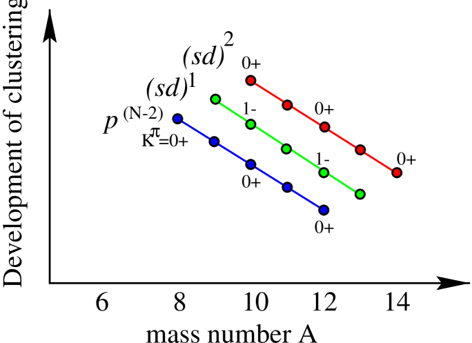
FIG. 35.: The schematic figure for the development of clustering in Be isotopes. The lines correspond to the cluster development of the lowest states in the given configurations (all the valence neutrons in the $p$-orbits, one neutron in the $sd$-orbits, and two neutrons in the $sd$-orbits) as the function of the mass number. The intrinsic states of the lowest states well correspond to the ones in the rotational bands.

B Viewpoint of the di-cluster structure

As mentioned above, one of the viewpoints for the mechanism of the clustering development is the explanation with the molecule-like orbits $\sigma$ and $\pi$. Here we try to understand the clustering in the excited states of ¹⁰Be from the other viewpoint of the two-center clustering model.

The reason for the clustering development in the ordinary nuclei has been considered as the system gains the kinetic energy with the development of clustering even if the potential energy looses. In order to understand the mechanism of clustering in light unstable nuclei, we think it helpful to investigate the competition of the kinetic and the potential energies in the molecule-like states of ¹⁰Be.

In the density distribution of VAP results, the structures of the $0^{+}_{1}$, $1^{-}$ and $0^{+}_{2}$ states seem to be the two-center clustering structures which consist of ⁶He+$\alpha$ (see figure 36). To estimate the dependence of the kinetic and potential energies on the degree of the spatial clustering development we represent the three kinds of configurations for the ⁶He+$\alpha$ system corresponding to the $0^{+}_{1}$, $1^{-}$ and $0^{+}_{2}$ states of ¹⁰Be by the simplified AMD wave functions $\Phi_{AMD}({\bf Z})$ as follows. The intrinsic spins of the single-particle wave functions are fixed to be up or down for simplicity. For the ⁶He+$\alpha$ system with the inter-cluster distance $d$ (fm), the centers of single-particle Gaussian wave functions are located around two points $\vec{a}_{1}=(-3d/5\sqrt{\nu},0,0)$ and $\vec{a}_{2}=(2d/5\sqrt{\nu},0,0)$. The three kinds of configurations of the centers for $0^{+}_{1}$, $1^{-}$ and $0^{+}_{2}$ states are shown in the right figures of Fig. 36. We put the centers for $p\uparrow$, $p\downarrow$, $n\uparrow$, $n\downarrow$ at the point $\vec{a}_{1}$ and $p\uparrow$, $p\downarrow$ at $\vec{a}_{2}$. The centers for the last 4 neutrons are located at the points very close to $\vec{a}_{2}$ as $\vec{a}_{2}\pm\vec{\delta}$ where enough small $\vec{\delta}$ is chosen so that the angle $\theta$ between $\vec{\delta}$ and $\vec{a}_{2}$ is $\theta$= $\pi/2$, $\pi/4$ and $0$ corresponding to the $0^{+}_{1}$, $1^{-}$ and $0^{+}_{2}$ states, respectively. For the parity eigen states projected from these three kinds of the simplified AMD wave functions $\Phi_{AMD}({\bf Z})$ we calculate the expectation values of total, kinetic and potential energies as the function of the inter-cluster distance $d$;

$$\langle H\rangle\equiv{\langle(1\pm P)\Phi_{AMD}({\bf Z})|H|(1\pm P)\Phi_{AMD}({\bf Z})\rangle\over\langle(1\pm P)\Phi_{AMD}({\bf Z})|(1\pm P)\Phi_{AMD}({\bf Z})\rangle}$$ (45)

$$\langle T\rangle\equiv{\langle(1\pm P)\Phi_{AMD}({\bf Z})|T|(1\pm P)\Phi_{AMD}({\bf Z})\rangle\over\langle(1\pm P)\Phi_{AMD}({\bf Z})|(1\pm P)\Phi_{AMD}({\bf Z})\rangle}$$ (46)

$$\langle V\rangle\equiv{\langle(1\pm P)\Phi_{AMD}({\bf Z})|V|(1\pm P)\Phi_{AMD}({\bf Z})\rangle\over\langle(1\pm P)\Phi_{AMD}({\bf Z})|(1\pm P)\Phi_{AMD}({\bf Z})\rangle},$$ (47)

where we omit the spin-orbit and the Coulomb forces for simplicity. In Fig. 37 we present the total energy, the kinetic energy and the potential energy for the three kinds of clustering states $0^{+}_{1}$, $1^{-}$ and $0^{+}_{2}$ as the function of the distance $d$ between ⁶He and $\alpha$ clusters. As shown in the figure for the total energy $\langle H\rangle$, the optimum distances indicate that the clustering structure develops in the system for the $1^{-}$ state and is most remarkable in the state for $0^{+}_{2}$, which is consistent with the present results of VAP calculations. The shift of the minimum point of the total energy is understood by the energetically advantage of the kinetic part as follows. It is found that the kinetic energies in the small $d$ region are sensitive to the configurations, while in the case of the potential energies significant differences are not seen in the three configurations. When the cluster approaches each other, the kinetic energy in the configuration for the $1^{-}$ state becomes larger than $0^{+}_{1}$ by ${1\over 2}\hbar\omega$ (about 7 MeV for $\nu=0.17$) because all the neutrons in $0^{+}_{1}$ are in $0s$ and $0p$ shells. On the other hands, in the negative parity state for $1^{-}$ one valence neutron must rise to the higher $sd$ shell in the small $d$ region. Since in the small $d$ limit the wave function is almost same as the harmonic oscillator shell model wave function due to the antisymmetrization, the kinetic energy of the $sd$ shell is larger by $1/2\hbar\omega$ than the one of $p$ shell. Thus the system for $1^{-}$ loses the kinetic energy in the small distance $d$, as a result, the minimum point of total energy shifts to the larger $d$ region than the one in the $0^{+}_{1}$ state. In the case of the linear configuration for the excited $0^{+}_{2}$ state, the two valence neutrons occupy the $sd$ orbit in the small $d$ limit and the kinetic energy is larger than $0^{+}_{1}$ by $\hbar\omega$. That is why the optimum point $d$ in $0^{+}_{2}$ is the largest of the three. In other words, when the cluster approaches each other, the system feels the repulsive force in kinetic part because of the Pauli principle. That is the reason why the clustering structure remarkably develops in the $0^{+}_{2}$ state. In the analysis with this simplified two cluster model, we can conclude that the clustering develops so as to gain the kinetic energy. It is compatible with the viewpoint of the molecular $\sigma$ orbit.

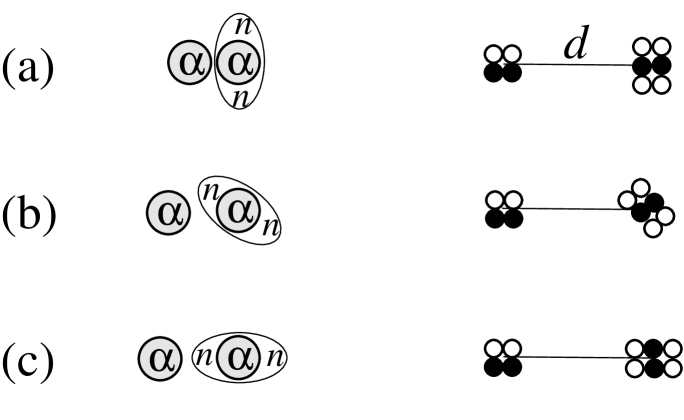
FIG. 36.: Schematic figures for the intrinsic structure of $0^{+}_{1}$, $1^{-}$ and $0^{+}_{2}$ from the view point of the two-center cluster model are shown in the left columns of (a), (b) and (c), respectively. In the right columns we display three kinds of the configurations of the centers of Gaussians in the simplified AMD wavefunctions which indicate the two-center ⁶He+$\alpha$ cluster model for the excited states $0^{+}_{1}$(a), $1^{-}$(b) and $0^{+}_{2}$(c) of ¹⁰Be. The black(white) circles correspond to the centers of Gaussians of the single-particle wave functions of protons(neutrons).

FIG. 37.: Total, kinetic and potential energies as functions of the distance between clusters in the simplified ⁶He+$\alpha$ cluster models for the excited states of ¹⁰Be. The adopted interaction is the MV1 force with $m=0.62$, and the spin-orbit and the Coulomb forces are omitted. The distance $d$ between clusters and the configuration for the $0^{+}_{1}$, $1^{-}$ and $0^{+}_{2}$ states are defined in the text. The solid lines, the dashed lines and the dot-dashed lines correspond to the energies in the system for $0^{+}_{1}$, $1^{-}$ and $0^{+}_{2}$ states of ¹⁰Be, respectively. It is found that the minimum point shifts outward from $0^{+}_{1}$ to $0^{+}_{2}$ because of the repulsive kinetic force in the small $r$ region.

VII Summary

We studied the structures of the ground and the excited states of light unstable nuclei with the theoretical method of AMD.

Li, Be, B and C isotopes were investigated with the simplest version of AMD. We showed the calculated results of binding energies, energy levels, radii, magnetic moments, electric moments, and transition strengths comparing with the experimental data. The AMD calculations systematically reproduce a lot of experimental data of many nuclei. By analyzing the intrinsic wave functions, we found the drastic changes between shell-model-like structures and clustering structures. The theoretical results suggest some new features in unstable nuclei such as the clustering structures, the molecular orbits, the opposite deformation between protons and neutrons, the neutron skin structures, et al. We discussed these phenomena with the help of the experimental informations.

We adopted VAP calculations to study the excited states of neutron-rich Be isotopes. Many excited levels were reproduced and were predicted by theory. We showed the theoretical results of the $E1$, $E2$, and $\beta$ transition strength, which agree well with the experimental data. By analyzing the structures of excited states in ¹⁰Be and ¹²Be, rotational bands $K^{\pi}=0^{+}_{1}$, $1^{-}$, $0^{+}_{2}$ are found. Particularly $K^{\pi}=1^{-}$ and $0^{+}_{2}$ bands have the largely deformed states with the molecule-like structures which consist of the developed $2\alpha$ clusters and surrounding neutrons. We extracted the single-particle wave functions to discuss the behavior of the valence neutrons, and found that the valence neutrons in molecule-like orbits surrounding $2\alpha$ play important roles in the clustering structure.

In order to understand the mechanism of the clustering development, we discussed the clustering structures of Be isotopes from two view points, the view point of the molecular orbits of the valence neutrons and the one of the two-center cluster model. We concluded that the clustering development in neutron-rich nuclei can be understood by the roles of the excess neutrons.

Although AMD calculations describe many new phenomena seen in unstable nuclei, however, future problems remain to be solved. For example, the extremely large radii due to the neutron halo structures are not reproduced because the AMD wave functions written by Gaussians are not enough to represent the long tail of the single particle wave functions. It is not obvious which the effective interaction parameters should be adopted in AMD framework. We must more carefully check the properties of the effective interactions such as the spin-orbit force and the central force. At least when the study goes to the heavier nuclear systems, we will soon meet the problems of the saturation property. That is to say that it is difficult to reproduce all the binding energies of the stable nuclei in the wide mass-number region with a set of parameters of the adopted interactions in the present work. Owing to the progress of the computational power, it becomes possible to make AMD calculations for the heavier unstable nuclei, where we may discover the other exotic structures such as the polymers of $\alpha$ clusters and the super deformations.

Finally we stress again that, as far as we know, the present work is the first theoretical study which can systematically describe the various clustering structures and shell-model-like structures in the ground and the excited states of many light unstable nuclei in one framework without assuming any inert cores nor the existence of clusters.

The computational calculations of this work were partially supported by the Research Center for Nuclear Physics in Osaka University. We owe the calculations to the system in Yukawa Institute for Theoretical Physics in Kyoto University, and the super computer systems in High Energy Accelerator Research and in the Institute of Physical and Chemical Research.

REFERENCES

- [1] Proc. VI Int. Conf. on Nuclei Far from Stability and IX Int. Conf. on Atomic Masses and Fundamental Constants, Bernkastel-Kues (1992), eds. R. Neugart and A. Wöhr, Institute of Physics Conference Series No. 132 (1993).
- [2] Proc. II Int. Conf. on Radioactive Nuclear Beams, Louvain-la Neuve (1991), ed. Th Delbar (IOP Publishing, London, 1992).
- [3] Proc. IV Int. Conf. on Nucleus-Nucleus Collisions , Kanazawa (1991), eds. H. Toki, I. Tanihata, and H. Kamitsubo, Nucl. Phys. A538 ( North Holland, 1992 ).
- [4] Proc. Int. Symp. on Structure and Reactions of Unstable Nuclei, Niigata (1991), eds. K. Ikeda and Y. Suzuki, ( World Scientific, 1992 ).
- [5] I. Tanihata, H. Hamagaki, O. Hashimoto, S. Nagamiya, Y. Shida, N. Yoshikawa, O. Yamakawa, K. Sugimoto, T. Kobayashi, D. E. Greiner, N. Takahashi, and Y. Nojiri, Phys. Lett. B160, 380 (1985); I. Tanihata, H. Hamagaki, O. Hashimoto, Y. Shida, N. Yoshikawa, K. Sugimoto, O. Yamakawa, T. Kobayashi, and N. Takahashi, Phys. Rev. Lett. 55, 2676 (1985); I. Tanihata, T. Kobayashi, O. Yamakawa, S. Shimoura, K. Ekuni, K. Sugimoto, N. Takahashi, T. Shimoda, and H. Sato, Phys. Lett. B206, 592 (1988), and references therein.
- [6] W. Mittig, J. M. Chouvel, Zhang Wen Long, L. Bianchi, A. Cunsolo, B. Fernandez, A. Foti, J. Gastebois, A. Gillebert, C. Gregoire, Y. Schutz, and C. Stephan, Phys. Rev. Lett. 59, 1889 (1987); M. G. Saint-Laurent, R. Anne, D. Bazin, D. Guillemaud-Mueller, U. Jahnke, Jin Gen Ming, A. C. Mueller, J. F. Bruandet, F. Glasser, S. Kox, E. Liatard, Tsan Ung Chan, G. J. Costa, C. Heitz, Y. El-Masri, F. Hanappe, R. Bimbot, E. Arnold, and R. Neugart, Z. Phys. A332, 457 (1989).
- [7] T. Kobayashi, O. Yamakawa, K. Omata, K. Sugimoto, T. Shimoda, N. Takahashi, and I. Tanihata, Phys. Rev. Lett. 60, 2599 (1988); R. Anne, S. E. Arnell, R. Bimbot, H. Emling, D. Guillemaud-Mueller, P. G. Hansen, L. Johannsen, B. Jonson, M. Lewitowitz, S. Mattsson, A. C. Mueller, R. Neugart, G. Nyman, F. Pougheon, A. Richter, K. Riisager, M. G. Saint-Laurent, G. Schrieder, O. Sorlin, and K. Wilhelmsen, Phys. Lett. B250, 19 (1990); M. Fukuda, T. Ichihara, N. Inabe, T. Kubo, H. Kumagai, T. Nakagawa, Y. Yano, I. Tanihata, M. Adachi, K. Asahi, M. Kouguchi, M. Ishihara, H. Sagawa, and S. Shimoura, Phys. Lett. B268, 339 (1991).
- [8] E. Arnold, J. Bonn, R. Gegenwart, W. Neu, R. Neugart, E.-W. Otten, G. Ulm, K. Wendt, and ISOLDE Collaboration, Phys. Lett. B197, 311 (1987).
- [9] E. Arnold, J. Bonn, W. Neu, R. Neugart, E.W. Otten, the ISOLDE Collaboration, Z. Phys. A331, 295 (1988); E. Arnold, J. Bonn, A. Klein, R. Neugart, M. Neuroth, E.W. Otten, P. Lievens, H. Reich, W. Widdra, and ISOLDE Collaboration, Phys. Lett. B281, 16 (1992).
- [10] H. Okuno, K. Asahi, H. Ueno, H. Sato, M. Adachi, T. Kubo, T. Nakamura, N. Inabe, A. Yoshida, Y. Ohkubo, T. Ichihara, M. Ishihara, T. Shimoda, H. Miyatake, and N. Takahashi, Hyperfine Interactions 78, 97 (1993).; K. Asahi, H. Ueno, H. Izumi, H. Okuno, K. Nagata, H. Ogawa, Y. Hori, H. Sato, K. Mochinaga, M. Adachi, A. Yoshida, G. Liu, N. Aoi, T. Kubo, M. Ishihara, W.-D. Schmidt-Ott, T. Shimoda, H. Miyatake, S. Mitsuoka, and N. Takahashi, to appear in Proc. Int. Symp. on Physics of Unstable Nuclei, Niigata(1994), eds. H. Horiuchi, K. Ikeda, K. Sato, Y. Suzuki, and I. Tanihata, Nucl. Phys. A (1995).
- [11] H. Okuno and K. Asahi, private communication.
- [12] K.Matsuta, M. Fukuda, M. Tanigaki, T. Minamizono, Y. Nojiri, M. Mihara, T. Onishi, T. Yamaguchi, A. Harada, M. Sasaki, T. Miyake, S. Fukuda, K. Yoshida, A. Ozawa, T. Kobayashi, I. Tanihata, J. R. Alonso, G. F. Krebs and T. J. M. Symons, Proc. Int. Symp. on Physics of Unstable Nuclei, Niigata(1994), eds. H. Horiuchi, K. Ikeda, K. Sato, Y. Suzuki, and I. Tanihata, Nucl. Phys. A 153c(1995).
- [13] D. Bazin, B.A. Brown, J. Brown, M.Fauerbach, M. Hellstrom, S.E. Hirzebruch, J.H. Kelley, R.A. Kryger, D.J. Morrissey, R. Pfaff, C.F. Powell, B.M. Sherrill and M. Thoennessen, Phys. Rev. Lett. bf 74 3569 (1995).
- [14] M. V. Zhukov, B. V. Danilin, D. V. Fedorov, J. M. Bang, I. J. Thompson, and J. S. Vaagen, Phys. Report 231, No.4, 151 (1993); K. Ikeda, Nucl. Phys. A538, 355c (1992).
- [15] A. A. Korsheninnikov, B. V. Danilin, and M. V. Zhukov, Nucl. Phys. A559, 208 (1993).
- [16] K. Varga, Y. Suzuki, and Y. Ohbayashi, Phys. Rev. C50, 189 (1994); K. Varga, Y. Suzuki, and R. Lovas, Nucl. Phys. A571, 447 (1994).
- [17] K. Varga, Y. Suzuki, and I. Tanihata, Proc. Int. Symp. on Physics of Unstable Nuclei, Niigata(1994), eds. H. Horiuchi, K. Ikeda, K. Sato, Y. Suzuki, and I. Tanihata, Nucl. Phys. A588 157c(1995). ; K. Varga, Y. Suzuki, and I. Tanihata, preprint RIKEN-AF-NP-179 (RIKEN, 1994).
- [18] Y. Ogawa, K. Arai, Y. Suzuki, and K. Varga, preprint RIKEN-AF-NP-291(1998)
- [19] N. Itagaki and S. Okabe, preprint RIKEN-AF-NP-314 (1999).
- [20] Y. Utsuno, T. Otsuka, T. Mizusaki and M. Honma, Phys.Rev.C60 054315 (1999)
- [21] N. Tajima, N. Onishi and S. Takahara, Proc. Int. Symp. on Physics of Unstable Nuclei, Niigata(1994), eds. H. Horiuchi, K. Ikeda, K. Sato, Y. Suzuki, and I. Tanihata, Nucl. Phys. A588 215c(1995).
- [22] M. Stoitsov, P. Ring, D. Vretenar and G.A. Lalazissis, Phys.Rev.C58 2086 (1998)
- [23] K. Ikeda, H. Horiuchi, S. Saito, Y. Fujiwara, M. Kamimura, K. Kato, Y. Suzuki, E. Uegaki, H. Furutani, H. Kanada, T. Kaneko, S. Nagata, H. Nishioka, S. Okabe, T. Sakuda, M. Seya, Y. Abe, Y. Kondo, T. Matsuse, and A. Tohsaki- Suzuki, Comprehensive Study of Structure of Light Nuclei, Prog. Theor. Phys. Suppl. 68, (1980).
- [24] A. Arima, Nuclear Cluster Correlation, Heavy Ion Collisions, Vol. 1, Chapt.3 , ed. R. Bock, ( North Holland, Amsterdam, 1979 ), p.417.
- [25] Y. C. Tang, Microscopic Description of the Nuclear Cluster Theory, Lecture Notes in Physics 145, ( Springer, Berlin, 1981 ).
- [26] V. I. Kukulin, V. G. Neudatchin, I. T. Obukhovski, and Yu. F. Smirnov, Clusters as Subsystems in Light Nuclei, ( Clustering Phenomena in Nuclei Vol.3, Vieweg, Braunschweig, 1982 ), p.1.
- [27] H. Horiuchi and K. Ikeda, Cluster Model of the Nucleus, International Review of Nuclear Physics Vol.4, eds. T. T. S. Kuo, and E. Osnes, (World Scientific, Singapore, 1985), pp.1 258.
- [28] M. Freer, et al., Phys. Rev. Lett. 82, 1383 (1999).
- [29] Y. Kanada-En’yo, A. Ono and H. Horiuchi, Phys. Rev. C 52, 628 (1995).
- [30] Y. Kanada-En’yo and H. Horiuchi, Phys. Rev. C 52, 647 (1995).
- [31] A. Ono, H. Horiuchi, T. Maruyama, and A. Ohnishi, Phys. Rev. Letters 68, 2898 (1992).
- [32] A. Ono, H. Horiuchi, T. Maruyama, and A. Ohnishi, Prog. Theor. Phys. 87, 1185 (1992).
- [33] A. Ono, H. Horiuchi, T. Maruyama, and A. Ohnishi, Phys. Rev. C47, 2652 (1993).
- [34] A. Ono, H. Horiuchi, and T. Maruyama, Phys. Rev. C48, 2946 (1993).
- [35] A. Ono and H. Horiuchi, Phys. Rev. C51, 299 (1995).
- [36] Y. Kanada-En’yo and H. Horiuchi, Prog. Theor. Phys. 93, 115 (1995).
- [37] A. Doté, H. Horiuchi, and Y. Kanada-En’yo, Phys. Rev. C 56, 1844 (1997).
- [38] Y. Kanada-En’yo, Phys. Rev. Lett. 81, 5291 (1998).
- [39] Y. Kanada-En’yo, H. Horiuchi and A. Doté Phys. Rev. C 64, 064304(1999)
- [40] A. B. Volkov, Nucl. Phys. 74, 33 (1965).
- [41] T. Ando, K.Ikeda, and A. Tohsaki, Prog. Theor. Phys. 64, 1608 (1980).
- [42] N. Yamaguchi, T. Kasahara, S. Nagata, and Y. Akaishi, Prog. Theor. Phys. 62, 1018 (1979); R. Tamagaki, Prog. Theor. Phys. 39, 91 (1968).
- [43] A. Ozawa et al., preprint RIKEN-AF-NP-294 (RIKEN, 1998) and references therein.
- [44] Y. Kanada-En’yo, Docter thesis (1996).
- [45] Y. Kanada-En’yo and H. Horiuchi, Phys. Rev. C 55, 2860 (1997).
- [46] P. Raghavan, At. Data Nucl. Data Tables 42, 189 (1989).
- [47] M. Seya, M. Kohno, and S. Nagata, Prog. Theor. Phys. 65, 204 (1981).
- [48] D. M. Brink, Proc. Int. School of Phys. ”Enrico Fermi”, course 36 (1965), ed. C. Bloch, p.247.
- [49] B. F. Bayman and A. Bohr, Nucl. Phys. 9, 596 (1958/59).
- [50] I. Tanihata et al., Phys.Lett. B289, 261 (1992)
- [51] O.V. Bochkarev et al., Eur.Phys.J. A 1, 15(1998).
- [52] T. Suzuki et al., Phys. Rev. Lett. bf 75 3241 (1995)
- [53] N. Fukunishi, T. Otsuka and I. Tanihata, preprint, RIKEN-AF-NP-153(RIKEN, 1993).
- [54] I. Daito, et al., Phys. Lett. B 418 27 (1998).
- [55] E. K. Warburton and B. A. Brown, Phys. Rev. C 46, 923(1992).
- [56] A. A. Wolters, A. G. M. van Hees, and P. W. M. Glaudemans, Phys. Rev. C 42, 2062 (1990).
- [57] S. Takami, K. Yabana, and K. Ikeda, Contribution paper to the International Symposium on Physics of Unstable Nuclei, Niigata (1994), Contribution Booklet C-34.
- [58] F. Ajzenberg-Selove, Nucl. Phys. A 490, 1 (1988).
- [59] H. Nakada and T. Otsuka, Phys. Rev. C 49, 886 (1994).
- [60] W. -T. Chou, E. K. Warburton and B. A. Brown, Phys. Rev. C 47, 163 (1993).
- [61] W. von Oertzen, preprint (1996).
- [62] T. Suzuki and T. Otsuka, Phys. Rev. bf C 56, 847(1997).