Effective boost and “point-form” approach

Abstract

Triangle Feynman diagrams can be considered as describing form factors of states bound by a zero-range interaction. These form factors are calculated for scalar particles and compared to point-form and non-relativistic results. By examining the expressions of the complete calculation in different frames, we obtain an effective boost transformation which can be compared to the relativistic kinematical one underlying the present point-form calculations, as well as to the Galilean boost. The analytic expressions obtained in this simple model allow a qualitative check of certain results obtained in similar studies. In particular, a mismatch is pointed out between recent practical applications of the point-form approach and the one originally proposed by Dirac.

The point-form calculation of form factors in impulse approximation has recently been performed for various systems: the deuteron KLIN0 , the nucleon WAGE and a bound state of two scalar particles interacting via the exchange of a massless scalar boson DESP0 . With respect to a non-relativistic calculation, discrepancies with experimental data are slightly increased in the first case and essentially removed in the second one. For the last case, there is no experiment but a more complete calculation in ladder approximation can be performed. Indeed, the Bethe-Salpeter equation BETH can then be solved easily, due to a hidden symmetry in the Wick-Cutkosky model WICK ; CUTK . Moreover, this model accounts for minimal features of realistic interaction models, such as the field-theory character or explicit relativistic covariance. For this system, the exact and point-form calculations of the form factors strongly differ DESP0 , especially when the zero-mass limit is approached or when large $Q^{2}$ are considered, two limits that a relativistic approach should be able to deal with. This test case points to an important contribution from two-body currents. Amazingly, a calculation using the non-relativistic expressions for the form factors with the point-form wave functions does rather well. The difference resides mainly in the expression of the transformed momenta under a boost. Unfortunately, the complexity of the calculation in the Wick-Cutkosky model prevents one from checking this point directly on the expression of the form factors.

However, there exists a simpler model which allows for a completely analytic solution and which therefore is particularly useful to gain insight into the origin of the above mentioned properties. This model describes a bound state of two scalar particles together with a zero-range interaction, providing another case where the Bethe-Salpeter equation may be solved in closed form. Contrary to the Wick-Cutkosky model however, the interaction now is of short range, which allows one to check qualitative features obtained in ref. DESP0 with a different interaction model. The fully covariant amplitude for the bound state of total mass $M^{2}=P^{2}$ in this case is given by:

$$\Phi(P,p)=\frac{C}{\left(m^{2}-p^{2}\right)\left(m^{2}-\big{(}P-p\big{)}^{2}\right)},$$ (1)

where $p$ is the four-momentum of one of the two constituents with equal mass $m$, and $C$ is a normalization constant.

This solution may be used to calculate form factors of the bound state in closed form. These form factors are represented by the triangle Feynman diagram shown in Fig. 1. Of particular interest in the present context is the expression obtained for the electromagnetic form factor after integrating over the zero component of the spectator particle four momentum. In the Breit frame it reads:

$$F_{1}(Q^{2})=\frac{C^{2}}{2}\int\frac{d\,\vec{p}}{(2\,\pi)^{3}}\;\frac{(e_{i}+e_{f}+2\,e_{p})}{e_{p}\,(e_{i}+e_{f})\,(E^{2}-(e_{i}+e_{p})^{2})\,(E^{2}-(e_{f}+e_{p})^{2})},$$ (2)

with $E=\sqrt{M^{2}+(\vec{Q}/2)^{2}}$, $e_{i}=\sqrt{m^{2}+(\vec{p}+\vec{Q}/2)^{2}}$, $e_{f}=\sqrt{m^{2}+(\vec{p}-\vec{Q}/2)^{2}}$ and $e_{p}=\sqrt{m^{2}+\vec{p}^{\;2}}$.

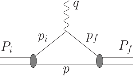
Figure 1: Representation of a virtual photon absorption on a two-body system with the kinematical definitions.

In this form it does not contain an obvious track of a bound state but this feature becomes apparent when looking at the expression at $q^{\mu}=0$:

$$F_{1}(0)=\frac{C^{2}}{2}\frac{1}{M}\,\int\frac{d\vec{k}}{(2\,\pi)^{3}}\left[\;\left(\frac{1}{2\,e_{k}\,(M-2\,e_{k})}\right)^{2}-\left(\frac{1}{2\,e_{k}\,(M+2\,e_{k})}\right)^{2}\right].$$ (3)

The dominant first term of this expression is precisely what we get for the norm of a system described by the wave function $\phi(\vec{k})=c/[2\,e_{k}\,(M-2\,e_{k})]$, which itself corresponds to a zero-range interaction in a semi-relativistic potential model. This wave function has the structure expected for a solution of the mass operator, $M=2\,e_{k}+V$ (in the c.m.). Therefore, we have another model where the point-form approach in impulse approximation can be checked reliably since the calculation of the Feynman diagram of Fig. 1 is straightforward.

Results for the elastic charge form factor in the point-form approach can be obtained from expressions given in ref. DESP0 :

$$F_{1}(Q^{2})=\frac{1+v^{2}}{\sqrt{1-v^{2}}}\int\frac{d\vec{p}}{(2\pi)^{3}}\;\phi_{f}(\vec{p}_{tf})\;\phi_{i}(\vec{p}_{ti}),$$ (4)

where the velocity $\vec{v}$ is related to the momentum transfer by the relation $v^{2}=Q^{2}/(Q^{2}+4M^{2})$ for the elastic case, and the Lorentz-transformed momenta are defined as: $(p^{x},p^{y},p^{z})_{tf}=(p^{x},p^{y},\frac{p^{z}-v\,e_{p}}{\sqrt{1-v^{2}}})$ and $(p^{x},p^{y},p^{z})_{ti}=(p^{x},p^{y},\frac{p^{z}+v\,e_{p}}{\sqrt{1-v^{2}}})$. A similar relation holds for the scalar form factor DESP2 .

Results of a non-relativistic calculation,

$$F_{1}(Q^{2})=\int\frac{d\vec{p}}{(2\pi)^{3}}\;\;\phi_{f}\Big{(}\vec{p}-\frac{1}{4}\vec{q}\,\Big{)}\;\;\phi_{i}\Big{(}\vec{p}+\frac{1}{4}\vec{q}\,\Big{)},$$ (5)

which implies the use of the same wave functions $\phi(\vec{p}\,)$ as previously quoted together with a Galilean boost, will also be considered. This is mainly done to emphasize the role of the different boost expressions, as discussed below, the relevance of a non-relativistic calculation being a priori questionable for the high momentum transfers (up to $Q^{2}=100\,m^{2}$) that we will consider.

Table 1: Elastic scalar- and vector- form factors, $F_{0}(q^{2})$ and $F_{1}(q^{2})$. Results are given successively for the Feynman diagram ($F.D.$) (identical to a Bethe-Salpeter calculation with a zero-range interaction), the point-form approach ($P.F.$) and the non-relativistic case ($N.R.$), and for two total masses.

$Q^{2}/m^{2}$	0.01	0.1	1.0	10.0	100.0
$M=1.6\,m$
$F_{0}\;\;\;\;F.D.$	1.325	1.309	1.176	0.659	0.187
$F_{1}\;\;\;\;F.D.$	0.999	0.989	0.908	0.566	0.191
$F_{0}\;\;\;\;P.F.$	0.511	0.499	0.393	0.095	0.33-02
$F_{1}\;\;\;\;P.F.$	0.998	0.989	0.904	0.485	0.82-01
$F_{0,1}\;\;N.R.$	0.998	0.991	0.923	0.595	0.210
$M=0.1\,m$
$F_{0}\;\;\;\;F.D.$	1.498	1.487	1.389	0.920	0.320
$F_{1}\;\;\;\;F.D.$	0.999	0.995	0.954	0.723	0.315
$F_{0}\;\;\;\;P.F.$	0.015	0.27-02	0.87-04	0.15-05	0.20-07
$F_{1}\;\;\;\;P.F.$	0.956	0.482	0.74-01	0.77-02	0.78-03
$F_{0,1}\;\;N.R.$	0.999	0.998	0.979	0.840	0.465

A sample of results is given in Table 1 for both a scalar and a vector (charge) form factor, and for two masses, $M=1.6\,m$ and an extreme relativistic case, $M=0.1\,m$. One notices that the point-form results fail to reproduce the exact ones, especially in the limit $M\rightarrow 0$ or for the scalar probe. They qualitatively confirm results obtained in ref. DESP0 , despite a significant difference in the interaction models: long-range in ref. DESP0 , short range in the present work. The fact that the non-relativistic calculation does well in all cases strongly suggests that the effective boost is closer to the non-relativistic than to the kinematical relativistic one. Some of the details may be discussed, but the size of the discrepancy is so large, especially when the total mass M goes to zero or $Q^{2}$ goes to $\infty$, that there is no doubt on the diagnostic. We remark that there also exist discrepancies for $F_{0}$ at low $Q^{2}$. They may be accounted for by two-body currents that have a close relationship to Z-type diagrams in an instant-form approach. They are not considered here since they are common to both the point-form and the non-relativistic calculations.

We shall now use the different expressions obtained above to directly compare the boost transformations applied in different approaches. This will provide further insight into the features evidenced by the results of Table 1 and those presented in refs. KLIN0 ; WAGE ; DESP0 . The transformed momenta, when a system of total mass $M$ is boosted to acquire a momentum $\vec{P}$ (equal to $\vec{q}/2$ in the Breit frame employed in Eqs. (4,5)), in the Galilean-covariant and the point-form approach, are respectively given by:

$$\vec{p}=\displaystyle\vec{k}+\displaystyle\frac{\vec{P}}{2}, ({\rm non-relativistic})$$ (6)

$$\displaystyle\vec{p}=\displaystyle\vec{k}+\displaystyle\frac{\vec{k}\cdot\vec{P}\;\,\vec{P}}{\vec{P}^{2}}\left(\sqrt{1+\vec{P}^{2}/M^{2}}\;\;-1\right)+\displaystyle\frac{\vec{P}}{2}\;\displaystyle\frac{2\sqrt{m^{2}+\vec{k}^{2}}}{M},\qquad ({\rm point-form})$$ (7)

where $\vec{p}$ and $\vec{k}$ are the momenta of the spectator particle in the moving and in the c.m. frames. A large part of the difference between non-relativistic and point-form results is due to the presence of the factor $2\sqrt{m^{2}+\vec{k}^{2}}/M$ multiplying $\vec{P}/2$ in Eq. (7). It tends to make the momentum transfer actually larger than what it should be, hence larger charge radii and faster fall-off of form factors as it is observed from results presented in refs. WAGE ; DESP0 . The fact that the non-relativistic calculation does relatively well suggests that this factor is effectively absent in the exact calculation of form factors.

A qualitative confirmation is obtained by the examination of Eq. (2), which indicates that the combination of the vectors $\vec{p}$ and $\vec{Q}/2$, that appears in many places, is the same as given by a Galilean boost, Eq. (6). This feature has a general character and it explains why a non-relativistic calculation of form factors is not so bad, contrary to what might be expected a priori. Similar results hold for the form factor relative to a scalar probe.

We first analyze the expression of the exact form factors, Eq. (2), at $q^{\mu}=0$. In this case, the calculation can be performed by integrating over the time component of the spectator particle, for the system at rest or with arbitrary momentum $\vec{P}$. As the result is a covariant one, it should be the same in any frame, thus providing a relation between the momenta of the spectator particle in the c.m. and in the moving system. The result is given by:

$$\vec{p}=\vec{k}+\frac{\vec{k}\cdot\vec{P}\;\,\vec{P}}{\vec{P}^{2}}\Big{(}\sqrt{1+\vec{P}^{2}/(4\,e_{k}^{2})}\;\;-1\Big{)}+\frac{\vec{P}}{2}.$$ (8)

This relation, which has been mentioned in a slightly different context in ref. HAMM , corresponds to an instant-form approach. Even though it does not exhibit an explicit dependence on the interaction, as it is the case for the transformation of Eq. (7), one has to remember that the relevant boost parameter is the velocity $\vec{v}/\sqrt{1-v^{2}}=\vec{P}/M$. Expressing Eqs. (7,8) in terms of this quantity shows the interaction and kinematics dependence of the boost in instant form and in point form, respectively, as it should be.

While Eq. (8) provides the desired result (absence of the factor $2\,e_{k}/M$ in front of $\vec{P}$), it is too early to conclude at this point. Indeed, other expressions of Eq. (2) can be obtained by performing the calculation of the Feynman triangle diagram, Fig. 1, in different ways. Instead of integrating over the time component of the four-momentum $p$, one can integrate over any linear combination of the four components, $\lambda\cdot p$, where $\lambda^{2}=1$. This would correspond to a description on a hyperplane $\lambda\cdot x=ct$. As the form factor is invariant under a Lorentz transformation and since the above change in the integration variable amounts to such a transformation with velocity $\vec{v}=\vec{\lambda}/\lambda_{0}$, a generalized relation immediately follows from Eq. (8):

$$\vec{p}=\vec{k}+\vec{\lambda}\,\left(\frac{\vec{k}\cdot\vec{\lambda}}{\lambda_{0}+1}+\frac{\vec{k}\cdot\vec{P^{\prime}}}{2\,e_{k}}\right)+\frac{\vec{k}\cdot\vec{P^{\prime}}\;\Big{(}\vec{P^{\prime}}+\vec{\lambda}\;\vec{\lambda}\cdot\vec{P^{\prime}}/(\lambda_{0}+1)\Big{)}}{4\,e_{k}^{2}\;\Big{(}1+\sqrt{1+\vec{P^{\prime}}^{2}/(4\,e_{k}^{2})}\;\Big{)}}+\frac{\vec{P}}{2}\;+\frac{\vec{\lambda}}{2}\;\left(\sqrt{4\,e_{k}^{2}+\vec{P^{\prime}}^{2}}-\sqrt{M^{2}+\vec{P^{\prime}}^{2}}\right),$$ (9)

where $\vec{P^{\prime}}$ is related to $\vec{P}$ by the Lorentz transformation:

$$\vec{P^{\prime}}=\vec{P}+\vec{\lambda}\,\frac{\vec{\lambda}\cdot\vec{P}}{\lambda_{0}+1}-\vec{\lambda}\,E_{P},$$ (10)

with $E_{P}=\sqrt{M^{2}+\vec{P}^{2}}$. For our purpose, only the two terms in Eq. (9) that do not vanish in the limit $\vec{k}\rightarrow 0$ are relevant. As it can be observed, the bracket in the very last term is proportional to $(2\,e_{k}-M)$. This factor corresponds to an effective interaction term and is characteristic of the contribution that appears here or there, depending on the relativistic approach. Thus, despite apparent differences, none of the expressions given by Eqs. (9,10) is favoured in calculating form factors, provided evidently that two-body currents originating from Z-type diagrams are included. In particular, it can be shown that Eq. (9) allows one to recover the relation used in point-form calculations, Eq. (7), by choosing $\lambda_{0}=E_{P}/M,\;\vec{\lambda}=\vec{P}/M$ (implying $\vec{P^{\prime}}=0$).

The above results can be extended to the case $q^{\mu}\neq 0$. While doing so, one has to take care that the initial and final states are described on the same surface, $\lambda\cdot x=ct$. Examining the recent point-form calculations, it is obvious that this condition is not fulfilled. The initial and final states are obtained from the state at rest, which is described on a surface $\lambda\cdot x=ct$, with $\lambda=(1,0,0,0)$. Applying a kinematical boost amounts to using a relation such as Eq. (9), with the appropriate $\lambda$. Thus, the states required for an estimate of form factors, in the Breit frame for instance, correspond to a description on two different surfaces, $\lambda\cdot x=ct$ with $(\lambda_{0},\;\vec{\lambda})=(1,\;-\vec{v})/\sqrt{1-v^{2}}$ for the initial state and $(\lambda_{0},\;\vec{\lambda})=(1,\;\vec{v})/\sqrt{1-v^{2}}$ for the final one. This is not the standard way of performing calculations that, generally, refer to one and the same definition of the surface on which quantization is performed, independently of the formalism used to implement relativity.

Having emphasized a possible mismatch in the description of initial and final states in the point-form calculations of form factors made up to now KLIN0 ; WAGE , we go back to the various expressions of the transformation of the momentum under a boost, Eqs. (6 – 9). From the above discussion, the relevant boost effect is determined by the relative boost of the initial and final states, both being described on the same surface, like the one given in Eq. (8). Taking into account that $\vec{P}$ is directly associated to the momentum transfer, one can anticipate that the effective enhancement of the momentum transfer due to the factor $2\,e_{k}/M$ in Eq. (7), which is responsible for the largest effect obtained in the point-form calculations of form factors, is essentially absent, as it can be checked on the full expression of the form factor of the system considered here. Unfortunately, an examination of Eq. (2) does not provide an effective boost transformation as it was the case before, however, it is clear that there do not arise any additional factors $2e_{k}/M$, suggesting that this effective boost is still closer to the non-relativistic than to the kinematical relativistic one.

In this paper, we considered another example where a comparison of a point-form calculation of form factors with an exact one is possible. It confirms earlier conclusions while providing analytical checks DESP0 . It is shown that the applications of the point-form approach made until now KLIN0 ; WAGE imply the description of the initial and final states on two different surfaces. This prevents one from considering time-ordered contributions (the invariant times for the two states are not defined in the same way). Interestingly, the effective boost that allows one to construct the final state from the initial one is closer to the non-relativistic than to the kinematical relativistic one, explaining the relative success of a non-relativistic description of form factors in a domain where it is not expected. Not surprisingly, the difference involves terms proportional to $2\,e_{k}-M$, which can be turned into an interaction term. The effective boost transformation accounts for a contribution originating from the free-particle energy, included in the present point-form calculation, but also one from the interaction term, which has to be accounted for separately in the point-form approach. When the system under consideration is given a velocity $\vec{v}$ (momentum $\vec{P}$), the two contributions are roughly given by $\simeq\vec{v}\,(2\,e_{k})/\sqrt{1-v^{2}}$ (which represents a contribution to the momentum enhanced by a factor $2\,e_{k}/M$) and $\simeq\vec{v}\,(M-2\,e_{k})/\sqrt{1-v^{2}}$ (which cancels this enhancement). We recall that this last term, whose corresponding contribution is obviously absent in the present point-form calculations of form factors, can be cast into an interaction term by using the expression of the mass operator, $2e_{k}+V=M$.

The failure of the currently applied point-form approach can be remedied by brute force, by adding two-body currents that are constructed such that they reproduce what is expected from Feynman diagrams once the one-body current is accounted for. One can hope to fulfill in this way current conservation and reproduce the Born amplitude, two constraints that are relevant at small and large momentum transfers, respectively. Some work along these lines is in progress DESP2 .

It is noticed that the present point-form calculations rely in practice on the use of wave functions obtained from quantization on a hyperplane $\lambda\cdot x=ct$. Originally, in Dirac’s work DIRA , this operation was supposed to be performed on a hyperboloïd, $x\cdot x=ct$. One can imagine that an approach fully consistent with this feature could remove some of the encountered problems. Despite a few attempts FUBI ; GROM , not much has been done along these lines however.

An intermediate approach, suggested by the above analysis, is to change the quantization surface for the initial or for the final state, or both, so that they coincide after a boost from the state at rest. This involves the dynamics, with the result that the original simplicity of the approach is lost. This procedure could be realized in an instant-form calculation, but the answer is not unique. However, starting from the Breit-frame results, covariant ones are obtained by the particular choice, $\lambda^{\mu}=(P_{i}+P_{f})^{\mu}/\sqrt{(P_{i}+P_{f})^{2}}$, the only one consistent with the symmetry between initial and final states. With this definition, the quantization surface, $\lambda\cdot x=ct$, is unchanged under a Lorentz transformation while it is modified in a standard instant-form calculation where $\lambda=(1,0,0,0)$.

This invariance is not equivalent to the one resulting from the consideration of a hyperboloïd surface. Nevertheless, by proceeding this way one recovers some of the properties expected in a full point-form calculation. From what we checked, the major problems evidenced by the present point-form calculations are removed. It has to be shown however, whether a fully consistent approach can be constructed along these lines.

Acknowledgements This work has been supported in part by the EC-IHP Network ESOP, contract HPRN-CT-2000-00130 and the DGESIC (Spain), under contract PB97-1401-C02-01.

References

- (1) T.W. Allen, W.H. Klink and W.N. Polyzou, Phys. Rev. C 63, 034002 (2001).
- (2) R. Wagenbrunn et al., Phys. Lett. B 511, 33 (2001) .
- (3) B. Desplanques and L. Theußl, nucl-th/0102060.
- (4) E.E. Salpeter and H.A. Bethe, Phys. Rev. 84, 1232 (1951).
- (5) G.C. Wick, Phys. Rev. 96, 1124 (1954).
- (6) R.E. Cutkosky, Phys. Rev. 96, 1135 (1954).
- (7) B. Desplanques and L. Theußl, in preparation.
- (8) B. Hamme and W. Glöckle, Few-Body Systems 13, 1 (1992).
- (9) P.A.M. Dirac, Rev. Mod. Phys. 21, 392 (1949).
- (10) S. Fubini, A.J. Hanson and R. Jackiw, Phys. Rev. 7, 1732 (1973).
- (11) D. Gromes, H. J. Rothe and B. Stech, Nucl. Phys. B75, 313 (1974).