Microscopic derivation of pion-nucleon and pion-Delta scattering lengths

Abstract

A general expression for the $\pi-N$ and $\pi-\Delta$ scattering lengths is derived in the framework of a microscopic calculation. Annihilation, negative energy wave-functions and spontaneous chiral symmetry are included consistently. The point-like limit is used to calculate the scattering lengths.

1 Introduction

In the last decade a global picture for low energy hadronic physics has slowly emerged. Although the theory of hadronic reactions, which one expects to be a consequence of QCD, remains as challenging as ever, we possess a natural symmetry (chiral symmetry) which acts, so to speak, as a filter for the still largely unknown low energy details of strong interactions. Indeed it is remarkable that although intermediate theoretical concepts like gluon propagators, quark effective masses and so on, might vary (in fact they are not gauge invariant and hence they are not physical observables), chiral symmetry contrives for the final physical results, e.g. hadronic masses and scattering lengths, to be largely insensitive to the above mentioned theoretical uncertainties. The pion mass furnishes the ultimate example. For massless quarks, the pion mass is bound to be zero, regardless of the form of the effective quark interaction provided it supports the mechanism of spontaneous breakdown of chiral symmetry (S$\chi$SB).

$\pi-\pi$ elastic scattering [1, 2, 3, 4] provides another example of this insensitivity to the form of the quark microscopic interaction. The incorporation of chiral symmetry in quark models has, in the history of hadronic physics, a long standing, starting with the attempts at restoring chiral symmetry to the MIT bag model [5, 6, 7, 8]. Those models can be considered as realizations of a more general class of microscopic models, known as extended Nambu–Jonas-Lasinio [9] models(eNJL) [10, 11, 12, 13, 14, 15] , which in turn could be formally deduced from QCD through cumulant expansion [16] if we were to know all the gluon correlators. However, for practical applications, the set of all gluon correlators gets reduced to the Gaussian approximation (two gluon correlators). It simply turns out that chiral symmetry alleviates us from the burden of knowing in detail even this correlator. In fact, S$\chi$SB forces the quark-quark, quark-antiquark, antiquark-antiquark potentials together with the annihilation and creation interactions to originate from the same single chiral invariant Bethe-Salpeter kernel. Then it turns out, in what concerns $\pi-$hadron scattering lengths, that even this dependence is not explicit so that such scattering lengths are purely given in terms of hadronic masses and normalizations. Of course the implicit dependence on a given kernel is ensured by the actual values of those masses and normalizations for that kernel. But what is important to stress is that the formulae for the scattering lengths will not explicitly depend on such kernels and will therefore remain formally invariant for arbitrary kernels. The initial studies within eNJL models were aimed at studying the interplay between confinement and dynamical chiral symmetry breaking (D$\chi$SB), and concentrated on critical couplings [10] for D$\chi$SB and light-meson spectroscopy [11]. Those NJL like models have been extended to study the pion beyond BCS level and meson resonant decays in the context of a generalized [14, 17, 18, 19, 20, 21] resonating group method (RGM) [22].

In this paper we will derive the scattering lengths for the $\pi-B$ system, with $B$ standing for either $N$ or $\Delta$. This notation will be used throughout this paper. The effects of quark-antiquark annihilation, of the relativistic negative energy component of the pion, and of the hadron exchange interaction will be consistently computed in the framework of the S$\chi$SB. This will also improve the state of the art [23, 24] of the RGM.

This paper is organized as follows: in Section 2 we present the Hamiltonian and some useful definitions; in Section 3 we determine the RGM diagrams which contribute for the contact effective pion-hadron potential; Section 4 is devoted to the the study of the Salpeter amplitudes of mesons and baryons; in Section 5 we compute the various contributions to $\mathcal{O}^{\mbox{\tiny RGM}}_{\pi-B}$ and explain how to assemble them together; the computation of the one hadron exchange effective potential can be avoided in the point-like limit; in Section 6 the full effective potential is computed just with the contact term; we conclude in Section 7. The technical details involving flavor and spin traces are left for Appendix A.

2 The Hamiltonian

The eNJL class of models correspond to the Gaussian approximation of QCD in the cumulant expansion in terms of gluon correlators,

$$H = \int d^{3}x\,q^{\dagger}(x)(-i\mbox{\boldmath$\alpha$}\cdot\mbox{\boldmath$\nabla$}+m\beta)q(x)$$ (1)

$$-\frac{i}{2}\int d^{3}x\int d^{3}y\,\bar{q}(x)\gamma^{\mu}T^{a}q(x)\bar{q}(y)\gamma^{\nu}T^{b}q(y)\langle\langle gA^{a}_{\mu}(x)gA^{b}_{\nu}(y)\rangle\rangle,$$

The Gaussian correlator $\langle\langle gA^{a}_{\mu}(x)gA^{b}_{\nu}(y)\rangle\rangle$ turns out to be identical to the vacuum expectation of $K(x,y)=\langle gA^{a}_{\mu}(x)gA^{b}_{\nu}(y)\rangle$. Translation invariance, $K(x,y)=K(x-y)$ is assumed throughout this paper. In Eq. (1) the $T^{a}$ stands for the Gell-Mann generator $\lambda^{a}/2$ and the quark field $q(\mbox{\boldmath$x$})$ is given by

$$q(\mbox{\boldmath$x$})=\sum_{s}\int{d^{3}k\over(2\pi)^{3}}\left[u_{s}(\mbox{\boldmath$k$})b_{{\bf k}\,s}+v_{s}(\mbox{\boldmath$k$})d^{\dagger}_{-{\bf k}\,s}\right]e^{i{\bf k}\cdot{\bf x}}\ ,$$ (2)

with

$$\begin{split}u_{s}(\mbox{\boldmath$k$})&=\left[\sqrt{\frac{1+S(k)}{2}}+\sqrt{\frac{1-S(k)}{2}}\ \hat{\mbox{\boldmath$k$}}\cdot\mbox{\boldmath$\alpha$}\right]u_{s}(0)\ ,\\ v_{s}(\mbox{\boldmath$k$})&=\left[\sqrt{\frac{1+S(k)}{2}}-\sqrt{\frac{1-S(k)}{2}}\ \hat{\mbox{\boldmath$k$}}\cdot\mbox{\boldmath$\alpha$}\right]v_{s}(0)\ .\end{split}$$ (3)

For the quark spinors $u_{\uparrow}(\mbox{\boldmath$0$})=(1,0,0,0)$, $u_{\downarrow}(\mbox{\boldmath$0$})=(0,1,0,0)$, $v_{\uparrow}(\mbox{\boldmath$0$})=(0,0,0,1)$ and $v_{\downarrow}(\mbox{\boldmath$0$})=(0,0,-1,0)$. In Eq. (3) $S(k)$ is a shorthand notation for $\sin\phi(k)$ the solution of the S$\chi$SB mass gap equation. For details on the solution of the mass gap equation see Ref. [10, 12, 13, 25]. Following this reference we arrive at the set of possible quark-quark, quark-antiquark and antiquark-antiquark vertices, which are defined in Table 1, with the convention of representing the quark with a single line and the antiquark with a double line. For completeness we also represent in the last entry the single-quark (antiquark) energy $E(p)$, as a function of the modulus of the momentum $p$.

Table 1: The microscopic vertices for the coupling of the potential rung with the quark and antiquark lines.

Quark vertex	$\Gamma^{qq}$	$u^{\dagger}_{s}(k)\beta\gamma^{\mu}u_{s^{\prime}}(k^{\prime})$
Antiquark vertex	$\Gamma^{\bar{q}\bar{q}}$	$-v^{\dagger}_{s}(k)\beta\gamma^{\mu}v_{s^{\prime}}(k^{\prime})$
Creation vertex	$\Gamma^{q\bar{q}}$	$u^{\dagger}_{s}(k)\beta\gamma^{\mu}v_{s^{\prime}}(k^{\prime})$
Annihilation vertex	$\Gamma^{\bar{q}q}$	$v^{\dagger}_{s}(k)\beta\gamma^{\mu}u_{s^{\prime}}(k^{\prime})$
Kinetic energy	$T_{p}$

The set of all diagrams which can be built from the basic vertices of Table 1 fall into two disjoint classes:

• Diagrams in which no intermediate hadron propagator can be cut. As an example of diagrams belonging to this class see Fig. 2. We call the diagrams belonging to this class contact diagrams.

• The complementary class of diagrams having an intermediate hadron. See Fig. 1 for an example.

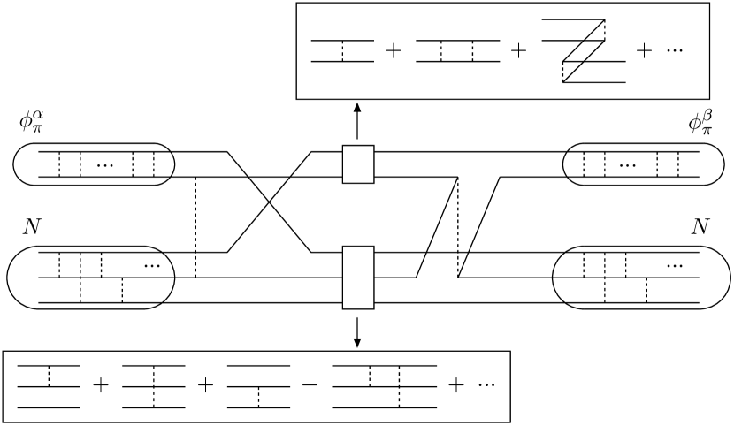
Figure 1: Example of a diagram with intermediate hadrons

In the remainder of his paper we will derive the $\pi-$Baryon ($\pi-B$) scattering lengths, $a_{\pi-B}$.

3 The Resonating Group Method evaluation of $a_{\pi-B}$

Figure 2: Energy, kinetic and potential overlaps contributing to meson-hadron scattering. The dot corresponds to the insertion of a kinetic operator.

To compute the $T_{\pi-B}$ transition matrix we follow the RGM to obtain the effective $\pi-B$ potential $\mathcal{O}^{\mbox{\tiny RGM}}_{\pi-B}$. To see how to derive the RGM formalism for eNJL Hamiltonians see ref. [14, 17, 18, 19, 20, 21], where it was shown that the RGM equations for hadronic scattering, being dynamical equations for coupled channels of boundstates and resonances scattering, are simply obtained by replacing in the S matrix Dyson equations the correspondent solutions of the Bethe-Salpeter equations for each of the intervening hadrons. We get

$$\mathcal{O}^{\mbox{\tiny RGM}}_{\pi-B}=\langle 3E-6T_{1}-6T_{2}-3T_{5}-3V_{23}+3V_{14}+6V_{25}+3A_{15}\rangle\ ,$$ (4)

where the factors 3 and 6 are there to account for all the possible permutations in the exchange of quarks and the minus signs are produced by the Pauli principle. The existence of negative energy spin amplitudes for the mesons complicates considerably the RGM calculations. In order to take into account this degree of freedom we will proceed in two steps. First we will only consider those diagrams containing positive energy amplitudes and later we extend this set of diagrams to those containing the negative energy amplitudes. For the moment let us consider only the positive energy amplitudes.

The different terms of Eq. (4) are represented by the diagrams in Fig. 2. For instance diagrams $\langle E\rangle$ and $\langle V_{14}\rangle$ correspond to the integrals

$$\langle E\rangle = \sum_{s_{i}}\int{\frac{d^{3}p}{(2\pi)^{3}}}{\frac{d^{3}k}{(2\pi)^{3}}}\Psi_{s_{1},s_{2},s_{3}}^{\dagger}(\mbox{\boldmath$p$},\mbox{\boldmath$k$})\ \Psi_{s_{4},s_{2},s_{3}}(\mbox{\boldmath$p$},\mbox{\boldmath$k$})\ \phi_{s_{1},s_{5}}^{\dagger}(\mbox{\boldmath$p$})\ \phi_{s_{4},s_{5}}(\mbox{\boldmath$p$})\ ,$$ (5)

$$\langle V_{14}\rangle = \sum_{s_{i}}\int{\frac{d^{3}p}{(2\pi)^{3}}}{\frac{d^{3}p^{\prime}}{(2\pi)^{3}}}{\frac{d^{3}k}{(2\pi)^{3}}}\Psi_{s_{1},s_{2},s_{3}}^{\dagger}(\mbox{\boldmath$p$},\mbox{\boldmath$k$})\ \Psi_{s_{7},s_{2},s_{3}}(\mbox{\boldmath$p$},\mbox{\boldmath$k$})$$ (6)

$$\hskip 28.45274pt\Gamma^{qq}_{s_{1},s_{6}}(\mbox{\boldmath$p$},\mbox{\boldmath$p^{\prime}$})\ V(\mbox{\boldmath$p$}-\mbox{\boldmath$p^{\prime}$})\ \Gamma^{qq}_{s_{4},s_{7}}(\mbox{\boldmath$p^{\prime}$},\mbox{\boldmath$p$})\ \phi^{\dagger}_{s_{4},s_{5}}(\mbox{\boldmath$p^{\prime}$})\ \phi_{s_{6},s_{5}}(\mbox{\boldmath$p^{\prime}$})\ ,$$

where $V(\mbox{\boldmath$p$}-\mbox{\boldmath$p^{\prime}$})$ represents the Fourier transform of a generic quark kernel $K(x-y)$ which we do not need to know. In Eq. (6) $\phi$ and $\Psi$ are the Salpeter amplitudes for pions and baryons respectively.

Fig. 2 includes all topologically possible diagrams, except for diagrams which interaction can be included from the onset in the energy of the external bound states. All diagrams, except for $\langle A_{15}\rangle$, include a quark exchange because a simple kernel insertion (which goes with ${\vec{\lambda}\over 2}\cdot{\vec{\lambda}\over 2}$ in color space) has zero matrix element between color singlets.

The diagrams $\langle V_{14}\rangle$ and $\langle V_{25}\rangle$ are the usual RGM diagrams yielding for most reactions a repulsive force. This is the case of Nucleon-Nucleon elastic scattering where they are shown to provide a substantial repulsion [22, 26]. The same happens with exotic meson-meson reactions. Retrospectively we can say that the success of the present calculation constitutes an extension of these results.

The diagram $\langle A_{15}\rangle$ contains quark-antiquark annihilation amplitudes and for most cases it provides for attraction [27].

Then $a_{\pi-B}$ is given by

$$a_{\pi-B}=-\mu_{red}\mathcal{O}^{\mbox{\tiny RGM}}_{\pi-B}/(2\pi+2\mu_{red}\mathcal{O}^{\mbox{\tiny RGM}}_{\pi-B}N^{2/3}).$$ (7)

In Eq. (7) $\mu_{red}$ is the reduced mass of the system $\pi-B$,

$$\mu_{red}=M_{\pi}-M_{\pi}^{2}/M_{B}+\cdots\ ,$$ (8)

and the simple Born approximation already provides the leading order in $M_{\pi}$

$$a_{\pi-B}=-M_{\pi}\mathcal{O}^{\mbox{\tiny RGM}}_{\pi-B}/(2\pi)\ .$$ (9)

In order to calculate $\mathcal{O}^{\mbox{\tiny RGM}}_{\pi-B}$ we need first to know the Salpeter solutions for the asymptotic pions and baryons which will then act as wave-functions for the ordinary RGM equations. As we have already stated this recipe is equivalent to solve the complete Dyson series for $\pi-B$ scattering for contact diagrams. For a detailed proof of this equivalence see ref. [14, 17, 18, 19, 20, 21].

4 Salpeter equations for mesons and baryons

In this section we give the Salpeter amplitudes for mesons and $B$s. Since we are considering s-wave hadrons the angular momentum is trivial, and the spin is expected to dominate dynamics. The independent spin degrees of freedom correspond to a spin singlet and a spin triplet. For instance, in the $\Delta$ the diquarks are in a spin triplet state whereas in the $N$ they have a mixed spin structure $(F_{\mbox{\tiny{spin}}}F_{\mbox{\tiny{flavor}}}+D_{\mbox{\tiny{spin}}}D_{\mbox{\tiny{flavor}}})/\sqrt{2}$, where the $F$ component is a singlet and the $D$ component a triplet. In the meson sector the spin structure is clearer. The $\pi$ meson is a spin singlet and the $\rho$ meson is a spin triplet. Besides spin structure we have another degree of freedom known as the energy-spin which takes into account the positive ad negative energy Salpeter amplitudes. These negative energy amplitudes play a major role in the Goldstone nature of the pion, being much less relevant for the $\rho$ case. In the present work these mesonic negative energy amplitudes will be fully taken into account. There are no negative energy amplitudes for the $B$s [28].

Figure 3: Salpeter coupled equations for a quark and an antiquark in a meson. In most mesons the negative energy component $\phi^{-}$ is negligible which simplifies the equation to a single Schrödinger equation

The bound state equations for hadrons are essentially quark-antiquark Salpeter or RPA equation in the case of mesons, see Fig. 3, and Schrödinger or TDA equation for three quarks case of baryons, see Fig. 4. In Fig. 3 the mesonic Salpeter equation consists in fact of two coupled equations, coupling positive to negative energy amplitudes. As an example, we can use the vertices definitions of Table 1 to write one of these equations (the topmost) as

$$\begin{split}H\phi^{+}_{s_{1},s_{2}}(p)&=[T_{p}+T_{-p}]\phi^{+}_{s_{1},s_{2}}(p)+\\ &\hskip 14.22636pt+\sum_{s_{3},s_{4}}\int{d^{3}p^{\prime}\over(2\pi)^{3}}\Gamma^{qq}_{s_{1},s_{3}}(\mbox{\boldmath$p$},\mbox{\boldmath$p$}^{\prime})V(\mbox{\boldmath$p$}-\mbox{\boldmath$p$}^{\prime})\Gamma^{\bar{q}\bar{q}}_{s_{2},s_{4}}(\mbox{\boldmath$p$}^{\prime},\mbox{\boldmath$p$})\phi^{+}_{s_{3},s_{4}}(p^{\prime})+\\ &\hskip 14.22636pt+\sum_{s_{3},s_{4}}\int{d^{3}p^{\prime}\over(2\pi)^{3}}\Gamma^{q\bar{q}}_{s_{1},s_{3}}(\mbox{\boldmath$p$},\mbox{\boldmath$p$}^{\prime})V(\mbox{\boldmath$p$}-\mbox{\boldmath$p$}^{\prime})\Gamma^{\bar{q}q}_{s_{2},s_{4}}(\mbox{\boldmath$p$}^{\prime},\mbox{\boldmath$p$})\phi^{-}_{s_{3},s_{4}}(p^{\prime})\\ &=E\phi^{+}_{s_{1},s_{2}}(p)\ .\end{split}$$ (10)

In particular Eq. (10) reduces to the Schrödinger equation for mesons when the coupling to the negative energy $\phi^{-}$ wave-function is negligible.

Figure 4: Schrödinger equation for 3 quarks in a baryon

The next step consists in working out the spin$\times$flavour$\times$colour traces. These traces are worked out in appendix A. Doing this will lead us, in the case of mesons, to the following two coupled channel equations,

$$H_{m}(\mbox{\boldmath$p$})\;\raisebox{-6.0pt}{$\left[\begin{array}[]{c}|\phi_{m}^{+}\rangle\\ |\phi_{m}^{-}\rangle\end{array}\right]$}\;=\int\frac{d^{3}q}{(2\pi)^{3}}\mathcal{H}(\mbox{\boldmath$p$},\mbox{\boldmath$q$})\raisebox{-6.0pt}{$\left[\begin{array}[]{c}|\phi_{m}^{+}\rangle\\ |\phi_{m}^{-}\rangle\end{array}\right]$}=M_{m}\sigma^{3}\raisebox{-6.0pt}{$\left[\begin{array}[]{c}|\phi_{m}^{+}\rangle\\ |\phi_{m}^{-}\rangle\end{array}\right]$}\ ,$$ (11)

with

$$\mathcal{H}(\mbox{\boldmath$p$},\mbox{\boldmath$q$})=\raisebox{-6.0pt}{$\left[\begin{array}[]{cc}2T_{p}\,\delta(\mbox{\boldmath$p$}-\mbox{\boldmath$q$})+V_{m}^{++}(\mbox{\boldmath$p$},\mbox{\boldmath$q$})&V_{m}^{+-}(\mbox{\boldmath$p$},\mbox{\boldmath$q$})\\ V_{m}^{-+}(\mbox{\boldmath$p$},\mbox{\boldmath$q$})&2T_{p}\,\delta(\mbox{\boldmath$p$}-\mbox{\boldmath$q$})+V_{m}^{--}(\mbox{\boldmath$p$},\mbox{\boldmath$q$})\end{array}\right]$}\ ,$$ (12)

where $V_{m}^{++}$, $V_{m}^{+-}$, $V_{m}^{-+}$ and $V_{m}^{--}$ contain the aforementioned spin traces.

4.1 The pion case

First we work out the spin traces for the pion case. We have,

$$\begin{split}V_{\pi}^{++}(\mbox{\boldmath$p$},\mbox{\boldmath$p$}^{\prime})&=\frac{4}{3}\ Tr\{\Sigma^{\pi}\cdot\Gamma^{\bar{q}\bar{q}}_{p,p^{\prime}}\cdot{\Sigma^{\pi}}^{\dagger}\cdot\Gamma^{qq}_{p^{\prime},p}\}V(\mbox{\boldmath$p$}-\mbox{\boldmath$p$}^{\prime})\\ &=-\frac{2}{3}\ Tr\{\Gamma^{qq}_{p,p^{\prime}}\Gamma^{qq}_{p^{\prime},p}\}V(\mbox{\boldmath$p$}-\mbox{\boldmath$p$}^{\prime})\ ,\\ V_{\pi}^{+-}(\mbox{\boldmath$p$},\mbox{\boldmath$p$}^{\prime})&=\frac{4}{3}\ Tr\{\Sigma^{\pi}\cdot\Gamma^{\bar{q}q}_{p,p^{\prime}}\cdot\Sigma^{\pi}\cdot\Gamma^{\bar{q}q}_{p^{\prime},p}\}V(\mbox{\boldmath$p$}-\mbox{\boldmath$p$}^{\prime})\\ &=-\frac{2}{3}\ Tr\{\Gamma^{q\bar{q}}_{p,p^{\prime}}\Gamma^{\bar{q}q}_{p^{\prime},p}\}V(\mbox{\boldmath$p$}-\mbox{\boldmath$p$}^{\prime})\ .\end{split}$$ (13)

where $\Sigma^{\pi}$ stands for the pion spin wave function defined in Appendix A along with spin wave functions for other relevant hadrons. Notice that $V_{\pi}^{+-}$ acts as a potential coupling the negative energy wave-function $\phi^{-}$ with the positive energy wave-function $\phi^{+}$. $V_{\pi}^{++}$ stands as the usual potential binding the quark and the antiquark in the positive energy wave-function $\phi^{+}$. The color factor 4/3 is included in the $V$’s definition for simplicity. The relations

$$\Gamma^{qq}=(i\sigma_{2})\Gamma^{\bar{q}\bar{q}}(i\sigma_{2})\ ,\hskip 56.9055pt\Gamma^{q\bar{q}}=-(i\sigma_{2})\Gamma^{\bar{q}q}(i\sigma_{2})\ ,$$ (14)

were used. They hold for both the Dirac vertices $\gamma^{0}$ and $\vec{\gamma}$.

The pion occupies a singular position, insofar it is the only bound state where $\phi^{-}_{\pi}$ is not negligible. In particular $|\phi^{-}_{\pi}|$ is just slightly smaller than $|\phi^{+}_{\pi}|$ because the $\pi$ is nearly a Goldstone boson. The Salpeter pion wave functions are

$$\phi^{\pm}(\mbox{\boldmath$k$})=\frac{S(\mbox{\boldmath$k$})}{a}\pm a\,\xi(\mbox{\boldmath$k$})\mbox{\hskip 28.45274ptwith\hskip 14.22636pt}a=\sqrt{\frac{2M_{\pi}}{3}}f_{\pi}\ ,$$ (15)

where $f_{\pi}$ is the well known pion decay constant, $S(k)$ determines the extent of dynamical chiral symmetry breaking and $\xi(k)$ is related to normalization of the wave function. The Salpeter wave functions are normalized as follows,

$$\begin{split}&\left[\begin{array}[]{cc}\langle\phi^{+}|&\langle\phi^{-}|\end{array}\right]\sigma^{3}\raisebox{-6.0pt}{$\left[\begin{array}[]{c}|\phi^{+}\rangle\\ |\phi^{-}\rangle\end{array}\right]$}=\int\frac{d^{3}k}{(2\pi)^{3}}(\phi^{+}(\mbox{\boldmath$k$})^{2}-\phi^{-}(\mbox{\boldmath$k$})^{2})=\\ &=4\int\frac{d^{3}k}{(2\pi)^{3}}S(\mbox{\boldmath$k$})\xi(\mbox{\boldmath$k$})=\frac{2}{a}\int\frac{d^{3}k}{(2\pi)^{3}}S(\mbox{\boldmath$k$})(\phi^{+}(\mbox{\boldmath$k$})-\phi^{+}(\mbox{\boldmath$k$}))=1\ .\end{split}$$ (16)

4.2 The rho case

For the $\rho$ we can follow exactly the same steps as in the pion case to get

$$V_{\rho}^{++}(\mbox{\boldmath$p$},\mbox{\boldmath$p$}^{\prime})=-\frac{2}{9}Tr\{\sigma^{k}\Gamma^{qq}_{p,p^{\prime}}\sigma^{k}\Gamma^{qq}_{p^{\prime},p}\}\delta_{ss^{\prime}}V(\mbox{\boldmath$p$}-\mbox{\boldmath$p$}^{\prime})\ .$$ (17)

To obtain Eq. (17) the following identity

$$\int\frac{d^{3}p}{(2\pi)^{3}}\frac{d^{3}p^{\prime}}{(2\pi)^{3}}Tr\{\sigma^{i}\Gamma^{qq}_{p,p^{\prime}}\sigma^{j}\Gamma^{qq}_{p^{\prime},p}\}=\int\frac{d^{3}p}{(2\pi)^{3}}\frac{d^{3}p^{\prime}}{(2\pi)^{3}}\frac{1}{3}Tr\{\sigma^{k}\Gamma^{qq}_{p,p^{\prime}}\sigma^{k}\Gamma^{qq}_{p^{\prime},p}\}\delta^{ij}\ ,$$ (18)

must be used.

The potential $V_{\rho}^{+-}(\mbox{\boldmath$p$},\mbox{\boldmath$p$}^{\prime})$ can also be computed and it turns out that it is exactly equal to $-1/3$ of $V_{\pi}^{+-}(\mbox{\boldmath$p$},\mbox{\boldmath$p$}^{\prime})$. It provides a negligible coupling of $\phi_{\rho}^{-}$ to $\phi_{\rho}^{+}$ and this is the technical reason why the $\rho$ is essentially a Schrödinger bound state.

4.3 The baryon case

In the case of the baryons we have no negative energy amplitude (there is no way with a two body kernel of simultaneously reversing three quark lines) and we need only to consider the $V_{B}^{++}$. Following the same steps used in deriving Eqs. (13) and (17) we get,

$$\begin{split}V_{N^{F}}^{++}(\mbox{\boldmath$p$},\mbox{\boldmath$p$}^{\prime})&=3\frac{2}{3}\ Tr\{\Sigma^{N^{F}}_{s}\cdot\Gamma^{qq}_{p-k,p^{\prime}-k}\cdot{\Sigma^{N^{F}}_{s^{\prime}}}^{\dagger}\cdot\Gamma^{qq}_{p,p^{\prime}}\}\ V(\mbox{\boldmath$p$}-\mbox{\boldmath$p$}^{\prime})\\ &=-2\frac{1}{2}\ Tr\{\Gamma^{qq}_{p^{\prime}-k,p-k}\Gamma^{qq}_{p,p^{\prime}}\}\ \delta_{ss^{\prime}}V(\mbox{\boldmath$p$}-\mbox{\boldmath$p$}^{\prime})\\ &=-Tr\{\Gamma^{qq}_{p^{\prime}-k,p-k}\Gamma^{qq}_{p,p^{\prime}}\}\ \delta_{ss^{\prime}}V(\mbox{\boldmath$p$}-\mbox{\boldmath$p$}^{\prime}),\end{split}$$ (19)

$$\begin{split}V_{N^{D}}^{++}(\mbox{\boldmath$p$},\mbox{\boldmath$p$}^{\prime})&=3\frac{2}{3}\ Tr\{\Sigma^{N^{D}}_{s}\cdot\Gamma^{qq}_{p-k,p^{\prime}-k}\cdot{\Sigma^{N^{D}}_{s^{\prime}}}^{\dagger}\cdot\Gamma^{qq}_{p,p^{\prime}}\}\ V(\mbox{\boldmath$p$}-\mbox{\boldmath$p$}^{\prime})\\ &=-2\frac{1}{6}\ Tr\{\sigma^{i}\Gamma^{qq}_{p^{\prime}-k,p-k}\sigma^{j}\Gamma^{qq}_{p,p^{\prime}}\}\ \sigma^{i}_{sc}\sigma^{j}_{cs^{\prime}}V(\mbox{\boldmath$p$}-\mbox{\boldmath$p$}^{\prime})\\ &=-\frac{1}{3}\ Tr\{\sigma^{k}\Gamma^{qq}_{p^{\prime}-k,p-k}\sigma^{k}\Gamma^{qq}_{p,p^{\prime}}\}\ \delta_{ss^{\prime}}V(\mbox{\boldmath$p$}-\mbox{\boldmath$p$}^{\prime}),\end{split}$$ (20)

$$\begin{split}V_{\Delta}^{++}(\mbox{\boldmath$p$},\mbox{\boldmath$p$}^{\prime})&=3\frac{2}{3}\ Tr\{\Sigma^{\Delta}_{s}\cdot\Gamma^{qq}_{p-k,p^{\prime}-k}\cdot{\Sigma^{\Delta}_{s^{\prime}}}^{\dagger}\cdot\Gamma^{qq}_{p,p^{\prime}}\}\ V(\mbox{\boldmath$p$}-\mbox{\boldmath$p$}^{\prime})\\ &=-3\frac{1}{3}\ Tr\{\sigma^{i}\Gamma^{qq}_{p^{\prime}-k,p-k}\sigma^{j}\Gamma^{qq}_{p,p^{\prime}}\}\ {w^{i}_{sc}}^{\dagger}w^{j}_{cs^{\prime}}V(\mbox{\boldmath$p$}-\mbox{\boldmath$p$}^{\prime})\\ &=-\frac{1}{3}\ Tr\{\sigma^{k}\Gamma^{qq}_{p^{\prime}-k,p-k}\sigma^{k}\Gamma^{qq}_{p,p^{\prime}}\}\delta_{ss^{\prime}}V(\mbox{\boldmath$p$}-\mbox{\boldmath$p$}^{\prime}).\end{split}$$ (21)

Along with the color factors we include the factor three that accounts for the number of diagrams. We checked numerically, for various microscopic kernels (like for example the $r^{2}$ harmonic kernel) that, under integration in $k$, $V_{N^{F}}^{++}$, $V_{N^{D}}^{++}$ and $V_{\Delta}^{++}$ are, to a good approximation, given by,

$$\begin{split}V_{N^{F}}^{++}(\mbox{\boldmath$p$},\mbox{\boldmath$p$}^{\prime})&\simeq\frac{3}{2}V_{\pi}^{++}(\mbox{\boldmath$p$},\mbox{\boldmath$p$}^{\prime})\delta_{ss^{\prime}},\\ V_{N^{D}}^{++}(\mbox{\boldmath$p$},\mbox{\boldmath$p$}^{\prime})&\simeq\frac{3}{2}V_{\rho}^{++}(\mbox{\boldmath$p$},\mbox{\boldmath$p$}^{\prime})\delta_{ss^{\prime}},\\ V_{\Delta}^{++}(\mbox{\boldmath$p$},\mbox{\boldmath$p$}^{\prime})&\simeq\frac{3}{2}V_{\rho}^{++}(\mbox{\boldmath$p$},\mbox{\boldmath$p$}^{\prime})\delta_{ss^{\prime}},\end{split}$$ (22)

For the various quark kernels, the errors for the $N$ and $\Delta$ masses when using Eqs. (22) instead of Eqs. (19), (20) and (21), were always below $7\%$.

Having the spin$\times$flavor nucleon structure in mind – see Appendix A – we get,

$$V^{++}_{N} = \frac{3}{4}(V^{++}_{\pi}+V^{++}_{\rho})\delta_{ss^{\prime}}\ ,$$

$$V^{++}_{\Delta} = \frac{3}{2}V^{++}_{\rho}\delta_{ss^{\prime}}\ .$$ (23)

In this case the baryon Salpeter amplitude will depend only on the diquark inner momentum and the baryon Salpeter amplitude is given by,

$$\Psi(\mbox{\boldmath$p$})\simeq S(p)/\mathcal{N}$$ (24)

where $\mathcal{N}$ is the baryon wave function normalization which is essentially the same for both $N$ and $\Delta$.

4.4 Summary

The results of the previous subsections can be summarized as follows,

$$\begin{split}&H_{\pi}\;\raisebox{-6.0pt}{$\left[\begin{array}[]{c}|\phi_{\pi}^{+}\rangle\\ |\phi_{\pi}^{-}\rangle\end{array}\right]$}\;=\;\int\frac{d^{3}q}{(2\pi)^{3}}\mathcal{H}_{\pi}(\mbox{\boldmath$p$},\mbox{\boldmath$q$})\raisebox{-6.0pt}{$\left[\begin{array}[]{c}|\phi_{\pi}^{+}\rangle\\ |\phi_{\pi}^{-}\rangle\end{array}\right]$}=M_{\pi}\sigma^{3}\raisebox{-6.0pt}{$\left[\begin{array}[]{c}|\phi_{\pi}^{+}\rangle\\ |\phi_{\pi}^{-}\rangle\end{array}\right]$};\\ &H_{\rho}|\phi_{\rho}\rangle=\int\frac{d^{3}q}{(2\pi)^{3}}\mathcal{H}_{\rho}(\mbox{\boldmath$p$},\mbox{\boldmath$q$})|\phi_{\rho}\rangle=M_{\rho}|\phi_{\rho}\rangle;\\ &\mathcal{H}_{\rho}(\mbox{\boldmath$p$},\mbox{\boldmath$q$})=\left[2T_{p}\,\delta(\mbox{\boldmath$p$}-\mbox{\boldmath$q$})+V^{++}_{\rho}(\mbox{\boldmath$p$},\mbox{\boldmath$q$})\right];\\ &H_{N}|\Psi_{N}\rangle=\int\frac{d^{3}q}{(2\pi)^{3}}\mathcal{H}_{N}(\mbox{\boldmath$p$},\mbox{\boldmath$q$})|\Psi_{N}\rangle=M_{N}|\Psi_{N}\rangle;\\ &\mathcal{H}_{N}(\mbox{\boldmath$p$},\mbox{\boldmath$q$})=\frac{3}{2}\left[2T_{p}\,\delta(\mbox{\boldmath$p$}-\mbox{\boldmath$q$})+\frac{V^{++}_{\pi}(\mbox{\boldmath$p$},\mbox{\boldmath$q$})+V^{++}_{\rho}(\mbox{\boldmath$p$},\mbox{\boldmath$q$})}{2}\right];\\ &H_{\Delta}|\Psi_{\Delta}\rangle=\int\frac{d^{3}q}{(2\pi)^{3}}\mathcal{H}_{\Delta}(\mbox{\boldmath$p$},\mbox{\boldmath$q$})|\Psi_{\Delta}\rangle=M_{\Delta}|\Psi_{\Delta}\rangle;\\ &\mathcal{H}_{\Delta}(\mbox{\boldmath$p$},\mbox{\boldmath$q$})=\frac{3}{2}\left[2T_{p}\,\delta(\mbox{\boldmath$p$}-\mbox{\boldmath$q$})+V^{++}_{\rho}(\mbox{\boldmath$p$},\mbox{\boldmath$q$})\right]\ .\end{split}$$ (25)

Eq. (25) predicts that $M_{\Delta}=(3/2)M_{\rho}$. This is a natural relation in the quark model and it is experimentally correct within $7\%$ discrepancy. This suggests that neglecting both the negative energy wave-function $\phi^{-}_{\rho}$ and the diquark recoil in the baryons are not unreasonable approximations for low energy scattering (scattering lengths).

5 Assembling the $\pi-B$ RGM overlaps $\mathcal{O}^{\mbox{\tiny RGM}}_{\pi-B}$

Before computing the flavor contribution to the RGM overlaps of Fig. 2, we have to extend the class of diagrams in Fig. 2 including the diagrams that couple to the negative energy wave function $\phi^{-}_{\pi}$ of the external pions. The negative energy wave function is defined in Fig. 3 and in Eqs. (10) and (15).

Figure 5: Including the negative energy wave functions $\phi^{-}_{\pi}$ in the RGM overlaps.