FZJ-IKP(TH)-2001-09 Resonance saturation for four–nucleon operators

Abstract

In the modern description of nuclear forces based on chiral effective field theory, four–nucleon operators with unknown coupling constants appear. These couplings can be fixed by a fit to the low partial waves of neutron–proton scattering. We show that the so determined numerical values can be understood on the basis of phenomenological one–boson–exchange models. We also extract these values from various modern high accuracy nucleon–nucleon potentials and demonstrate their consistency and remarkable agreement with the values in the chiral effective field theory approach. This paves the way for estimating the low–energy constants of operators with more nucleon fields and/or external probes.

PACS: 13.20.Gd, 12.39.Fe, 24.80.+y, 24.85.+p, 24.10.-i, 25.10.+s

I Introduction

Effective chiral Lagrangians can be used to investigate the dynamics of pion, pion–nucleon as well as nucleon–nucleon interactions. In all cases, one has to consider two distinct contributions, namely tree and loop diagrams, which are organized according to the underlying power counting [1, 2]. To a given order, one has to consider all local operators constructed from pions, nucleon fields and external sources in harmony with chiral symmetry, Lorentz invariance and the pertinent discrete symmetries. Beyond (or even at) leading order in the chiral expansion, these operators are accompanied by unknown coupling constants, also called low–energy constants (LECs). In principle, these LECs are calculable from QCD but in practice need to be fixed by a fit to some data or using some model . While in certain cases sufficient data exist allowing one to pin down the LECs, often some reliable estimate for these constants beyond naive dimensional analysis is needed. In the meson sector, the ten LECs of the chiral Lagrangian at next–to–leading order (NLO) have been determined [2] and their values can be understood in terms of masses and coupling constants of the lowest meson resonances of vector, axial–vector, scalar and pseudoscalar character, may be with the exception of the scalar sector with vacuum quantum numbers [5, 6]. This is called resonance saturation, it has been used e.g. to estimate LECs at next–to–next–to–leading order (NNLO) (see e.g. [7]) or for the extended chiral Lagrangian including virtual photons as dynamical degrees of freedom [8] . A similar systematic analysis exists for the finite dimension two couplings of the pion–nucleon effective Lagrangian [11], where it was demonstrated the LECs are saturated in terms of baryon resonance excitation in the s– and u–channel and t–channel meson resonances. Much less is known about dimension three and four couplings, but for certain processes resonance saturation has been shown to work quite well, e.g. in neutral pion photoproduction off protons [12]. A somewhat different scheme (including also meson–resonance loops) was introduced in the study of the baryon octet masses in ref. [13]. The situation is very different concerning few–nucleon systems, where a new type of operators with $2A$ nucleon fields appears (for reactions involving $A\geq 2$ nucleons). Only recently, a complete and precise determination of the four S–wave and five P–wave (LO and NLO) LECs in neutron–proton scattering has become available [14], thus it is timely to ask the question whether the numerical values of these four–nucleon coupling constants can be understood from some kind of resonance saturation. This will be the topic of the present paper. As it will turn out, existing one–boson–exchange (or more phenomenologically constructed) models of the nucleon–nucleon (NN) force allow to explain the LECs in terms of resonance parameters. This paves the way for estimating the low–energy constants of operators with more nucleon fields and/or external probes. Before elaborating on the details, we mention that in studies of pion production in proton–proton collisions or charge symmetry breaking in the NN interaction, ideas of resonance saturation have already been used [17, 18]. Also, Friar [19] has discussed aspects of integrating out heavy meson fields to generate local four–nucleon operators with given LECs but did not attempt a detailed comparison with existing models of the nuclear forces as done here.

The plan of the article is as follows. In Section II we discuss the effective chiral Lagrangian for nucleon–nucleon interactions, in particular the four–nucleon terms and their corresponding couplings constants. We then summarize how these LECs are determined at NLO and give a novel prescription to calcuate the NNLO chiral effective field theory (EFT) potential. In Section III we show how to calculate these LECs from existing boson–exchange or phenomenological potentials and compare the resulting values with the ones obtained in EFT. Section IV is devoted to the study of naturalness of these coupling constants and the implications of Wigner’s spin–isospin symmetry. Our conclusions are summarized in Section V. Some technicalities are relegated to the appendices.

II Chiral Effective Field Theory

A Effective Lagrangian and definition of LECs

To be specific, we briefly discuss the approach to chiral Lagrangians for few–nucleon systems proposed by Weinberg. One starts from an effective chiral Lagrangian of pions and nucleons, including in particular local four–nucleon interactions which describe the short range part of the nuclear force, symbolically

$${\mathcal{L}}_{\rm eff}={\mathcal{L}}_{\pi\pi}+{\mathcal{L}}_{\pi N}+{\mathcal{L}}_{NN}~{},$$ (1)

where each of the terms admits an expansion in small momenta and quark (meson) masses. To a given order, one has to include all terms consistent with chiral symmetry, parity, charge conjugation and so on. The last term in eq.(1) contains the four–, six–, $\ldots$ nucleon terms of interest here. From the effective Lagrangian, one derives the two–nucleon potential. This potential is based on (a modified) Weinberg counting [16], more precisely, one organizes the unitarily transformed infrared non–singular diagrams according to their power (chiral dimension) in small momenta and pion masses (for a detailed discussion, see ref. [16]). To leading order (LO), this potential is the sum of one–pion exchange (OPE) (with point-like coupling) and of two four–nucleon contact interactions without derivatives. The low–energy constants accompanying these terms have to be determined by a fit to some data, like e.g. the two S-wave phase shifts in the low–energy region (for $np$). At next–to–leading order (NLO), one has corrections to the OPE, the leading order two–pion exchange graphs and seven dimension two four–nucleon terms with unknown LECs (for the $np$ system). Finally, at NNLO, one has further renormalizations of the one– and corrections to the two–pion exchange graphs including dimension two pion–nucleon operators. The corresponding LECs can be determined from the chiral perturbation theory (CHPT) analysis of pion–nucleon scattering. The existence of shallow nuclear bound states (and large scattering lengths) forces one to perform an additional nonperturbative resummation. This is done here by obtaining the bound and scattering states from the solution of the Lippmann–Schwinger equation. The potential has to be understood as regularized, and the regularization is dictated by the EFT approach employed here, i.e.

$$V({p},{p}^{\prime}\,)\to f_{R}({p})\,V({p},{p}^{\prime})\,f_{R}({p}^{\prime})~{},$$ (2)

where $f_{R}(p)$ is a regulator function chosen in harmony with the underlying symmetries. Within a certain range of cut–off values, the physics should be independent of its precise form and value [20]. That this is indeed the case has been demonstrated in [14]. The central object of the study presented here are the LECs related to the four–nucleon operators. In a spectroscopic notation these are called $C_{1S0}$, $\tilde{C}_{1S0}$, $C_{3S1}$, $\tilde{C}_{3S1}$, $C_{3D1-3S1}:=C_{\epsilon 1}$, $C_{1P1}$, $C_{3P0}$, $C_{3P1}$, and $C_{3P2}$. In the following, we will collectively denote these as $C_{i}$ and $\tilde{C}_{i}$, respectively. The two LECs $\tilde{C}_{i}$ stem from the two momentum independent four–nucleon operators while the seven $C_{i}$ are related to two–derivative operators as they appear in the effective Lagrangian (we have adopted the notation to the two–nucleon potential given in [21]),

$${\cal L}_{NN} = {\cal L}_{NN}^{(2)}+{\cal L}_{NN}^{(4)}+\ldots,$$ (3)

$${\cal L}_{NN}^{(2)} = -\frac{1}{2}\,C_{S}\,(N^{\dagger}N)\,(N^{\dagger}N)-\frac{1}{2}\,C_{T}\,(N^{\dagger}\sigma_{i}\,N)(N^{\dagger}\sigma_{i}\,N)~{},$$ (4)

$${\cal L}_{NN}^{(4)} = {}-\frac{1}{2}{C}_{1}\left[(N^{\dagger}\partial_{i}N)^{2}+((\partial_{i}N^{\dagger})N)^{2}\right]-\left({C}_{1}-\frac{1}{4}{C}_{2}\right)(N^{\dagger}\partial_{i}N)((\partial_{i}N^{\dagger})N)$$ (12)

$${}+\frac{1}{8}{C}_{2}(N^{\dagger}N)\left[N^{\dagger}\partial_{i}^{2}N+\partial_{i}^{2}N^{\dagger}N\right]$$

$${}-\frac{i}{8}{C}_{5}\epsilon_{ijk}\bigg{\{}\left[(N^{\dagger}\partial_{i}N)((\partial_{j}N^{\dagger})\sigma_{k}N)+((\partial_{i}N^{\dagger})N)(N^{\dagger}\sigma_{j}\partial_{k}N)\right]$$

$${}-(N^{\dagger}N)((\partial_{i}N^{\dagger})\sigma_{j}\partial_{k}N)+(N^{\dagger}\sigma_{i}N)((\partial_{j}N^{\dagger})\partial_{k}N)\bigg{\}}$$

$${}+\frac{1}{4}\left(\left(C_{6}+\frac{1}{4}C_{7}\right)\left(\delta_{ik}\delta_{jl}+\delta_{il}\delta_{kj}\right)+\left(2C_{3}+\frac{1}{2}C_{4}\right)\delta_{ij}\delta_{kl}\right)$$

$${}\quad\quad\quad\times\left[((\partial_{i}\partial_{j}N^{\dagger})\sigma_{k}N)+(N^{\dagger}\sigma_{k}\partial_{i}\partial_{j}N)\right](N^{\dagger}\sigma_{l}N)$$

$${}-\frac{1}{2}\left({C}_{6}\left(\delta_{ik}\delta_{jl}+\delta_{il}\delta_{kj}\right)+C_{4}\delta_{ij}\delta_{kl}\right)(N^{\dagger}\sigma_{k}\partial_{i}N)((\partial_{j}N^{\dagger})\sigma_{l}N)$$

$${}-\frac{1}{8}\left(\frac{1}{2}C_{7}\left(\delta_{ik}\delta_{jl}+\delta_{il}\delta_{kj}\right)-(4C_{3}-3C_{4})\delta_{ij}\delta_{kl}\right)\left[(\partial_{i}N^{\dagger}\sigma_{k}\partial_{j}N)+(\partial_{j}N^{\dagger}\sigma_{k}\partial_{i}N)\right](N^{\dagger}\sigma_{l}N)\,,$$

where $N$ denotes the (non–relativistic) nucleon fields, $N=(p,n)^{T}$, and $\sigma_{l}$ $(l=1,2,3)$ are the Pauli spin matrices, and the summation convention for repeated indices is understood. Since we are not considering external sources here, we only have partial derivatives acting on the nucleon fields. To arrive at this expression for the most general effective Lagrangian with four nucleon field operators, we have made use of partial integration, Fierz transformation and the equation of motion for the nucleons. We also require reparametrization invariance [22] of the Lagrangian, which allows us to further reduce the number of independent terms as compared to [15]. The complete derivation of eq. (3) within the heavy baryon formalism is presented in [21]. Note that the effective Lagrangian (3) corresponds to the rest–frame system of the nucleon with the velocity operator given by $v_{\mu}=(1,0,0,0)$. The resulting NN contact potential reads (in the centre–of–mass (c.m.) system):

$$V_{{\rm cont}} = C_{S}+C_{T}(\vec{\sigma}_{1}\cdot\vec{\sigma}_{2})+C_{1}{\vec{q}\,}^{2}+C_{2}{\vec{k}\,}^{2}+(C_{3}{\vec{q}\,}^{2}+C_{4}{\vec{k}\,}^{2})(\vec{\sigma}_{1}\cdot\vec{\sigma}_{2})+iC_{5}\frac{\vec{\sigma}_{1}+\vec{\sigma}_{2}}{2}\cdot(\vec{q}\times\vec{k})$$ (14)

$${}+C_{6}(\vec{q}\cdot\vec{\sigma}_{1})(\vec{q}\cdot\vec{\sigma}_{2})+C_{7}(\vec{k}\cdot\vec{\sigma}_{1})(\vec{k}\cdot\vec{\sigma}_{2})\,,$$

where $\vec{q}=\vec{p}\,^{\prime}-\vec{p}$ and $\vec{k}=(\vec{p}+\vec{p}\,^{\prime})/2$ are the transfered and the averaged momentum, respectively, and $\vec{p}$ ($\vec{p}\,^{\prime}$) corresponds to the initial (final) momentum of the nucleons in the c.m. system. Closer inspection of eq. (14) might lead to the question why no operators containing the isospin matrices $\tau_{i}$ (where $i=1,2$ labels the nucleons) appear? For example, $\rho$–meson exchange will naturally lead to a contribution $\sim\tau_{1}\cdot\tau_{2}$. In principle, at NLO, one can write down 18 operators in the effective potential and not just 9 as appear here. What seems to be completely missing are the nine operators involving products of isospin matrices. However, we remind the reader that only 9 of these 18 operators are independent. The terms in the Lagrangian related to the other 9 can be eliminated using Fierz transformations [1, 16]. Equivalently, one can perform an antisymmetrization of the two–nucleon potential to eliminate redundant terms as used in [23, 14, 21]. Clearly, the set of operators we choose to work with is one but not the unique possibility.

As stated before, there are two/seven LECs related to operators with zero/two derivatives. These constants can be most easily determined by a fit to the S– and P–wave phase shifts and the ${}^{3}S_{1}-^{3}D_{1}$ mixing parameter at low energies, which leads naturally to certain linear combinations, i.e. the already enumerated spectroscopic LECs. The precise relation of the LECs appearing in the effective Lagrangian to the spectroscopic ones is taken from ref.[14] (correcting some typographical errors in that reference),

$$\tilde{C}_{1S0} = {4\pi}\,(C_{S}-3C_{T})~{},$$ (15)

$$C_{1S0} = \pi\,(4C_{1}+C_{2}-12C_{3}-3C_{4}-4C_{6}-C_{7})~{},$$ (16)

$$\tilde{C}_{3S1} = {4\pi}\,(C_{S}+C_{T})~{},$$ (17)

$$C_{3S1} = \frac{\pi}{3}\,(12C_{1}+3C_{2}+12C_{3}+3C_{4}+4C_{6}+C_{7})~{},$$ (18)

$$C_{1P1} = \frac{2\pi}{3}\,(-4C_{1}+C_{2}+12C_{3}-3C_{4}+4C_{6}-C_{7})~{},$$ (19)

$$C_{3P1} = \frac{2\pi}{3}\,(-4C_{1}+C_{2}-4C_{3}+C_{4}+2C_{5}-8C_{6}+2C_{7})~{}$$ (20)

$$C_{3P_{2}} = \frac{2\pi}{3}\,(-4C_{1}+C_{2}-4C_{3}+C_{4}-2C_{5})~{},$$ (21)

$$C_{3P0} = \frac{2\pi}{3}\,(-4C_{1}+C_{2}-4C_{3}+C_{4}+4C_{5}+12C_{6}-3C_{7})~{},$$ (22)

$$C_{3D1-3S1} = C_{\epsilon 1}=\frac{2\sqrt{2}\pi}{3}\,(4C_{6}+C_{7})~{}.$$ (23)

B LECs at next–to–leading order

Let us now discuss the determination of NLO LECs of the chiral EFT potential. In contrast to what was done in [14], we also include the leading charge dependence effect, which is the charged to neutral pion mass difference, $\Delta M_{\pi}=M_{\pi^{\pm}}-M_{\pi^{0}}$, in the OPE potential (for a systematic study of such effects, see [24].) Fitting the low neutron–proton (np) partial waves (S,P and the triplet S-D mixing) for center–of–mass energies below 50-100 MeV, one obtains the numerical values of the LECs for the given regulator and cut–off value. We work here with an exponential regulator,

$$f_{R}(p)=\exp\left(-p^{4}/\Lambda^{4}\right)~{},$$ (24)

where the momentum cut–off $\Lambda$ is varied between 500 and 600 MeV (a more detailed discussion of various regulator functions is given in [14]). Therefore, we obtain a range of values for each LEC in the given partial waves. For a direct comparison with one–boson–exchange models, we need to further add the TPE contribution which stems from the box, triangle and football diagrams. This is done by expanding the contributions of these graphs in terms of local operators with increasing powers of derivatives and projecting onto the appropriate partial waves (this method is described in more detail below). The so obtained numerical contributions in each partial wave are listed in table I in the column TPE(NLO) (for explicit analytical expressions, see appendix A). Obviously, these numbers are cut–off independent. In contrast, the OPE is retained because all potentials we will compare to include it as well. We note that some of these potentials contain a pion–nucleon form factor, but since it only depends on the momentum transfer squared and appears quadratically, it does not influence any four–nucleon operator with zero or two derivatives. With this in mind, we present in table I the resulting values of the LECs for the cut–off varying from 500 to 600 MeV. This is the optimal range found in the study of few–nucleon system [14, 25] as well as proton–proton scattering [24] in the framework used here. Note that in principle we could take smaller values for the cut–off. In such a case one would get a slightly less precise description of the data. On the contrary, one could not substantially increase the cut–off values if no unphysical deeply bound states are allowed [14, 26].

C Phase equivalent potentials and LECs at next–to–next–to–leading order

We now turn to the determination of the LECs based on the NNLO potential. Here, we perform a modification as compared to the work presented in ref. [14]. At that order, the pion–nucleon LECs $c_{1,3,4}$ appear, which have been taken from the CHPT analysis of $\pi N$ scattering in the interior of the Mandelstam triangle [27]. As already shown in ref. [11], these values can be understood in terms of baryon and meson resonance excitations, with a particularly strong contribution from the $\Delta(1232)$ resonance. While the natural size for these LECs is 1 GeV^-1, typical values found for $c_{3}$ and $c_{4}$ from $\pi N$ scattering data are $c_{3}=(-4.70\pm 1.16)$ GeV^-1 and $c_{4}=(3.40\pm 0.04)$ GeV^-1, respectively. The resulting TPE with insertion of these operators improves the fit but leads to a very strongly attractive central potential, as witnessed by the appearance of deeply bound states e.g. in the deuteron channel. These states do, however, not influence the low–energy physics in the two–nucleon system. However, the resulting potential is clearly not phase–equivalent to the boson–exchange or phenomenological potentials, in which the parameters are tuned in a way that no such additional bound states appear. There is also a more microscopic argument. In a model allowing for two–boson exchange (like the Bonn model discussed in refs. [28]) such strongly attractive contributions stem from TPE (with intermediate deltas) which are in low angular momentum partial waves almost completely cancelled by two–boson–exchange graphs, in which one of the pions is substituted by a $\rho$–meson, see e.g. [28] and fig. 1. It is even stated in that last reference that “the $2\pi$–contribution appears, in general, too attractive and a consistent and quantitative description of all phase shifts can never be reached”. Further work on a detailed understanding of correlated $\pi\rho$ exchange has been performed by Holinde and collaborators, see [29]. In the EFT approach, the precise order in which the $\pi\rho$ diagrams with intermediate deltas start contributing to four–nucleon operators depends on the representation of the vector fields (and thus need not appear at the same order as the corresponding $2\pi$ graphs). Therefore, we have constructed new chiral potentials at NNLO where in the NNLO TPE graphs we have substituted the $\pi N$ LECs,

$$c_{i}\to\tilde{c}_{i}=c_{i}-c_{i}^{\Delta}~{},\quad i=3,4~{},$$ (25)

using the formalism of ref. [11] to calculate the $c_{i}^{\Delta}$. More precisely, we have allowed for some fine tuning of the $\tilde{c}_{i}$ within the bounds given in that reference. By this method, the equivalent TPE graphs with intermediate deltas are subtracted and the aforementioned cancellations are effectively taken into account. For a typical NNLO fit, we use $c_{1}=-0.81$ GeV^-1, $c_{3}=-1.15$ GeV^-1, and $c_{4}=1.20$ GeV^-1. From that, we obtain the NNLO TPE contribution listed in table I (for explicit analytical expressions, see appendix A). A more detailed description of this procedure and further justification of it will be given in a forthcoming publication [30]. The so determined TPE NNLO contribution and the corresponding LECs are displayed in table I. It is important to note that in the cases where the TPE contribution is large, the NNLO correction is sizeably smaller than the NLO one. The resulting values for the LECs $C_{i}$ and $\tilde{C}_{i}$ at NNLO are consistent with the ones found at NLO. That is an important result.

We are now in the position to confront the LECs determined from chiral effective field theory with the highly successful phenomenological/meson models of the nuclear force. Before doing that, some discussion concerning the NNLO potential constructed in [14] is in order. It is a perfectly viable scenario to use the unsubtracted values for the $c_{i}$ as done there since the resulting deep bound states do not influence the physics in the two–nucleon system. As noted already, a direct comparison of the contact terms in the potential with the ones obtained from the meson–exchange or phenomenological approaches can not be made. While the physics in three– or four–nucleon systems does not depend on the choice of the unsubtracted or subtracted $c_{i}$, the latter choice is closer to standard nuclear physics in which three–body forces lead to small binding energy corrections [30]. In fact, applying directly the potential from ref.[14] to such systems leads to much smaller binding energies from the two–nucleon forces alone. However, such a separation of the total binding energy into NN and 3N contributions is not observable and therefore this scenario is not ruled out. These topics will be discussed in much more detail in [30]. At this stage, both options discussed here are viable. It is fair to say that more detailed calculations in few–nucleon systems have to be performed to ultimately clarify this issue. We proceed using the modified dimension two pion–nucleon couplings, cf. eq.(25).

III LECs from boson–exchange and phenomenological NN potentials

We consider first genuine one–boson–exchange models of the NN force, in which the long range part of the interaction is given by OPE (including in general a pion–nucleon form factor) whereas shorter distance physics is expressed in terms of a sum over heavier mesons,

$$V_{\rm NN}=V_{\pi}+\sum_{M=\sigma,\rho,\ldots}V_{M}~{},$$ (26)

where some mesons can be linked to real resonances (like e.g. the $\rho$–meson) or are parametrizations of certain physical effects, e.g. the light scalar–isoscalar $\sigma$–meson is needed to supply the intermediate range attraction (but it is not a resonance). The corresponding meson–nucleon vertices are given in terms of one (or two) coupling constant(s) and corresponding form factor(s), characterized by some cut–off $\Lambda_{M}$. These form factors are needed to regularize the potential at small distances (large momenta) but they should not be given a physical interpretation. As depicted in Fig.2, in the limit of large meson masses, keeping the ratio of coupling constant to mass fixed, one can interpret such exchange diagrams as a sum of local operators with increasing number of derivatives (momentum insertions). In a highly symbolic relativistic notation, this reads,

$$(\bar{N}P_{i}N)\left({g^{2}\,\delta^{ij}\over M_{R}^{2}-t}\right)(\bar{N}P_{j}N)=\left({g^{2}\over M_{R}^{2}}\right)(\bar{N}P_{i}N)(\bar{N}P^{i}N)+\left({g^{2}\,t\over M_{R}^{4}}\right)(\bar{N}P_{i}N)(\bar{N}P^{i}N)+\dots~{},$$ (27)

where the $P_{i}$ are projectors on the appropriate quantum numbers for a given meson exchange (including also Dirac matrices if needed) and $M_{R}$ is the mass of corresponding heavy meson. It should be kept in mind here that one usually makes use of the non–relativistic expansion, i.e. the Dirac spinors on the right–hand side of eq. (27) coincide with the Pauli spinors. In case of a momentum–dependent meson–nucleon coupling, like e.g. for a monopole form factor normalized to one at $t=0$,

$$g(t)=g\,{\Lambda_{M}^{2}\over\Lambda_{M}^{2}-t}~{},$$ (28)

then the coefficient of the first $t$–dependent term in Eq.(27) is modified to

$${g^{2}\over M_{R}^{4}}\to{g^{2}\over M_{R}^{2}}\,\left({1\over M_{R}^{2}}+{2\over\Lambda_{M}^{2}}\right)~{},$$ (29)

and accordingly for other types of form factors (dipole, monopole normalized to one at $t=M_{R}^{2}$, etc.). The coupling constants are either determined in the fit to the NN scattering and bound state data or are taken from other sources, the form factor cut–offs always have to be determined from the fit. It is obvious from these considerations that such heavy meson exchanges generate four–nucleon terms with zero, two, four, $\ldots$ derivatives. In appendix B, we collect the explicit formulae for scalar, pseudoscalar and vector meson exchanges, which can be applied to any of the OBE potentials by using the appropriate masses and coupling constants (and should be used instead of the symbolic formulae given before). As a typical example for an OBE potential we consider the Bonn-B variant [31]. Its short range part is build from scalar ($\sigma$, $\delta$), pseudoscalar ($\eta$) and vector meson ($\rho$, $\omega$) exchanges, and the pertinent contributions to the LECs $C_{i},\,\tilde{C}_{i}$ are listed in table II. Another (more recent) OBE potential is the Nijmegen 93 potential (denoted Nijm–93) [32]. The Nijmegen 93 potential is particular since it also includes mesons with strange quarks but total strangeness zero (like the scalar $\epsilon(1300)$ or the $\phi(1020)$) and a low–energy representation of the Pomeron, which usually is needed to describe very high energetic proton–proton scattering. SU(3) flavor symmetry is imposed so that certain couplings are linked. The various contributions to the LECs are displayed in table III. Some of the individual terms are unnaturally large (in particular the ones from the Pomeron), but the total contribution of the scalar sector is quite similar to the ones in the Bonn-B potential, as comparison of tables II,III reveals. The vector meson contributions ($\rho,\omega$) are very similar for both potentials. The resulting LECs for these two OBE potentials are summarized in table IV. While there is some spread in some of the partial waves, the overall agreement with the LECs determined using the chiral EFT potential listed in table I is rather satisfactory but these results are also somewhat surprising, because the phenomenological potential models are not constructed based on any power counting nor chiral symmetry, plus in many cases contain quantum field theoretically ill–defined form factors. Still, it is gratifying to see that the contact part of the NN potential does not depend on how the short distance physics is parametrized. To our knowledge, this is the first time that a direct link between the Weinberg program of systematically deriving nuclear forces from chiral Lagrangians to these phenomenologically successful potentials has been achieved in a truely quantitative manner.

There exists also a different class of potentials, which are constructed to give $\chi^{2}/{\rm datum}\simeq 1$ fits to the NN data base like the high–precision charge–dependent CD–Bonn 2000 [33]. It contains two scalar–isoscalar mesons in each partial wave up to angular momentum $J=5$ with the mass and coupling constant of the second $\sigma$ fine tuned in any partial wave. The other high–precision potentials are the Nijmegen I,II [32] as well as the Argonne V18 (AV–18) [34] potentials. For the former, one–pion exchange is supplemented by heavy boson exchanges with adjustable parameters which are fitted for all (low) partial waves separately. The AV–18 potential starts from a very general operator structure in coordinate space and has fit functions for all these various operators. Note that we have switched off the various electromagnetic corrections implemented in the AV–18 potential code. Such type of potentials can also be expanded in terms of four–nucleon contact operators with increasing dimension. We do not give the details here but only mention that we have done this using numerical methods. The resulting LECs $C_{i}$ and $\tilde{C}_{i}$ are also listed in table IV. In fig.3 we give a graphical representation of the LECs obtained in EFT, cf. table I, compared with the results from the six potential models considered here, see table IV. Note that the various LECs are scaled with different factors, sometimes including an overall minus sign. This is done to achieve a more uniform representation. Note also that the theoretical uncertainties for the LECs determined in EFT are a) small compared to their average values and b) are smaller than the band spanned by the potential models (even if one only includes the high–precision ones).

IV Naturalness of the LECs and Wigner Symmetry

First, we wish to investigate whether the LECs determined in section II are of natural size. In the present context of Weinberg power counting, dimensional scaling arguments allow one to express any term of the effective Lagrangian with nucleon and pion fields as well as derivative and pion mass insertions (for a derivation and further discussion, see e.g. [19]) as

$${\cal L}=c_{lmn}\,\left({N^{\dagger}(\ldots)N\over f_{\pi}^{2}\,\Lambda_{\chi}}\right)^{l}\,\left({\pi\over f_{\pi}}\right)^{m}\,\left({\partial^{\mu},M_{\pi}\over\Lambda_{\chi}}\right)^{n}\,f_{\pi}^{2}\,\Lambda_{\chi}^{2}~{}~{},$$ (30)

where the $c_{lmn}$ are dimensionless numbers and $l,m,n$ are non–negative integers. Here, $2l$ counts the number of nucleon fields, $m$ the number of pions and $n$ the number of derivatives or pion mass insertions. All nucleon isospin operators and so on are non–essential to this formula and indicated by the ellipsis. Note that this naive power counting can not be applied to cases with spurious bound states, as witnessed by the so–called limit cycle behaviour [35, 36, 26]. Here, we only consider potentials with no such spurious bound states, thus the relevant scale for the four–nucleon interactions without derivatives ($l=2,m=n=0$) is the inverse of the pion decay constant, $f_{\pi}=92.4\,$MeV, squared and two derivative terms ($l=2,m=0,n=2$) are suppressed by two inverse powers of the chiral scale $\Lambda_{\chi}\simeq 1$ GeV. For the LECs from the Lagrangian (3) naturalness thus amounts to

$$C_{i}\sim{c_{200}\over f_{\pi}^{2}}~{},\quad(i=S,T)~{},\qquad C_{j}\sim{c_{202}\over f_{\pi}^{2}\,\Lambda_{\chi}^{2}}~{},\quad(i=1,\dots,7)~{},$$ (31)

and the $c_{200}$ and $c_{202}$ should be numbers of order one (if there is not some suppression due to some symmetry, see below). Such arguments can, of course, not say anything about the signs of the LECs. Also, it is important to realize the prefactors which accompany the various terms of the Lagrangian. E.g. there is a relative factor of four in the momentum space representation between terms $\sim{\vec{q}}\,^{2}=(\vec{p}\,^{\prime}-\vec{p}\,)^{2}$ and $\sim\vec{k}\,^{2}=(\vec{p}\,^{\prime}+\vec{p}\,)^{2}/4$. Such factors need to be accounted for. Consequently, we give in table V the corresponding coefficients $c_{200}$ and $c_{202}$ of the LECs as deduced from our NLO and NNLO fits using eqs.(15). Inspection of the table reveals that the numbers fluctuate between 0.3 and 3.5, i.e. the values found for these LECs are indeed natural, with the notable exception of $f_{\pi}^{2}\,C_{T}$, which is much smaller than one (except for the upper limit of NLO cut–offs, which is already close to the edge of having stable fits, see also the discusion in [14]). As just mentioned, symmetry can lead to the suppression (or enhancement) of certain coupling constants. In fact, 65 years ago Wigner [37] proposed that SU(4) spin–isospin transformations are an approximate symmetry of the strong interactions. Such a transformation has the form

$$\delta\,N=i\varepsilon_{\mu\nu}\,\sigma^{\mu}\,\tau^{\nu}\,N~{},\qquad N=\bigg{(}\begin{array}[]{c}p\\ n\end{array}\bigg{)}~{},\qquad\mu,\nu=0,1,2,3~{},$$ (32)

with $\sigma^{\mu}=(1,\vec{\sigma})$, $\tau^{\nu}=(1,\vec{\tau})$, and $\varepsilon_{\mu\nu}$ are infinitesimal group parameters. This symmetry emerges in the large number of color limits of QCD [38] and thus features prominently in the nuclear forces derived from Skyrme type models. It was recently shown [39] that in the limit where the S–wave scattering lengths $a_{1S0}$ and $a_{3S1}$ go to infinity, the leading terms in the EFT for strong NN interactions (with pions treated perturbatively) are invariant under Wigner’s SU(4) spin–isospin transformations. This can be seen most easily from the leading four–nucleon operators as used here, see eq.(3) In this basis, the first term is clearly invariant under Wigner transformations, cf eq.(32), whereas the second term $\sim C_{T}$ obviously breaks the SU(4) symmetry. In the Weinberg approach employed here, the leading order potential consists of these two four–nucleon operators supplemented by the one–pion exchange. Still, the Wigner symmetry is kept intact to a good precision since the resulting fit values for $C_{T}$ are sizeably smaller than the corresponding ones for $C_{S}$, see table V. Stated differently, $C_{T}$ is unnaturally small because of the Wigner symmetry. This can be understood from the fact that at very low energies, where one is essentially sensitive to the (S–wave) scattering lengths, the pion–exchange contribution can be expanded in powers of momenta, leading to terms with at least two derivatives, see appendix B. One thus effectively recovers the situation eluded to in ref.[39]. However, for larger momenta (say of the order of the pion mass), the non–perturbative treatment of the pions as proposed by Weinberg is mandatory.

V Conclusions and Summary

In this manuscript, we have investigated the low–energy constants with zero and two derivatives that appear in the four–nucleon contact interactions of the chiral effective Lagrangian for the nucleon–nucleon forces. Our main findings can be summarized as follows:

• We have determined the LECs for the NLO and NNLO potentials, including the dominant charge–dependence effect from the pion mass difference in the one–pion exchange. To avoid the unphysical bound states at NNLO, we have argued that one has to subtract the delta contribution from the dimension two pion–nucleon LECs. This is in agreement with two–boson–exchange models, where the two–pion–exchange contribution is cancelled largely by $\pi\rho$ graphs.

• We have shown how to deduce similar type of contact operators from boson–exchange models in the limit of large meson masses. This allows to calculate the LECs in terms of meson–nucleon coupling constants, meson masses and (unobservable) cut–off masses. In a similar manner, one can examine the so–called high–precision potential models. We have found that in all cases, the LECs determined from these models are close to the values found in EFT, which can be considered as a new form of resonance saturation.

• We have shown that with the exception of one dimension zero coupling (the LEC $C_{T}$), all LECs are of natural size. The smallness of $C_{T}$ is due to Wigner’s spin–isospin symmetry, as was already pointed out for the case of a theory with pions integrated out or treated perturbatively.

Clearly, these findings have further–reaching consequences. On one side, they might allow to further constrain models of the nucleon–nucleon interaction applicable at energies where the EFT description can not be used. On the other hand, in case of external sources (like e.g. photons) or multi–nucleon operators (as they appear e.g. in the description of the three–body forces), these considerations will allow to at least estimate novel LECs that will appear. In the latter case of three– and more–nucleon systems performing a direct fit with 5 adjustable parameters (if the leading non–vanishing three–nucleon force is included) to 3N observables will be a very expensive task with respect to computer power. Therefore it might be very helpful to have a rough estimation for the values of various couplings appearing in the 3N force.

A Reduction of the two–pion exchange contributions

As stated before, we have to add the contribution of the TPE to the LECs so as to be able to compare with the boson exchange potentials. The explicit expressions for the renormalized TPE potential at NLO can be found in ref.[16]. Expanding those in powers of $\vec{q}$ and $\vec{k}$ allows for a mapping on the spectroscopic LECs (of course, the TPE contains many other contributions, which are, however, of no relevance for this discussion). We get

$$\tilde{C}_{1S0}^{\rm NLO} = -\frac{1}{3}\tilde{C}_{3S1}^{\rm NLO}=\frac{(1+4g_{A}^{2}-8g_{A}^{4})M_{\pi}^{2}}{24\pi f_{\pi}^{4}}~{},$$ (A1)

$$C_{1S0}^{\rm NLO} = \frac{2+17g_{A}^{2}-88g_{A}^{4}}{144\pi f_{\pi}^{4}}~{},$$ (A2)

$$C_{3S1}^{\rm NLO} = -\frac{2+17g_{A}^{2}-40g_{A}^{4}}{48\pi f_{\pi}^{4}}~{},$$ (A3)

$${C}_{\epsilon 1}^{\rm NLO} = -\frac{g_{A}^{4}}{4\sqrt{2}\pi f_{\pi}^{4}}~{},$$ (A4)

$$C_{1P1}^{\rm NLO} = \frac{2+17g_{A}^{2}-16g_{A}^{4}}{72\pi f_{\pi}^{4}}~{},$$ (A5)

$$C_{3P0}^{\rm NLO} = -\frac{2+17g_{A}^{2}+74g_{A}^{4}}{216\pi f_{\pi}^{4}}~{},$$ (A6)

$$C_{3P1}^{\rm NLO} = -\frac{2+17g_{A}^{2}-61g_{A}^{4}}{216\pi f_{\pi}^{4}}~{},$$ (A7)

$$C_{3P2}^{\rm NLO} = -\frac{2+17g_{A}^{2}-7g_{A}^{4}}{216\pi f_{\pi}^{4}}~{}~{}.$$ (A8)

Note that in the chiral limit, the two leading contact interactions do not get renormalized by TPE. Furthermore, these expressions only depend on the lowest order pion–nucleon coupling $\sim g_{A}$ (or, by virtue of the Goldberger–Treiman relation, on $g_{\pi NN}$). Similarly, we can give the additional TPE NNLO contributions to the various LECs (for an explicit expression of the renormalized NNLO TPE potential, see e.g. ref.[14]),

$$\tilde{C}_{1S0}^{\rm NNLO} = \frac{g_{A}^{2}(-16+192m(-2c_{1}+c_{3})+25g_{A}^{2})M_{\pi}^{3}}{256mf_{\pi}^{4}}~{},$$ (A9)

$$\tilde{C}_{3S1}^{\rm NNLO} = \frac{3g_{A}^{2}(16+64m(-2c_{1}+c_{3})-21g_{A}^{2})M_{\pi}^{3}}{256mf_{\pi}^{4}}~{},$$ (A10)

$$C_{1S0}^{\rm NNLO} = \frac{g_{A}^{2}(-368-192m(10c_{1}-11c_{3}+4c_{4})+869g_{A}^{2})M_{\pi}}{3072mf_{\pi}^{4}}~{},$$ (A11)

$$C_{3S1}^{\rm NNLO} = -\frac{g_{A}^{2}(16(-7+4m(10c_{1}-11c_{3}+4c_{4}))+81g_{A}^{2})M_{\pi}}{1024mf_{\pi}^{4}}~{},$$ (A12)

$${C}_{\epsilon 1}^{\rm NNLO} = \frac{g_{A}^{2}(8+32mc_{4}-7g_{A}^{2})M_{\pi}}{64\sqrt{2}mf_{\pi}^{4}}~{},$$ (A13)

$$C_{1P1}^{\rm NNLO} = \frac{g_{A}^{2}(-368+64m(10c_{1}-11c_{3}-12c_{4})+305g_{A}^{2})M_{\pi}}{1536mf_{\pi}^{4}}~{},$$ (A14)

$$C_{3P0}^{\rm NNLO} = \frac{g_{A}^{2}(176+192m(10c_{1}-11c_{3}-8c_{4})+691g_{A}^{2})M_{\pi}}{4608mf_{\pi}^{4}}~{},$$ (A15)

$$C_{3P1}^{\rm NNLO} = \frac{g_{A}^{2}(464+192m(10c_{1}-11c_{3}+2c_{4})-545g_{A}^{2})M_{\pi}}{4608mf_{\pi}^{4}}~{},$$ (A16)

$$C_{3P2}^{\rm NNLO} = -\frac{g_{A}^{2}(112+192m(-10c_{1}+11c_{3}+2c_{4})+281g_{A}^{2})M_{\pi}}{4608mf_{\pi}^{4}}~{},$$ (A17)

with $m$ the nucleon mass. These expressions depend on the dimension two LECs $c_{1,3,4}$ as discussed before. We note that all these contributions vanish in the chiral limit.

B Reduction of one–boson–exchanges

Here, we give the explicit expression for scalar, pseudoscalar and vector meson exchange contributions to four–nucleon operators with zero or two derivatives, as depicted in fig. 2. Note that we will also include $1/m$ as well as $1/m^{2}$ corrections, which are, strictly speaking, of higher orders in the power counting scheme we are working with and not (or partly) present in the NLO and NNLO potentials. There is, however, no contradiction since adding or subtracting those terms from the potential would lead to changes smaller than the level of accuracy of our approach. The contributions for a particular OBE potential can be obtained by using the appropriate masses, coupling constants (and form factors) employed there. To obtain the most general expressions, we include any form factor as

$$F_{M}(\vec{q}\,^{2})=\alpha_{1}+\alpha_{2}\frac{\vec{q}\,^{2}}{\Lambda_{M}^{2}}+{\cal O}(\vec{q}\,^{4})~{},$$ (B1)

where the coefficient $\alpha_{1}=1$ if the form factor is normalized to one at $\vec{q}\,^{2}=0$ or $\alpha_{1}\neq 1$ if the form factor is normalized to one at $\vec{q}\,^{2}=-M^{2}_{M}$ (with $M_{M}$ the mass of the meson under consideration) or it might include the meson–nucleon coupling constant $g_{M}$. We will give generic expression where the corresponding vertices are written as $g_{M}\times F_{M}(\vec{q}\,^{2})$, with $F_{M}$ expanded as just discussed. Note for the exchange of isovector bosons like the $\pi$ or the $\rho$, the given expressions have to be multiplied by a factor $\mbox{\boldmath$\tau$}_{1}\cdot\mbox{\boldmath$\tau$}_{2}$ leading to a factor of (-3) for the $T=0$ potential considered here.

1 Scalar meson exchange

The Lagrangian for coupling of an scalar–isoscalar meson with mass $M_{S}$ and coupling constant $g_{S}$ reads

$${\cal L}_{S}=g_{S}\bar{\psi}\psi\phi~{},$$ (B2)

where $\psi$ denotes the relativistic nucleon field and $\phi$ the scalar meson (for an isovector, one simply replaces $\phi$ by $\mbox{\boldmath$\tau$}\cdot\mbox{\boldmath$\phi$}$, with $\tau^{k}$ ($k=1,2,3$) the usual Pauli isospin matrices). In the non–relativistic expansion, the momentum space expression for the corresponding exchange potential with a form factor (if applicable) characterized by the cut–off $\Lambda_{S}$ reads up to terms of order $1/m^{2}$

$$V_{S}(\vec{q}\,,\vec{k}\,)=-\frac{g_{S}^{2}}{\vec{q}\,^{2}+M_{S}^{2}}\,\left[1-\frac{\vec{k}\,^{2}}{2m^{2}}+\frac{\vec{q}\,^{2}}{8m^{2}}-\frac{i}{2m^{2}}\vec{S}\cdot(\vec{q}\times\vec{k}\,)\right]\,F_{S}^{2}(\vec{q}\,^{2})~{},$$ (B3)

where $\vec{S}=(\vec{\sigma}_{1}+\vec{\sigma}_{2})/2$ is the total spin of the two–nucleon system. The fully relativistic form of this exchange can be found e.g. in ref.[31]. This gives the following contributions to the spectroscopic LECs:

$$\tilde{C}_{1S0}^{S} = \tilde{C}_{3S1}^{S}=-\frac{4\pi g_{S}^{2}\alpha_{1}^{2}}{M_{S}^{2}}~{},$$ (B4)

$$C_{1S0}^{S} = C_{3S1}^{S}=\frac{4\pi g_{S}^{2}\alpha_{1}\,(-2M_{S}^{2}\alpha_{2}+\alpha_{1}\Lambda_{S}^{2})}{M_{S}^{4}\,\Lambda_{S}^{2}}~{},$$ (B5)

$${C}_{\epsilon 1}^{S} = 0~{},$$ (B6)

$$C_{1P1}^{S} = \frac{2\pi g_{S}^{2}\alpha_{1}\,((-4+M_{S}^{2}/m^{2})\alpha_{1}+8M_{S}^{2}\alpha_{2}/\Lambda_{S}^{2})}{3M_{S}^{4}}~{},$$ (B7)

$$C_{3P0}^{S} = \frac{2\pi g_{S}^{2}\alpha_{1}\,(8m^{2}M_{S}^{2}\alpha_{2}-(4m^{2}-3M_{S}^{2})\alpha_{1}\Lambda_{S}^{2})}{3m^{2}M_{S}^{4}\,\Lambda_{S}^{2}}~{},$$ (B8)

$$C_{3P1}^{S} = \frac{4\pi g_{S}^{2}\alpha_{1}\,((-2+M_{S}^{2}/m^{2})\alpha_{1}+4M_{S}^{2}\alpha_{2}/\Lambda_{S}^{2})}{3M_{S}^{4}}~{},$$ (B9)

$$C_{3P2}^{S} = \frac{8\pi g_{S}^{2}\alpha_{1}\,(2M_{S}^{2}\alpha_{2}-\alpha_{1}\Lambda_{S}^{2})}{3M_{S}^{4}\,\Lambda_{S}^{2}}~{}.$$ (B10)

2 Pseudoscalar meson exchange

The Lagrangian for coupling of a scalar–pseudoscalar meson with mass $M_{P}$ and coupling constant $g_{P}$ reads

$${\cal L}_{P}=-g_{P}\bar{\psi}i\gamma^{5}\psi\pi~{},$$ (B11)

where $\pi$ denotes the pseudoscalar meson (for an isovector, one simply replaces $\pi$ by $\mbox{\boldmath$\tau$}\cdot\mbox{\boldmath$\pi$}$). This is the so–called pseudoscalar coupling. Equivalently, one can also use a derivative type (pseudovector) coupling

$${\cal L}_{P}^{\prime}=-\frac{f_{P}}{M_{P}}\bar{\psi}\gamma^{5}\gamma^{\mu}\psi\partial_{\mu}\pi~{}.$$ (B12)

At tree level, these couplings are equivalent provided $g_{P}/m=f_{P}/M_{P}$. Of course, chiral symmetry enforces the derivative coupling for the Goldstone bosons. In the non–relativistic expansion, the momentum space expression for the corresponding exchange potential with a form factor (if applicable) characterized by the cut–off $\Lambda_{P}$ reads up to terms of order $1/m^{2}$

$$V_{P}(\vec{q}\,)=-\frac{g_{P}^{2}}{4m^{2}}\,\frac{(\vec{\sigma}_{1}\cdot\vec{q}\,)(\vec{\sigma}_{2}\cdot\vec{q}\,)}{\vec{q}\,^{2}+M_{P}^{2}}\,F_{P}^{2}(\vec{q}\,^{2})~{}.$$ (B13)

Again, the fully relativistic form of this exchange can be found e.g. in ref.[31]. This gives the following contributions to the spectroscopic LECs:

$$\tilde{C}_{1S0}^{P} = \tilde{C}_{3S1}^{P}=0~{},$$ (B14)

$$C_{1S0}^{P} = -3C_{3S1}^{P}=\Gamma_{P}~{},$$ (B15)

$$-\frac{3}{2\sqrt{2}}C_{\epsilon 1}^{P} = -\frac{3}{2}C_{1P1}^{P}=-\frac{1}{2}C_{3P0}^{P}=\frac{3}{4}C_{3P1}^{P}=\Gamma_{P}~{},$$ (B16)

$$C_{3P2}^{P} = 0~{},$$ (B17)

with

$$\Gamma_{P}=\frac{\pi g_{P}^{2}\alpha_{1}^{2}}{m^{2}M_{P}^{2}}~{}.$$ (B18)

3 Vector meson exchange

The Lagrangian for coupling of a vector meson with mass $M_{V}$ and coupling constants $g_{V}$ (vector coupling) and $f_{V}$ (tensor coupling) reads

$${\cal L}_{V}=-g_{V}\bar{\psi}\gamma^{\mu}\psi\phi_{\mu}-\frac{f_{V}}{4m}\bar{\psi}\sigma^{\mu\nu}\psi(\partial_{\mu}\phi_{\nu}-\partial_{\nu}\phi_{\mu})~{},$$ (B19)

where $\phi_{\mu}$ denotes the isoscalar–vector meson (for an isovector, one simply replaces $\phi_{\mu}$ by $\mbox{\boldmath$\tau$}\cdot\mbox{\boldmath$\phi$}_{\mu}$). In the non–relativistic expansion, the momentum space expression for the corresponding exchange potential with a form factor (if applicable) characterized by the cut–off $\Lambda_{V}$ reads up to terms of order $1/m^{2}$

$$V_{V}(\vec{q}\,,\vec{k}\,) = \frac{1}{\vec{q}\,^{2}+M_{V}^{2}}\,\biggl{\{}g_{V}^{2}\biggl{[}1+\frac{3\vec{k}\,^{2}}{2m^{2}}-\frac{\vec{q}\,^{2}}{8m^{2}}+\frac{3i}{2m^{2}}\vec{S}\cdot(\vec{q}\times\vec{k}\,)-\vec{\sigma}_{1}\cdot\vec{\sigma}_{2}\frac{\vec{q}\,^{2}}{4m^{2}}+\frac{1}{4m^{2}}(\vec{\sigma}_{1}\cdot\vec{q}\,)(\vec{\sigma}_{2}\cdot\vec{q}\,)\biggr{]}$$ (B22)

$$\qquad\qquad+\frac{g_{V}f_{V}}{2m}\biggl{[}-\frac{\vec{q}\,^{2}}{m}+\frac{4i}{m}\vec{S}\cdot(\vec{q}\times\vec{k}\,)-\vec{\sigma}_{1}\cdot\vec{\sigma}_{2}\frac{\vec{q}\,^{2}}{m}+\frac{1}{m}(\vec{\sigma}_{1}\cdot\vec{q}\,)(\vec{\sigma}_{2}\cdot\vec{q}\,)\biggr{]}$$

$$\qquad\qquad+\frac{f_{V}^{2}}{4m^{2}}\left[-\vec{\sigma}_{1}\cdot\vec{\sigma}_{2}\vec{q}\,^{2}+(\vec{\sigma}_{1}\cdot\vec{q}\,)(\vec{\sigma}_{2}\cdot\vec{q}\,)\right]\biggr{\}}~{}F_{V}^{2}(\vec{q}\,^{2})~{},$$

Again, the fully relativistic form of this exchange can be found e.g. in ref.[31]. This gives the following contributions to the spectroscopic LECs:

$$\tilde{C}_{1S0}^{V} = \tilde{C}_{3S1}^{V}=\frac{4\pi g_{V}^{2}\alpha_{1}^{2}}{M_{V}^{2}}~{},$$ (B23)

$$C_{1S0}^{V} = \frac{\pi\alpha_{1}\,(8m^{2}g_{V}^{2}M_{V}^{2}\alpha_{2}-(4m^{2}g_{V}^{2}-(2f_{V}^{2}+2f_{V}g_{V}+3g_{V}^{2})M_{V}^{2})\alpha_{1}\Lambda_{V}^{2})}{m^{2}M_{V}^{4}\,\Lambda_{V}^{2}}~{},$$ (B24)

$$C_{3S1}^{V} = \frac{\pi\alpha_{1}\,(24m^{2}g_{V}^{2}M_{V}^{2}\alpha_{2}-(12m^{2}g_{V}^{2}+(2f_{V}^{2}+10f_{V}g_{V}-g_{V}^{2})M_{V}^{2})\alpha_{1}\Lambda_{V}^{2})}{3m^{2}M_{V}^{4}\,\Lambda_{V}^{2}}~{},$$ (B25)

$${C}_{\epsilon 1}^{V} = \frac{2\sqrt{2}\pi(f_{V}+g_{V})^{2}\alpha_{1}^{2}}{3m^{2}M_{V}^{2}}~{},$$ (B26)

$$C_{1P1}^{V} = \frac{4\pi\alpha_{1}\,(-4m^{2}g_{V}^{2}M_{V}^{2}\alpha_{2}+(2m^{2}g_{V}^{2}-f_{V}(f_{V}+g_{V})M_{V}^{2})\alpha_{1}\Lambda_{V}^{2})}{3m^{2}M_{V}^{4}\,\Lambda_{V}^{2}}~{},$$ (B27)

$$C_{3P0}^{V} = \frac{4\pi\alpha_{1}\,(-4m^{2}g_{V}^{2}M_{V}^{2}\alpha_{2}+(2m^{2}g_{V}^{2}+(2f_{V}^{2}+9f_{V}g_{V}+6g_{V}^{2})M_{V}^{2})\alpha_{1}\Lambda_{V}^{2})}{3m^{2}M_{V}^{4}\,\Lambda_{V}^{2}}~{},$$ (B28)

$$C_{3P1}^{V} = \frac{2\pi\alpha_{1}\,(-8m^{2}g_{V}^{2}M_{V}^{2}\alpha_{2}+(-M_{V}^{2}f_{V}^{2}+4g_{V}(m^{2}g_{V}+(f_{V}+g_{V})M_{V}^{2}))\alpha_{1}\Lambda_{V}^{2})}{3m^{2}M_{V}^{4}\,\Lambda_{V}^{2}}~{},$$ (B29)

$$C_{3P2}^{V} = \frac{2\pi\alpha_{1}\,(f_{V}^{2}M_{V}^{2}\alpha_{1}/m^{2}+4g_{V}^{2}(\alpha_{1}-2M_{V}^{2}\alpha_{2}/\Lambda_{V}^{2}))}{3M_{V}^{4}}~{}.$$ (B30)

TABLES

LEC	TPE(NLO)	TPE(NNLO)	$C_{i}$ (NLO)	$C_{i}$ (NNLO)
$\tilde{C}_{1S0}$	$-0.004$	$0.003$	$-0.156\ldots-0.110$	$-0.160\ldots-0.158$
${C}_{1S0}$	$-0.585$	$-0.070$	$1.048\ldots 1.253$	$1.135\ldots 1.134$
$\tilde{C}_{3S1}$	$0.013$	$0.001$	$-0.155\ldots-0.023$	$-0.159\ldots-0.134$
${C}_{3S1}$	$0.653$	$-0.181$	$0.250\ldots 0.840$	$0.637\ldots 0.587$
${C}_{\epsilon 1}$	$-0.195$	$0.117$	$-0.302\ldots-0.384$	$-0.369\ldots-0.326$
${C}_{1P1}$	$-0.069$	$-0.099$	$0.260\ldots 0.273$	$0.234\ldots 0.268$
${C}_{3P0}$	$-0.436$	$-0.071$	$0.800\ldots 0.855$	$0.727\ldots 0.857$
${C}_{3P1}$	$0.252$	$0.011$	$-0.126\ldots-0.093$	$-0.141\ldots 0.026$
${C}_{3P2}$	$-0.023$	$0.036$	$-0.325\ldots-0.259$	$-0.464\ldots-0.445$

TABLE I.: Values of the LECs at NLO and NNLO for the cut–off values $\Lambda=500\ldots 600\,$MeV. Also given are the contributions from two–pion exchange at NLO and NNLO which are contained in the values of the LECs as explained in the text. The $\tilde{C}_{i}$ are in $10^{4}~{}$GeV^-2 and the $C_{i}$ in $10^{4}~{}$GeV^-4.

LEC	$\eta$	$\sigma$	$\delta$	$\omega$	$\rho$	sum
$\tilde{C}_{1S0}$	$0.000$	$-0.392$	$-0.023$	$0.287$	$0.011$	$-0.117$
${C}_{1S0}$	$0.033$	$1.513$	$0.036$	$-0.560$	$0.254$	$1.276$
$\tilde{C}_{3S1}$	$0.000$	$-0.424$	$0.070$	$0.287$	$-0.034$	$-0.101$
${C}_{3S1}$	$-0.011$	$1.030$	$-0.108$	$-0.777$	$0.526$	$0.660$
${C}_{\epsilon 1}$	$-0.032$	$0.000$	$0.000$	$0.077$	$-0.455$	$-0.410$
${C}_{1P1}$	$-0.022$	$-0.607$	$0.059$	$0.536$	$0.488$	$0.454$
${C}_{3P0}$	$-0.067$	$-0.786$	$-0.011$	$1.187$	$0.597$	$0.921$
${C}_{3P1}$	$0.045$	$-0.860$	$-0.015$	$0.753$	$0.003$	$-0.075$
${C}_{3P2}$	$0.000$	$-1.008$	$-0.024$	$0.536$	$0.101$	$-0.396$

TABLE II.: Contributions of the various boson exchanges to the LECs for the Bonn-B potential and the corresponding sum. The $\tilde{C}_{i}$ are in $10^{4}~{}$GeV^-2 and the $C_{i}$ in $10^{4}~{}$GeV^-4.

LEC	$\eta$	$\eta^{\prime}$	$\rho$	$\omega$	$\phi$	$a_{0}$	$\epsilon$	$f_{0}$	$a_{2}$	Pom.
$\tilde{C}_{1S0}$	$0.000$	$0.000$	$0.020$	$0.237$	$0.001$	$-0.031$	$-0.578$	$-0.201$	$0.001$	$0.490$
${C}_{1S0}$	$0.041$	$0.013$	$0.191$	$-0.445$	$-0.002$	$0.134$	$3.461$	$0.867$	$-0.005$	$-2.829$
$\tilde{C}_{3S1}$	$0.000$	$0.000$	$-0.055$	$0.237$	$0.001$	$0.094$	$-0.578$	$-0.201$	$-0.003$	$0.490$
${C}_{3S1}$	$-0.014$	$-0.004$	$0.550$	$-0.700$	$-0.003$	$-0.403$	$3.461$	$0.867$	$0.015$	$-2.829$
${C}_{\epsilon 1}$	$-0.038$	$-0.012$	$-0.383$	$0.090$	$0.000$	$0.000$	$0.000$	$0.000$	$0.000$	$0.000$
${C}_{1P1}$	$-0.027$	$-0.009$	$0.431$	$0.423$	$0.002$	$0.250$	$-2.194$	$-0.539$	$-0.010$	$1.791$
${C}_{3P0}$	$-0.082$	$-0.026$	$0.645$	$1.167$	$0.006$	$-0.072$	$-1.985$	$-0.466$	$0.003$	$1.613$
${C}_{3P1}$	$0.054$	$0.017$	$0.032$	$0.660$	$0.003$	$-0.078$	$-2.087$	$-0.501$	$0.003$	$1.700$
${C}_{3P2}$	$0.000$	$0.000$	$0.114$	$0.457$	$0.002$	$-0.090$	$-2.308$	$-0.579$	$0.003$	$1.887$

TABLE III.: Contributions of the various boson exchanges to the LECs for the Nijmegen 93 potential. Pseudoscalars: $\eta,\eta^{\prime}$, vectors: $\rho,\omega,\phi$, scalars: $a_{0},\epsilon,f_{0},a_{2},{\rm Pomeron}$. The $\tilde{C}_{i}$ are in $10^{4}~{}$GeV^-2 and the $C_{i}$ in $10^{4}~{}$GeV^-4.

LEC	Bonn-B	CD-Bonn⋆	Nijm-93	Nijm-I⋆	Nijm-II⋆	AV-18⋆
$\tilde{C}_{1S0}$	$-0.117$	$-0.140$	$-0.061$	$-0.137$	$-0.091$	$-0.037$
${C}_{1S0}$	$1.276$	$1.388$	$1.426$	$1.391$	$1.357$	$1.409$
$\tilde{C}_{3S1}$	$-0.101$	$-0.103$	$-0.014$	$-0.058$	$0.029$	$0.026$
${C}_{3S1}$	$0.660$	$0.869$	$0.940$	$0.762$	$0.795$	$0.867$
${C}_{\epsilon 1}$	$-0.410$	$-0.315$	$-0.343$	$-0.221$	$-0.241$	$-0.226$
${C}_{1P1}$	$0.454$	$0.228$	$0.119$	$0.328$	$0.401$	$0.290$
${C}_{3P0}$	$0.921$	$0.956$	$0.802$	$0.802$	$0.949$	$0.723$
${C}_{3P1}$	$-0.075$	$-0.051$	$-0.197$	$-0.059$	$-0.075$	$0.067$
${C}_{3P2}$	$-0.396$	$-0.451$	$-0.513$	$-0.453$	$-0.451$	$-0.467$

TABLE IV.: Results for the LECs for various OBE and other type of potentials as explained in the text. The so–called high precision potentials are marked by a star. The $\tilde{C}_{i}$ are in $10^{4}~{}$GeV^-2 and the $C_{i}$ in $10^{4}~{}$GeV^-4.

	NLO	NNLO
$f_{\pi}^{2}\,{C}_{S}$	$-1.053\ldots-0.303$	$-1.079\ldots-0.953$
$f_{\pi}^{2}\,{C}_{T}$	$-0.002\ldots 0.147$	$0.002\ldots 0.040$
$f_{\pi}^{2}\Lambda_{\chi}^{2}\,{C}_{1}$	$1.707\ldots 3.162$	$3.143\ldots 2.665$
$4\,f_{\pi}^{2}\,\Lambda_{\chi}^{2}\,{C}_{2}$	$1.348\ldots 3.246$	$2.029\ldots 2.251$
$f_{\pi}^{2}\Lambda_{\chi}^{2}\,{C}_{3}$	$-0.047\ldots-0.315$	$0.403\ldots 0.281$
$4\,f_{\pi}^{2}\Lambda_{\chi}^{2}\,{C}_{4}$	$-0.583\ldots-0.933$	$-0.364\ldots-0.428$
$2\,f_{\pi}^{2}\Lambda_{\chi}^{2}\,{C}_{5}$	$2.418\ldots 2.314$	$2.846\ldots 3.410$
$f_{\pi}^{2}\Lambda_{\chi}^{2}\,{C}_{6}$	$-0.385\ldots-0.651$	$-0.728\ldots-0.668$
$4\,f_{\pi}^{2}\Lambda_{\chi}^{2}\,{C}_{7}$	$-1.790\ldots-2.120$	$-1.929\ldots-1.681$

TABLE V.: Naturalness coefficients of the LECs at NLO and NNLO for the cut–off values $\Lambda=500\ldots 600\,$MeV. The $f_{\pi}^{2}\,{C}_{S,T}$ and the $f_{\pi}^{2}\Lambda_{\chi}^{2}\,C_{i}$ are dimensionless.

FIGURES

FIG. 1.: Classes of diagrams which cancel to large extent. One representative TPE graph and one $\pi\rho$ graph are shown. Solid, double, dashed and wiggly lines represent nucleons, deltas, pions and $\rho$–mesons, respectively.

FIG. 2.: Expansion of a meson exchange diagram in terms of local four–nucleon operators. The dashed and solid lines denote the meson $M=\rho,\sigma,\omega,\ldots$ and the nucleons, respectively. The blob and the square denote insertions with zero and two derivatives, in order. The ellipses stands for operators with more derivatives.

 

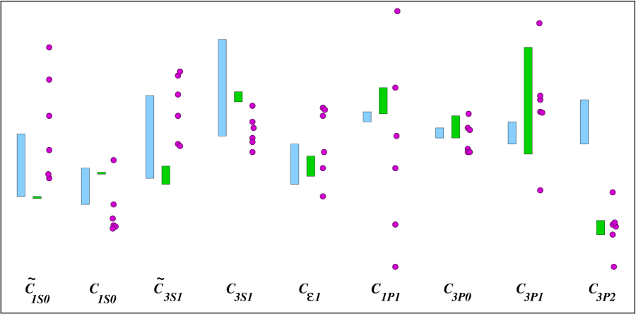
FIG. 3.: Graphical representation to compare the LECs determined in EFT with the values obtained from the various models. The left bar refers to NLO, the middle bar to NNLO and the filled circles to the various potentials discussed in the text. Note that the units are arbitrary, i.e. different scale factors (including in some cases an overall minus sign) have been assigned to the various LECs to obtain a more uniform representation.

REFERENCES

- [1] S. Weinberg, Phys. Lett. B251 (1990) 288; Nucl. Phys. B363 (1991) 3.
- [2] J. Gasser and H. Leutwyler, Nucl. Phys. B250 (1985) 465.
- [3] S. Myint and C. Rebbi, Nucl. Phys. B421 (1994) 241.
- [4] J. Heitger, R. Sommer and H. Wettig, Nucl. Phys. B588 (2000) 377.
- [5] G. Ecker et al., Nucl. Phys. B321 (1991) 311.
- [6] J.F. Donoghue, C. Ramirez and G. Valencia, Phys. Rev. D39 (1989) 1947.
- [7] S. Bellucci, J. Gasser and M.E. Sainio, Nucl. Phys. B423 (1994)80.
- [8] R. Baur and R. Urech, Nucl. Phys. B499 (1997) 319.
- [9] B. Moussallam, Nucl. Phys. B504 (1997) 381.
- [10] G. Ecker, J. Kambor and D. Wyler, Nucl. Phys. B394 (1993) 101.
- [11] V. Bernard, N. Kaiser and Ulf-G. Meißner, Nucl. Phys. A615 (1997) 483.
- [12] V. Bernard, N. Kaiser and Ulf-G. Meißner, Z. Phys. C70 (1996) 483; Phys. Lett. B378 (1996) 337.
- [13] B. Borasoy and Ulf-G. Meißner, Ann. Phys. (NY) 254 (1997) 192.
- [14] E. Epelbaum, W. Glöckle and Ulf-G. Meißner, Nucl. Phys. A671 (2000) 295.
- [15] C. Ordóñez, L. Ray and U. van Kolck, Phys. Rev. C53 (1996) 2086.
- [16] E. Epelbaoum, W. Glöckle and Ulf-G. Meißner, Nucl. Phys. A637 (1998) 107.
- [17] U. van Kolck, G.A. Miller and D.-O. Riska, Phys. Lett. B388 (1996) 679.
- [18] U. van Kolck, J.L. Friar and T. Goldman, Phys. Lett. B371 (1996) 169.
- [19] J.L. Friar, Few Body Syst. 22 (1997) 161.
- [20] P.G. Lepage, Lectures given at 9th Jorge Andre Swieca Summer School: Particles and Fields, Sao Paulo, Brazil, 16-28 Feb 1997 [hep-ph/9706029].
- [21] E. Epelbaum, doctoral thesis, published in Berichte des Forschungszentrum Jülich, No. 3803 (2000).
- [22] M.E. Luke and A.V. Manohar, Phys. Lett. B286 (1992) 348.
- [23] N. Kaiser, R. Brockmann and W. Weise, Nucl. Phys. A625 (1997) 758.
- [24] M.Walzl, Ulf-G. Meißner and E. Epelbaum, [nucl-th/0010019], Nucl. Phys. A (2001) in press.
- [25] E. Epelbaum et al., Phys. Rev. Lett. 86 (2001) 4787.
- [26] E. Epelbaum and Ulf-G. Meißner, Limit cycle behaviour of the chiral effective field theory potential for two nucleons, in preparation.
- [27] P. Büttiker and Ulf-G. Meißner, Nucl. Phys. A668 (2000) 97.
- [28] R. Machleidt, K. Holinde and Ch. Elster, Phys. Rep. 149 (1987) 1.
- [29] G. Janssen, K. Holinde and J. Speth, Phys. Rev. C54 (1996) 2218; K. Holinde, Prog. Part. Nucl. Phys. 66 (1996) 311.
- [30] E. Epelbaum, H. Kamada, A. Nogga, H. Witała, W. Glöckle, and Ulf-G. Meißner, in preparation.
- [31] R. Machleidt, Adv. Nucl. Phys. 19 (1989) 189.
- [32] V.G.J. Stoks et al., Phys. Rev. C49 (1994) 2950.
- [33] R. Machleidt, Phys. Rev. C63 (2001) 024001.
- [34] R.B. Wiringa et al., Phys. Rev. C51 (1995) 38.
- [35] P. Bedaque, H.W. Hammer and U. van Kolck, Phys. Rev. Lett. 82 (1999) 463.
- [36] S.R. Beane et al., [quant-ph/0010073].
- [37] E. Wigner, Phys. Rev. 51 (1937) 106; 51 (1937) 947; 56 (1939) 519.
- [38] D.B. Kaplan and M.J. Savage, Phys. Lett. B365 (1996) 244; D.B. Kaplan and A.V. Manohar, Phys. Rev. C56 (1997) 76.
- [39] T. Mehen, I.W. Stewart and M.B. Wise, Phys. Rev. Lett. 83 (1999) 931.