Range Corrections to Doublet S-Wave Neutron-Deuteron Scattering

Abstract

We calculate the range corrections to S-wave neutron-deuteron scattering in the doublet channel ($S=1/2$) to first order in $r/a$ where $a$ is the scattering length and $r$ the effective range. Ultraviolet divergences appearing at this order can be absorbed into a redefinition of the leading order three-body force. The corrections to the elastic scattering amplitude below the deuteron breakup threshold are computed. Inclusion of the range corrections gives good agreement with measured scattering data and potential model calculations.

There has been much interest recently in applying Effective Field Theory (EFT) methods to nuclear physics [1, 2, 3, 4]. EFT provides a framework in which to exploit the separation of scales in physical systems in order to perform systematic, model-independent calculations. For nuclear few-body systems, the long-distance scale is set by the large two-body scattering lengths, while the short-distance scale is set by the range of the nuclear force. The EFT includes long-distance physics explicitly, while corrections from short-distance physics are calculated perturbatively in an expansion in the ratio of these two scales. In the two-body system for small momenta ($p\stackrel{{\scriptstyle<}}{{{}_{\sim}}}m_{\pi}$), this program has been very successful and calculations of deuteron properties and electroweak processes have been carried out to $1\%$ accuracy (for a recent review, see Ref. [4]).

In the nuclear three-body system, considerable progress has been made as well. In most three-body channels, the two-body EFT can be extended in a straightforward way [5, 6, 7, 8]. However, the S-wave in the doublet channel ($S=1/2$) of neutron-deuteron scattering (with the triton as a three-body bound state) is more complicated and exhibits some surprising phenomena [9, 10, 11]. The renormalization of the three-body equations requires a one-parameter three-body force at leading order whose renormalization group evolution is governed by a limit cycle [12]. The variation of the three-body force parameter gives a compelling explanation of the Phillips line (an essentially equivalent explanation was previously given in Refs. [13, 14]). The phase shifts for S-wave neutron-deuteron scattering in the doublet channel have been studied at order $(r/a)^{0}$, where $a$ is the scattering length and $r$ the effective range [12]. In this paper, we calculate the linear corrections in $r/a$ to the elastic scattering phase shifts below the deuteron breakup threshold. The linear range corrections to the Phillips line have been studied in Ref. [14] using a different formalism.

Elastic neutron-deuteron scattering below the threshold of deuteron breakup can be described by an effective Lagrangian that includes only nucleons and has no explicit pions. For three-body calculations, it is convenient to use the dibaryon formalism of Ref. [15] in which auxiliary fields with baryon number two are introduced to represent two-nucleon states in a given partial wave. The effective Lagrangian for the nucleon-deuteron system is [12]

$${\cal L} = N^{\dagger}\bigg{(}i\partial_{0}+{\vec{\nabla}^{2}\over 2M}\bigg{)}N-t_{l}^{\dagger}\bigg{(}i\partial_{0}+\frac{\vec{\nabla}^{2}}{4M}-\Delta_{t}\bigg{)}t_{l}-s_{m}^{\dagger}\bigg{(}i\partial_{0}+{\vec{\nabla}^{2}\over 4M}-\Delta_{s}\bigg{)}s_{m}$$ (3)

$$-{g_{t}\over 2}\Big{(}t_{l}^{\dagger}N^{T}\tau_{2}\sigma_{l}\sigma_{2}N+\mbox{h.c.}\Big{)}-{g_{s}\over 2}\Big{(}s_{m}^{\dagger}N^{T}\sigma_{2}\tau_{m}\tau_{2}N+\mbox{h.c.}\Big{)}\,$$

$$-G_{3}\,N^{\dagger}\bigg{(}g_{t}^{2}(t_{l}\sigma_{l})^{\dagger}t_{l^{\prime}}\sigma_{l^{\prime}}+\frac{1}{3}\,g_{t}g_{s}\left[(t_{l}\sigma_{l})^{\dagger}s_{m}\tau_{m}+\mbox{h.c.}\right]+g_{s}^{2}(s_{m}\tau_{m})^{\dagger}s_{m^{\prime}}\tau_{m^{\prime}}\bigg{)}N+\ldots\,,$$

where $N$ represents the nucleon field and $t_{l}$ ($s_{m}$) are the dibaryon fields for the ${}^{3}S_{1}$ (${}^{1}S_{0}$) channels and carry spin (isospin) one, respectively. The dots indicate higher order terms with more fields/derivatives, which do not contribute to the order we are working. The first line in Eq. (3) contains the kinetic terms for the fields $N$, $t_{l}$, and $s_{m}$. The second line gives the coupling of the dibaryon fields to nucleon fields where $\sigma_{l}$ $(\tau_{m})$ are Pauli matrices acting in spin (isospin) space. Finally, the third line contains the three-body force. Note that this is the only three-body operator without derivatives that preserves spin and isospin symmetry [12, 16]. Other non-derivative three-body operators can be related to the one shown via Fierz transformations. Since the action is quadratic in the fields $t_{l}$ and $s_{m}$, it is straightforward to integrate them out and show that the theory is equivalent to one of nonrelativistic nucleons interacting via two-body and three-body contact interactions [7, 8, 12].

To obtain the exact dibaryon propagator, the bare propagator must be dressed by nucleon loops to all orders. This is illustrated in Fig. 1.

FIG. 1.: Geometric series leading to the exact dibaryon propagator. Double (single) lines represent bare dibaryon (nucleon) propagators, respectively.

The diagrams form a geometric series and are easily summed; the result is

$$iD_{j}(q_{0},\vec{q}\,) = {-i\;2\pi/(Mg_{j}^{2})\over-\gamma_{j}+\frac{1}{2}r_{j}\left(\gamma_{j}^{2}+Mq_{0}-\vec{q}^{\,2}/4\right)+\sqrt{-Mq_{0}+\vec{q}^{\,2}/4-i\epsilon}}\,,$$ (4)

where the subscript $j=t\,(s)$ for the ${}^{3}S_{1}\,(^{1}S_{0})$ channel. This propagator has a pole at $Mq_{0}-\vec{q}^{\,2}/4=-\gamma_{j}^{2}$, where $\gamma_{t}=45.68$ MeV and $\gamma_{s}=-7.88$ MeV. The effective ranges are $r_{t}=1.76$ fm and $r_{s}=2.75$ fm. These effective range parameters are related to the parameters appearing in the Lagrangian via

$${\gamma_{j}}={M^{2}g_{j}^{2}\over 4\pi}\left(1-\sqrt{1-{16\pi^{2}\Delta_{j}\over M^{3}g_{j}^{4}}}\;\right)\qquad\mbox{ and }\qquad r_{j}={4\pi\over M^{2}g_{j}^{2}}\,.$$ (5)

The scattering length $a_{j}$ is given by $-1/a_{j}=-\gamma_{j}+r_{j}\gamma_{j}^{2}/2$. Thus the Lagrangian of Eq. (3) reproduces the first two terms in the effective range expansion of the two-body scattering amplitude. Note that including the kinetic terms for the dibaryon fields in Eq. (3) is necessary to obtain the range correction.

The power counting in an EFT makes it possible to organize calculations in a systematic expansion in a small parameter. In the two-body sector, the power-counting scheme of [17, 18] takes $p\sim 1/a\sim Q$, where $p$ is the typical momentum of a nucleon and $1/a$ is the inverse scattering length. Note that $\gamma$ is $O(Q)$ as well since $\gamma=1/a+O(r/a^{2})$. The expansion parameter of the theory is $Q/\Lambda$, where $\Lambda$ represents the scale where short-distance physics becomes important. For systems interacting via short-range interactions, the effective range is expected to be set by $\Lambda$. So the expansion parameter is $Q/\Lambda\sim r/a\approx\gamma r$. The leading order term in the expansion of the two-body scattering amplitude is $O(Q^{-1})$. If we integrate out the dibaryon fields, the two-body operators without derivatives are treated nonperturbatively because the renormalization group equations dictate that their coefficients are $O(Q^{-1})$. In the dibaryon formalism, $2\pi\Delta/(Mg^{2})=1/a\sim Q$, which requires summing the bubbles in Fig. 1. At leading order in $Q$, the theory reproduces Eq. (4) in the limit $r_{t},r_{s}\rightarrow 0$. The two-body operators with two spatial derivatives or one time derivative which are given by the kinetic terms of the dibaryon fields appear at next-to-leading order in the $Q$ expansion, giving a contribution of $O(Q^{0})$ to the scattering amplitude. When these operators are included in the three-body problem, they also give a correction that is suppressed by one power of $Q$ relative to the leading order. Since the coefficients of these operators are proportional to the two-body effective ranges, we refer to these corrections as effective range corrections.

Next we consider power counting in the three-body sector. EFT power counting shows that all diagrams that contain only non-derivative contact interactions are $O(Q^{-2})$ [12]. These diagrams can be summed using the integral equation shown in Fig. 2. At this order in the EFT, it is appropriate to use the propagator of Eq. (4) in the limit $r_{t},r_{s}\to 0$.

FIG. 2.: Leading order integral equation. Shaded (full) double lines indicate spin-triplet (spin-singlet) dibaryon. Single line indicates nucleon propagator.

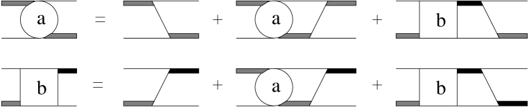
However, it turns out that the resulting integral equation has no unique solution if the cutoff $\Lambda$ is taken to infinity [13, 19]. If the integral equation is regularized with a finite cutoff $\Lambda$, the solution displays a strong cutoff dependence. The integral equation can be renormalized by absorbing the cutoff dependence into the three-body force of Eq. (3) [12]. The diagrams with the three-body force are naively $O(Q^{0})$. However, in the $S=1/2$ channel, the leading three-body operator with no derivatives is relevant at low energies because the renormalization group evolution enhances the coefficient $G_{3}$ in Eq. (3) to $O(Q^{-2})$ rather than $O(Q^{0})$ as naively expected [12]. It is convenient to pull out a factor of $2M/\Lambda^{2}$ and define $G_{3}(\Lambda)=2MH(\Lambda)/\Lambda^{2}$ with

$$H(\Lambda)=-\frac{\sin[s_{0}\ln({\Lambda}/{\Lambda_{*}})-{\rm arctg}(1/s_{0})]}{\sin[s_{0}\ln({\Lambda}/{\Lambda_{*}})+{\rm arctg}(1/s_{0})]}\,,$$ (6)

where $s_{0}\approx 1.0064$ is determined by the asymptotic behavior of the integral equation and $\Lambda_{*}$ is the three-body force parameter [12, 20]. As a consequence, there are certain cutoffs for which the three-body force vanishes. Since all observables are independent of the cutoff, it is possible to obtain a renormalized equation by choosing a cutoff with vanishing three-body force [21]. The parameter $\Lambda_{*}$ then appears in the upper limit of the integral. Evaluating the diagrams in Fig. 2, the renormalized equation in the limit $r_{t},r_{s}\to 0$ takes the form [12, 19]

$$2{-\gamma_{t}+\sqrt{3p^{2}/4-ME_{k}}\over p^{2}-k^{2}}a^{0}_{k}(p)=K_{k}(p,k)+{2\over\pi}\int_{0}^{\Lambda_{n}(\Lambda_{*})}\!\!\!\!\!\!\!dq{q^{2}\,{\cal P}\over q^{2}-k^{2}}K_{k}(p,q)\bigg{(}a^{0}_{k}(q)+3b^{0}_{k}(q)\bigg{)}$$ (7)

$$2{-\gamma_{s}+\sqrt{3p^{2}/4-ME_{k}}\over p^{2}-k^{2}}b^{0}_{k}(p)=3K_{k}(p,k)+{2\over\pi}\int_{0}^{\Lambda_{n}(\Lambda_{*})}\!\!\!\!\!\!\!dq{q^{2}\,{\cal P}\over q^{2}-k^{2}}K_{k}(p,q)\bigg{(}3a^{0}_{k}(q)+b^{0}_{k}(q)\bigg{)}\,,$$ (8)

where $k$ $(p)$ denote the incoming (outgoing) momenta in the center-of-mass frame, $ME_{k}=3k^{2}/4-\gamma_{t}^{2}$ is the total energy, and $\Lambda_{n}=\Lambda_{*}\exp[(n\pi+\arctan(1/s_{0}))/s_{0}]$ with $n$ a natural number. Three-body observables are independent of $n$ up to corrections that are suppressed by inverse powers of $\Lambda_{n}$ [21]. The kernel $K_{k}(p,q)$ arises from the S-wave projected one-nucleon exchange and is given by

$$K_{k}(p,q)={1\over 2pq}\ln\left({q^{2}+pq+p^{2}-ME_{k}\over q^{2}-pq+p^{2}-ME_{k}}\right)\,.$$ (9)

The amplitude $a^{0}_{k}(p)$ is normalized such that $a^{0}_{k}(k)=1/(k\cot\delta)$ with $\delta$ the elastic scattering phase shift.

Recently, various authors have suggested treating range corrections nonperturbatively in both the two- and three-body systems [22, 23, 24, 25, 26]. This can be motivated by arguing that a nonperturbative treatment of range corrections resums large corrections proportional to $(\gamma_{t}r_{t})^{n}$ to all orders in $n$. Since $\gamma_{t}r_{t}\approx 0.4$, these corrections can be numerically important despite being formally subleading in the $Q$ expansion[25]. Alternatively, one can imagine a power counting in which $r$ is $O(Q^{-1})$ [22, 23, 24, 25]. In the two-body sector, such a power counting was shown to simplify calculations and improve the convergence of the expansion [25]. Furthermore, the coefficients of higher derivative S-wave operators are no longer enhanced by renormalization group evolution and naive dimensional analysis can be used to estimate their contribution to amplitudes.

A nonperturbative treatment of range corrections in the three-body problem was studied in Refs. [26, 27]. The integral equation of Fig. 2 is solved using the propagator of Eq. (4) without expanding in $r$. This drastically changes the nature of the solution to the integral equation. Since the dibaryon propagator falls as $1/q^{2}$ rather than $1/q$ for large $q$, the kernel is damped at large loop momenta, and the integral equation has a unique solution even in the absence of the three-body force. The three-body force is not enhanced by renormalization and is a subleading effect suppressed by $Q^{2}$. There is no three-body parameter in the leading order calculation and therefore no Phillips line. Surprisingly, the Phillips line is not even recovered at $O(Q^{0})$, when the three-body force is included. In Ref. [26], it was shown that when the range is treated nonperturbatively and the cutoff, $\Lambda$, is taken to infinity, the solution is completely insensitive to the numerical value of the three-body force. Furthermore, the obtained scattering phase shifts strongly disagree with experiment [26].

It is not clear why the nonperturbative treatment of the range corrections fails. One possible problem is that the dibaryon propagators have spurious poles at $Mq_{0}-\vec{q}^{\,2}/4=2/r+O(\gamma r)$. These poles can be avoided by using a momentum cutoff in the range $\gamma<\Lambda\leq 1/r$. The three-body force can be tuned in such a way as to leave results approximately cutoff independent when the cutoff is varied within this window. Unfortunately, since $a_{t}\approx 3\,r_{t}$, unreasonably small cutoffs must be used in this method. Moreover, the nonperturbative range correction worsens the agreement with the Phillips line.

In the present paper, we take a different approach and compute the range corrections to $a^{0}_{k}(k)$ perturbatively, working to $O(Q^{-1})$. An important question is whether higher derivative three-body operators also contribute at this order. These operators will include at least one time derivative or two spatial derivatives and hence contribute to the amplitude at $O(Q^{2})$, according to naive dimensional analysis. This is much higher order than the range correction to the three-body amplitude, which is $O(Q^{-1})$. Higher derivative three-body operators could only contribute at this order if there were a renormalization group enhancement of their coefficients, which is not the case. Consequently, the range correction is the only contribution at this order. In the following, it is more convenient to label the contributions by powers of $\gamma r$ relative to the leading order. The linear range correction is then $O(\gamma r)$. Below, it is demonstrated that the range correction can be calculated without introducing any terms not already present in Eq. (3). The operator which renormalizes the leading order calculation can also be used to renormalize the loop graphs that appear at $O(\gamma r)$. However, the running of the coefficient $H(\Lambda)$ needs to be modified.

Since the computation of the range corrections requires no additional counterterms, only the two-body effective ranges $r_{t}$ and $r_{s}$ enter as new parameters at this order of the calculation. The only parameter to be fixed from a three-body datum is the three-body force parameter, $\Lambda_{*}$. For example, if $\Lambda_{*}$ is fixed to reproduce the observed neutron-deuteron scattering length, the energy dependence of the scattering amplitude is completely predicted up to corrections of $O((\gamma r)^{2})$.

To calculate the range corrections it is convenient to formally expand the amplitudes $a_{k}(p)$, $b_{k}(p)$ and the three-body force $H(\Lambda)$ in powers of $\gamma r$,

$$a(q)=a_{k}^{0}(q)+a_{k}^{1}(q)+...\,,$$ (10)

$$b(q)=b_{k}^{0}(q)+b_{k}^{1}(q)+...\,,$$ (11)

$$H(\Lambda)=H^{0}(\Lambda)+H^{1}(\Lambda)+...\,,$$ (12)

where the superscript denotes the power of $\gamma r$. The amplitudes $a_{k}^{0}(q)$ and $b_{k}^{0}(q)$ are the solutions of Eq. (7) and $H^{0}(\Lambda)$ is given in Eq. (6). In the following, we will calculate $a_{k}^{1}(k)$ and obtain the renormalization group evolution of $H^{1}(\Lambda)$.

The Feynman diagrams contributing to $a^{1}_{k}(k)$ are shown in Fig. 3.

FIG. 3.: Feynman diagrams for range correction. (a) Range correction: double line with cross denotes $O(\gamma r)$ piece of the dibaryon propagator. (b) Subleading three-body force: filled square denotes insertion of $H^{1}(\Lambda)$. The propagators are as in Fig. 2. Not shown are diagrams that vanish as $\Lambda\to\infty$.

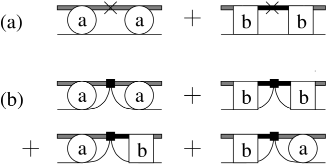
Fig. 3(a) shows the diagrams from the range correction. The double lines with the cross denote the $O(\gamma r)$ piece of the dibaryon propagator, $\widetilde{D}_{j}(q_{0},\vec{q}\,)$. Expanding Eq. (4) in $r_{j}$, we obtain the Feynman rule

$$i\widetilde{D}_{j}(q_{0},\vec{q}\,) = {-2\pi i\over Mg_{j}^{2}}\;{r_{j}\over 2}{\left(\vec{q}^{\,2}/4-Mq_{0}-\gamma_{j}^{2}\right)\over\left(-\gamma_{j}+\sqrt{-Mq_{0}+\vec{q}^{\,2}/4-i\epsilon}\right)^{2}}\,$$ (13)

$$= {-2\pi i\over Mg_{j}^{2}}\left({\gamma_{j}r_{j}\over-\gamma_{j}+\sqrt{-Mq_{0}+\vec{q}^{\,2}/4-i\epsilon}}+{r_{j}\over 2}\right)\,.$$ (14)

In order to evaluate the Feynman diagrams in Fig. 3(a), it is convenient to use the form given in the second line of Eq. (13). The constant term in Eq. (13) does not contribute because the contour integral over the zero component of the loop momentum can be evaluated without enclosing a singularity [20]. Fig. 3(b) gives the contribution of the subleading piece of the three-body force, $H^{1}(\Lambda)$. In addition to the diagrams shown in Fig. 3(b), there are four more diagrams where the $H^{1}(\Lambda)$ insertion is dressed on only one side by either $a^{0}_{k}(q)$ or $b^{0}_{k}(q)$ and a diagram with the undressed $H^{1}(\Lambda)$. These diagrams are also included in the calculation, but it is shown below that their contribution vanishes as $\Lambda\to\infty$.

The evaluation of these diagrams is straightforward. After projecting onto the S-waves, we obtain:

$$a^{1}_{k}(k) = \gamma_{t}r_{t}\,a^{0}_{k}(k)+\gamma_{t}{2\over\pi}\int_{0}^{\Lambda_{n}(\Lambda_{*})}dq\frac{q^{2}\,{\cal P}}{q^{2}-k^{2}}\,\frac{2\gamma_{t}r_{t}\;a^{0}_{k}(q)^{2}}{\gamma_{t}+\sqrt{3q^{2}/4-ME_{k}}}$$ (17)

$$+\gamma_{t}{2\over\pi}\int_{0}^{\Lambda_{n}(\Lambda_{*})}dq\frac{q^{2}\;b^{0}_{k}(q)^{2}}{(q^{2}-k^{2})^{2}}\;\frac{8}{3}\gamma_{s}r_{s}\left(-\gamma_{s}+\sqrt{3q^{2}/4-ME_{k}}\right)$$

$$+{8\gamma_{t}\over 3}{H^{1}(\Lambda_{n})\over\Lambda_{n}^{2}}\left[1+{2\over\pi}\int_{0}^{\Lambda_{n}(\Lambda_{*})}dq{q^{2}\,{\cal P}\over q^{2}-k^{2}}\bigg{(}a^{0}_{k}(q)+b^{0}_{k}(q)\bigg{)}\right]^{2}\,.$$

Note that for the integral in the second line no principal value prescription is required since $b^{0}_{k}(k)=0$.

There are four contributions to the $O(\gamma r)$ corrections to the amplitude. First, the residue of the pole in the deuteron propagator changes by a factor $1+\gamma_{t}r_{t}$. This changes the LSZ factor that goes into the leading-order calculation, giving rise to the first term in Eq. (17). The second and third terms in Eq. (17) come from the diagrams in Fig. 3(a). The fourth term comes from diagrams involving the subleading piece of the three-body force, $H^{1}(\Lambda)$.

In order to determine $H^{1}(\Lambda)$, it is necessary to know the large $\Lambda$ dependence of the integrals in Eq. (17). Since the combination $a^{0}_{k}(q)-b^{0}_{k}(q)$ falls off sufficiently fast for large $q$ (cf. Ref. [12]), only the asymptotic form of the combination $a^{0}_{k}(q)+b^{0}_{k}(q)$ for $q\gg\gamma$ is needed:

$$a^{0}_{k}(q)+b^{0}_{k}(q)\rightarrow s_{k}(q)={\cal N}(k)\cos(s_{0}\ln(q/\Lambda_{*})+\delta)\,,$$ (18)

where we have suppressed the dependence of ${\cal N}(k)$ on $\Lambda$ and $\gamma$. It is especially important to note that the phase of $s_{k}(q)$ is independent of $k$ so $s_{k}(q)$ factorizes into a product of an unknown function of $k$ and a known function of $q$. This will allow us to determine $H^{1}(\Lambda)$ analytically and show that all divergences in the range correction are cancelled by this counterterm.

Inserting Eq. (18) into Eq. (17) gives the divergent piece of the range correction

$$\delta a_{\rm div}={2\gamma_{t}\over\pi}\left({\gamma_{t}r_{t}+\gamma_{s}r_{s}\over\sqrt{3}}\int^{\Lambda}{dq\over q}s^{2}_{k}(q)+{16\over 3\pi}{H^{1}(\Lambda)\over\Lambda^{2}}\left[\int^{\Lambda}dqs_{k}(q)\right]^{2}\right)\,.$$ (19)

The divergence is cancelled if

$${H^{1}(\Lambda)\over\Lambda^{2}} = -{\sqrt{3}\pi\over 16}(\gamma_{t}r_{t}+\gamma_{s}r_{s}){\int^{\Lambda}dqs^{2}_{k}(q)/q\over[\int^{\Lambda}dqs_{k}(q)]^{2}}$$ (20)

$$= -{\sqrt{3}\pi\over 16}(\gamma_{t}r_{t}+\gamma_{s}r_{s}){(1+s_{0}^{2})^{2}\over 4s_{0}\Lambda^{2}}{2s_{0}\ln(\Lambda/\Lambda_{*})+2\delta+\sin(2s_{0}\ln(\Lambda/\Lambda_{*})+2\delta)\over[\cos(s_{0}\ln(\Lambda/\Lambda_{*})+\delta)+s_{0}\sin(s_{0}\ln(\Lambda/\Lambda_{*})+\delta)]^{2}}$$ (21)

$$\equiv -{\sqrt{3}\pi\over 16}(\gamma_{t}r_{t}+\gamma_{s}r_{s}){F(\Lambda)\over\Lambda^{2}}\,,$$ (22)

where the last line defines $F(\Lambda)$. Note that $H^{1}(\Lambda)$ is the coefficient of an operator with no derivatives and cannot be a function of $k$. As required, all $k$ dependence has cancelled in the expression for $H^{1}(\Lambda)$. Furthermore, $H^{1}(\Lambda)/\Lambda^{2}$ scales like $1/\Lambda^{2}$ (up to logarithmic corrections) for large $\Lambda$. In the third line of Eq. (17), it is only necessary to keep the term in which $H^{1}(\Lambda)$ is multiplied by two linearly divergent integrals. This term corresponds to the diagrams shown in Fig. 3(b). The other terms can be discarded since their contribution can be made arbitrarily small by choosing an appropriate value for $\Lambda$. Thus the renormalized expression for the range correction is

$$a^{1}_{k}(k) = \gamma_{t}r_{t}\,a^{0}_{k}(k)+\gamma_{t}{2\over\pi}\int_{0}^{\Lambda_{n}(\Lambda_{*})}dq\frac{q^{2}\,{\cal P}}{q^{2}-k^{2}}\,\frac{2\gamma_{t}r_{t}\;a^{0}_{k}(q)^{2}}{\gamma_{t}+\sqrt{3q^{2}/4-ME_{k}}}$$ (25)

$$+\gamma_{t}{2\over\pi}\int_{0}^{\Lambda_{n}(\Lambda_{*})}dq\frac{q^{2}\;b^{0}_{k}(q)^{2}}{(q^{2}-k^{2})^{2}}\;\frac{8}{3}\gamma_{s}r_{s}\left(-\gamma_{s}+\sqrt{3q^{2}/4-ME_{k}}\right)$$

$$-{2\gamma_{t}\over\sqrt{3}\pi}(\gamma_{t}r_{t}+\gamma_{s}r_{s}){F(\Lambda_{n})\over\Lambda_{n}^{2}}\left[\int_{0}^{\Lambda_{n}(\Lambda_{*})}dq\bigg{(}a^{0}_{k}(q)+b^{0}_{k}(q)\bigg{)}\right]^{2}\,.$$

The above expression is cutoff independent (up to corrections of $O(1/\Lambda_{n})$). Note the function $F(\Lambda)$ is known analytically but depends on the asymptotic phase $\delta$, which must be determined numerically by fitting to the leading-order solution $a^{0}_{k}(q)+b^{0}_{k}(q)$.

In Fig. 4, we show our result for $k\cot\delta$. The leading-order (LO) calculation is indicated by the full line, while the next-to-leading-order (NLO) calculation is given by the dashed line. At each order, $\Lambda_{*}$ is tuned to produce the measured neutron-deuteron scattering length, $a_{nd}^{(1/2)}=(0.65\pm 0.04)$ fm [28]. We find $\Lambda_{*}^{LO}=3.6\,\gamma_{t}=0.83\,\rm{fm}^{-1}$ and $\Lambda_{*}^{NLO}=4.1\,\gamma_{t}=0.95\,\rm{fm}^{-1}$.

FIG. 4.: Results for $k\cot\delta$: LO (NLO) calculation is indicated by solid (dashed) line. Triangle gives the experimental value of the scattering length from Ref. [28], circles show the phase shift analysis of Ref. [29], and squares show the potential model calculation of Ref. [30].

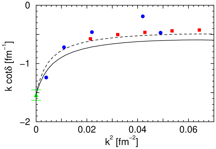
In Fig. 4, the circles correspond to the phase shift analysis of Ref. [29], while the squares show a potential model calculation using the Argonne V18 nucleon-nucleon potential and the Urbana three-nucleon force [30]. The triangle gives the experimental value of the $nd$-scattering length from Ref. [28]. The range corrections are small all the way up to the breakup threshold. It is encouraging to see that the perturbative corrections are small even though $\gamma_{t}r_{t}\approx 0.4$ is not a very small expansion parameter. This suggests that the EFT expansion is well behaved. The range correction clearly improves agreement with the phase shift analysis of Ref. [29]. Note that this phase shift analysis is more than 30 years old and gives no error estimates. The errors of the analysis are at least as large as the error of the scattering length; most likely they are larger. Consequently, it is more meaningful to compare to the potential model calculation of [30], which agrees well with the NLO result.

In summary, we have calculated the S-wave phase shifts for neutron-deuteron scattering in the doublet channel to $O(\gamma r)$ and found good agreement with available data. We have shown that the corrections at this order can be renormalized by modifying the running of the leading order three-body force. Apart from the two-body effective ranges $r_{t}$ and $r_{s}$, no new parameters enter at this order. In Refs. [7, 8], it was shown that the perturbative treatment of the range corrections in other channels where three-body forces are subleading gives good agreement with available data as well. As stated earlier, Ref. [14] has calculated the Phillips line to $O(\gamma r)$ and obtained results which agree well with the Phillips line obtained from various potential models. Furthermore, if one demands that the neutron-deuteron scattering length be correctly reproduced, then the Phillips line predicts the triton binding energy. The prediction is $8.0$ MeV at $O((\gamma r)^{0})$ [12, 14] and $8.8$ MeV at $O(\gamma r)$ [14]. These numbers compare well with the measured binding energy of $8.5$ MeV, and again the range corrections improve agreement with experiment. Together, these results show that the power counting of [17, 18] is adequate for three-body nuclear systems at very low energies. This suggests that the perturbative method could be used for precise calculations of phenomenologically important three-body processes such as polarization observables in neutron-deuteron scattering and the $\beta$-decay of the triton.

We acknowledge useful discussions with P. Bedaque, E. Braaten, R.J. Furnstahl, R. Perry, and M. Strickland. This work was supported by the National Science Foundation under Grant No. PHY–9800964.

REFERENCES

- [1] Proceedings of the Joint Caltech/INT Workshop: Nuclear Physics with Effective Field Theory, ed. R. Seki, U. van Kolck, and M.J. Savage (World Scientific, 1998).
- [2] Proceedings of the INT Workshop: Nuclear Physics with Effective Field Theory II, ed. P.F. Bedaque, M.J. Savage, R. Seki, and U. van Kolck (World Scientific, 2000).
- [3] U. van Kolck, Prog. Part. Nucl. Phys. 43 (1999) 337.
-
[4]
S.R. Beane, P.F. Bedaque, W.C. Haxton, D.R. Phillips,
and M.J. Savage,
[nucl-th/0008064]. - [5] P.F. Bedaque and U. van Kolck, Phys. Lett. B 428 (1998) 221.
- [6] P.F. Bedaque, H.-W. Hammer, and U. van Kolck, Phys. Rev. C 58 (1998) R641.
- [7] P.F. Bedaque and H.W. Grießhammer, Nucl. Phys. A 671 (2000) 357.
- [8] F. Gabbiani, P.F. Bedaque, and H.W. Grießhammer, Nucl. Phys. A 675 (2000) 601.
- [9] L.H. Thomas, Phys. Rev. 47 (1935) 903.
- [10] V.N. Efimov, Sov. J. Nucl. Phys. 12 (1971) 589.
- [11] A.C. Phillips, Nucl. Phys. A 107 (1968) 209.
- [12] P.F. Bedaque, H.-W. Hammer, and U. van Kolck, Nucl. Phys. A 676 (2000) 357.
- [13] G.S. Danilov, Sov. Phys. JETP 13 (1961) 349; G.S. Danilov and V.I. Lebedev, Sov. Phys. JETP 17 (1963) 1015.
- [14] V. Efimov and E.G. Tkachenko, Phys. Lett. B 157 (1985) 108; Sov. J. Nucl. Phys. 47 (1988) 17; Few Body Syst. 4 (1988) 71.
- [15] D. B. Kaplan, Nucl. Phys. B 494 (1997) 471.
- [16] T. Mehen, I.W. Stewart, and M.B. Wise, Phys. Rev. Lett. 83 (1999) 931.
- [17] D.B. Kaplan, M. J. Savage, and M.B. Wise, Phys. Lett. B 424 (1998) 390; Nucl. Phys. B 534 (1998) 329.
- [18] U. van Kolck, Nucl. Phys. A 645 (1999) 273.
- [19] G.V. Skorniakov and K.A. Ter-Martirosian, Sov. Phys. JETP 4 (1957) 648.
- [20] P.F. Bedaque, H.-W. Hammer, and U. van Kolck, Nucl. Phys. A 646 (1999) 444; Phys. Rev. Lett. 82 (1999) 463.
- [21] H.-W. Hammer and T. Mehen, Nucl. Phys. A (in print), [nucl-th/0011024].
- [22] T. D. Cohen, in Ref. [2], [nucl-th/9904052].
- [23] T. D. Cohen and J. M. Hansen, Phys. Rev. C 59 (1999) 3047.
- [24] D. B. Kaplan and J. V. Steele, Phys. Rev. C 60 (1999) 064002.
- [25] S. R. Beane and M. J. Savage, [nucl-th/0011067].
- [26] F. Gabbiani, [nucl-th/0104088].
- [27] I.V. Simenog and D.V. Shapoval, Sov. J. Nucl. Phys. 47 (1988) 620.
- [28] W. Dilg, L. Koester and W. Nistler, Phys. Lett. B 36 (1971) 208.
- [29] W. T. H. van Oers, J. D. Seagrave, Phys. Lett. B 24 (1967) 562.
- [30] A. Kievsky, S. Rosati, W. Tornow, and M. Viviani, Nucl. Phys. A 607 (1996) 402.