Antibaryon production in hot and dense nuclear matter

Abstract

The production of antibaryons is calculated in a microscopic transport approach employing multiple meson fusion reactions according to detailed balance relations with respect to baryon-antibaryon annihilation. It is found that the abundancies of antiprotons as observed from peripheral to central collisions of $Pb+Pb$ at the SPS and $Au+Au$ at the AGS can approximately be described on the basis of multiple interactions of ’formed’ hadronic states which drive the system to chemical equilibrium by flavor exchange or quark rearrangement reactions.

PACS: 24.10.-i; 24.10.Cn; 24.10.Jv; 25.75.-q; 14.65.-q

Keywords: Nuclear reaction models and methods; Many-body theory; Relativistic models; Relativistic heavy-ion collisions; Quarks

1 Introduction

Ever since the first observation of antiproton production in proton-nucleus [1, 2, 3] and nucleus-nucleus collisions [4, 5, 6, 7, 8] the production mechanism has been quite a matter of debate. Especially in nucleus-nucleus collisions at subthreshold energies traditional cascade calculations, that employ free $NN$ production and $\bar{p}N$ annihilation cross sections, essentially fail in describing the high cross sections seen from 1.5 - 2.1 A$\cdot$GeV [9, 10, 11]. Thus multiparticle nucleon interactions [12, 13] have been suggested as a possible solution to this problem. On the other hand it has been pointed out that the quasi-particle properties of the nucleons and antinucleons might be important for the $\bar{p}$ production process which become more significant with increasing nuclear density. Schaffner et al. [14] found in a static thermal relativistic model based on scalar and vector self energies– assuming kinetic and chemical equilibrium – that the $\bar{p}$-abundancy might be dramatically enhanced when assuming the antiproton self energy in the medium to be given by charge conjugation of the nucleon self energy. This assumption implies strong attractive vector self energies for the antiprotons which lead to a reduction of the necessary energy to produce $p\bar{p}$ pairs in the medium by binary quasi-particle interactions. On the other hand, such self energies will lead to different spectral slopes of protons and antiprotons as pointed out in Ref. [15].

First nonequilibrium calculations within a fully relativistic transport model for antiproton production – including $\bar{p}$ annihilation as well as the change of the quasi-particle properties in the medium – have been performed in Ref. [10]. There it was found that according to the reduced antinucleon energy in the medium the threshold for $\bar{p}$-production is shifted to lower energy and the antiproton cross section prior to annihilation becomes enhanced e.g. for $Si+Si$ at 2.1 GeV$\cdot$GeV by approximately a factor 70 as compared to a relativistic cascade calculation where no in-medium effects are incorporated. Later on, a couple of relativistic transport calculations have been performed [16, 17, 18, 19] essentially pointing out that all the low energy data from proton-nucleus and nucleus-nucleus collisions are compatible with attractive $\bar{p}$ self energies (at normal nuclear matter density $\rho_{0}$) in the order of -100 to -150 MeV [19, 20, 21]. However, it had been stressed at that time that the high antiproton yield might also be attributed to mesonic production channels [22, 23, 24] since $p\bar{p}$ annihilation leads to multi-pion final states with an average abundancy of 5 pions [25], which e.g. might stem from an intermediate state of 2 $\rho$-mesons and a pion.

With new data coming up on antibaryon production from nucleus-nucleus collisions at the AGS [26, 27, 28] and SPS [29, 30, 31, 32, 33] the $\bar{p},\bar{\Lambda}$ enhancement factors seen experimentally were no longer that dramatic as at SIS energies, however, traditional cascade calculations employing free production and annihilation cross sections again were not able to reproduce the measured abundancies and spectra [34, 35, 36, 37, 38] especially for $\Xi,\bar{\Xi}$ and $\Omega,\bar{\Omega}$. Here additional collective mechanisms in the entrance channel have been suggested such as color rope formation [39] or hot plasma droplet formation [40]. In another language this has been addressed also as string fusion [41, 42], a precursor phenomenon for the formation of a quark-gluon plasma (QGP).

The intimate connection of antibaryon abundancies with the possible observation of a new state of the strongly interacting hadronic matter, i.e. the quark-gluon plasma, has been often discussed since the early suggestion in Ref. [43] that especially the enhanced yield of strange antibaryons – approximately in chemical equilibrium with the other hadronic states – should be a reliable indicator for a new state of matter. In fact, the data on strange baryon and antibaryon production from the NA49 and WA97 Collaborations show an approximate chemical equilibrium [44, 45, 46, 47] with an enhancement of the $\Omega^{-},\Omega^{+}$ yield in central $Pb+Pb$ collisions (per participant) relative to $pBe$ collisions at the same invariant energy per nucleon by a factor $\sim$ 15. As pointed out in Ref. [48] the data on multi-strange antibaryons at the SPS seem compatible with a canonical ensemble in chemical equilibrium. At AGS energies of 11.6 A$\cdot$GeV/c, furthermore, a high ratio of $\bar{\Lambda}$/$\bar{p}$ of $3.6^{+4.7}_{-1.8}$ has been reported [28] for central collisions of $Au+Au$, that is not described by any approach so far. Strange flavor exchange reactions [49] help in creating multistrange antibaryons, however, the latter strangeness enhancement factors could not be described within traditional transport or cascade simulations without additional assumptions such as enhanced string tensions or reduced quark masses [37].

In a more recent paper Rapp and Shuryak have taken up again the idea of multi-meson production channels for baryon-antibaryon pairs [50] to describe the antiproton abundancies in central $Pb+Pb$ collisions at the SPS by introducing additionally a finite pion chemical potential which helps in enhancing the multi-pion collision rate. Later on, Greiner and Leupold [51] have applied the same concept for the $\bar{\Lambda}$ production by a couple of mesons including a $K^{+}$ or $K^{0}$ (for the $\bar{s}$ quark). However, such estimates remain schematic unless fully microscopic multi-particle calculations support or disprove such suggestions. The problem here is that most of the transport models include only binary reactions in the entrance channel whereas the final channel of an energetic collision may well consist of many hadrons emerging from the decay of strings that are excited in the initial reaction. Thus, as has been pointed out quite often [50, 52, 53], detailed balance is not included on the many-particle level leading to an improper equilibrium state for large times ($t\rightarrow\infty$).

In this work we will address two separate questions: the first one is of more formal nature and related to a transport approach that properly takes into account reactions of 2 hadrons $\rightarrow n$ hadrons and vice versa employing detailed balance (Section 2). The second one addresses a suitable covariant scheme for the calculation of such multi-particle reactions in transport models. The method and its implementation in the hadron-string-dynamics (HSD) transport approach [20, 54] will be described in Section 3. A first application of this novel approach is devoted to the problem of antibaryon production in relativistic nucleus-nucleus collisions by multi-meson reaction channels. Respective calculations and studies at SPS and AGS energies – with a focus on antiproton abundancies – will be presented in Section 4 whereas Section 5 concludes this work with a summary.

2 Generalized transport equations

In this Section a brief description of the relativistic transport model is given with emphasis on a new development, i.e. the multi-particle reaction dynamics. First we summarize (or review) the relevant equations determining the dynamics of baryons and mesons and then discuss a flavor rearrangement model for baryon-antibaryon annihilation and production in the extended HSD transport approach.

2.1 Hadron transport and multi-particle transitions

Since the covariant transport approach for binary reactions has been extensively discussed in Refs. [55] and in the reviews [20, 56, 58] we only recall the basic equations that are relevant for a proper understanding of the results to be reported in this study.

For the discussion of the general collision terms the hadron self energies will be discarded for transparency, such that the transport equation in the cascade limit reduces to

$$p_{\mu}\partial^{\mu}_{x}F_{i}(x,p)=(p_{0}\partial_{t}+{\vec{p}}\cdot{\vec{\partial}}_{r})F_{i}(x,p)=I_{coll}^{i},$$ (1)

where $F_{i}(x,p)$ is the Lorentz covariant 8 dimensional phase-space distribution function for an off-shell hadron with quantum numbers $i$, i.e.

$$F(x,p)=A(x,p)f(x,p),$$ (2)

where $A(x,p)$ denotes the hadron spectral function while $f(x,p)$ describes the occupation probability in phase-space. The off-shell propagation of hadrons leads to additional terms in the l.h.s. of (1) that describe the change of the spectral function $A_{i}(x,p)$ during the propagation. These terms are omitted here since the actual calculations will be performed in the on-shell limit. For details on the off-shell propagation of hadrons in the medium the reader is referred to Refs. [59, 60].

We now turn to a discussion of the collision term $I_{coll}^{i}$, which includes the new elements to be presented below. In the most general case it is a sum of collision integrals involving $n\leftrightarrow m$ reactions,

$$I_{coll}=\sum_{n}\sum_{m}\ I_{coll}[n\leftrightarrow m].$$ (3)

The general form for off-shell fermions with spectral functions $A_{i}(x,p_{i})$ in case of 2-body interactions is given by [59]

$$I_{coll}^{i}[2\leftrightarrow 2]=$$ (4)

$$\frac{1}{2}\sum_{j}\sum_{k,l}\frac{1}{(2\pi)^{12}}\int d^{4}p_{2}\,d^{4}p_{3}\,d^{4}p_{4}\ A_{i}(x,p)A_{j}(x,p_{2})A_{k}(x,p_{3})A_{l}(x,p_{4})$$

$$\times W_{2,2}(p,p_{2};i,j\mid p_{3},p_{4};k,l)\ (2\pi)^{4}\ \delta^{4}(p^{\mu}+p^{\mu}_{2}-p_{3}^{\mu}-p_{4}^{\mu})$$

$$\times[f_{k}(x,p_{3})f_{l}(x,p_{4})(1-f_{i}(x,p))(1-f_{j}(x,p_{2}))$$

$$-f_{i}(x,p)f_{j}(x,p_{2})(1-f_{k}(x,p_{3}))(1-f_{l}(x,p_{4}))].$$

This collision integral describes the change in the 8 dimensional phase-space distribution function $F_{i}(x,p)$ due to the collisions of two baryons with momenta $p^{\mu}$ and $p^{\mu}_{2}$ and discrete quantum numbers $i$ and $j$, respectively, whereas the two fermions in the final state of the reaction are labeled by their momenta $p_{3}$ and $p_{4}$ and discrete quantum numbers $k$ and $l$. The $\delta-$function guarantees energy and momentum conservation in the individual collision while $W_{2,2}(p,p_{2};i,j\mid p_{3},p_{4};k,l)$ denotes the transition probability (or transition amplitude squared) for this reaction which in case of fermions includes the antisymmetrization.

The generalization of (4) to $n\leftrightarrow m$ interactions is straight forward and reads:

$$I_{coll}^{i}[n\leftrightarrow m]=$$ (5)

$$\frac{1}{2}N_{n}^{m}\sum_{\nu}\sum_{\lambda}\left(\frac{1}{(2\pi)^{4}}\right)^{n+m-1}\int\left(\prod_{j=2}^{n}d^{4}p_{j}\,\ A_{j}(x,p_{j})\right)\left(\prod_{k=1}^{m}d^{4}p_{k}\,A_{k}(x,p_{k})\right)\$$

$$\times A_{i}(x,p)\ W_{n,m}(p,p_{j};i,\nu\mid p_{k};\lambda)\ (2\pi)^{4}\ \delta^{4}(p^{\mu}+\sum_{j=2}^{n}p^{\mu}_{j}-\sum_{k=1}^{m}p_{k}^{\mu})$$

$$\times[\tilde{f}_{i}(x,p)\prod_{k=1}^{m}f_{k}(x,p_{k})\prod_{j=2}^{n}\tilde{f}_{j}(x,p_{j})-f_{i}(x,p)\prod_{j=2}^{n}f_{j}(x,p_{j})\prod_{k=1}^{m}\tilde{f}_{k}(x,p_{k})].$$

In Eq. (5) the quantities $\tilde{f}$ denote Pauli-blocking or Bose-enhancement factors as

$$\tilde{f}=1+\eta f$$ (6)

with $\eta$ = 1 for bosons and $\eta=-1$ for fermions, respectively. The indices $\nu$ and $\lambda$ stand for the set of discrete quantum numbers in the initial (except for particle $i$) and final states, respectively, and $N_{n}^{m}$ denotes a statistical factor that takes into account the number of identical fermions and bosons in the initial and final states. In the following we will assume that the transition probabilities $W_{n,m}$ are evaluated with respect to asymptotically free antisymmetrized fermion many-body states and symmetrized meson states such that $N_{n}^{m}$ = 1.

In the on-shell quasi-particle limit the spectral functions, furthermore, are given by

$$A_{i}(x,p)=2\pi\ \delta(p^{2}-M_{i}^{2})$$ (7)

which leads to the 2-body collision integral for particle $i$ (in case of fermions) as:

$$I_{coll}^{i}[2\leftrightarrow 2]=\frac{1}{2}\sum_{j}\sum_{k,l}\frac{1}{(2\pi)^{9}}\int\frac{d^{3}p_{2}}{2E_{2}}\,\frac{d^{3}p_{3}}{2E_{3}}\,\frac{d^{3}p_{4}}{2E_{4}}$$ (8)

$$\times W_{2,2}(p,p_{2};i,j\mid p_{3},p_{4};k,l)\ (2\pi)^{4}\ \delta^{4}(p^{\mu}+p^{\mu}_{2}-p_{3}^{\mu}-p_{4}^{\mu})$$

$$\times[f_{k}(x,p_{3})f_{l}(x,p_{4})(1-f_{i}(x,p))(1-f_{j}(x,p_{2}))$$

$$-f_{i}(x,p)f_{j}(x,p_{2})(1-f_{k}(x,p_{3}))(1-f_{l}(x,p_{4}))],$$

where the energy $p^{0}_{k}$ is rewritten as $E_{k}$. Note that the $p_{0}=E_{1}$ integration over the spectral function $A_{i}(x,p)$ appears on both sides of the transport equation and cancels out in the limit $\Gamma_{i}\rightarrow$ 0. The on-shell version of the collision integral (5) then reads

$$I_{coll}^{i}[n\leftrightarrow m]=\frac{1}{2}\sum_{\nu}\sum_{\lambda}\left(\frac{1}{(2\pi)^{3}}\right)^{n+m-1}\int\prod_{j=2}^{n}\frac{d^{3}p_{j}}{2E_{j}}\,\prod_{k=1}^{m}\frac{d^{3}p_{k}}{2E_{k}}\,$$ (9)

$$\times W_{n,m}(p,p_{j};i,\nu\mid p_{k};\lambda)\ (2\pi)^{4}\ \delta^{4}(p^{\mu}+\sum_{j=2}^{n}p^{\mu}_{j}-\sum_{k=1}^{m}p_{k}^{\mu})$$

$$[\tilde{f}_{i}(x,p)\prod_{k=1}^{m}f_{k}(x,p_{k})\prod_{j=2}^{n}\tilde{f}_{j}(x,p_{j})-f_{i}(x,p)\prod_{j=2}^{n}f_{j}(x,p_{j})\prod_{k=1}^{m}\tilde{f}_{k}(x,p_{k})].$$

For large times $(t\rightarrow\infty$) all collision integrals vanish, which implies that ’gain’ and ’loss’ terms become equal in magnitude.

The number of reactions in the covariant 4-volume $d^{3}rdt$ = $dVdt$ is obtained by dividing the gain and loss terms in the collision integrals by the energy $p_{0}=E_{1}$, integrating over $d^{3}p/(2\pi)^{3}$ and summing over the discrete quantum numbers $i$. For the case of fermion two-body collisions this gives (using $p=p_{1}$) for the ’loss’ term

$$\frac{dN_{coll}[2\rightarrow 2]}{dtdV}=\sum_{i,j}\sum_{k,l}\frac{1}{(2\pi)^{12}}\int\frac{d^{3}p_{1}}{2E_{1}}\ \frac{d^{3}p_{2}}{2E_{2}}\,\frac{d^{3}p_{3}}{2E_{3}}\,\frac{d^{3}p_{4}}{2E_{4}}$$ (10)

$$\times W_{2,2}(p_{1},p_{2};i,j\mid p_{3},p_{4};k,l)\ (2\pi)^{4}\ \delta^{4}(p^{\mu}_{1}+p^{\mu}_{2}-p_{3}^{\mu}-p_{4}^{\mu})$$

$$\times[f_{i}(x,p_{1})f_{j}(x,p_{2})(1-f_{k}(x,p_{3}))(1-f_{l}(x,p_{4}))].$$

In case of $n\rightarrow m$ processes this leads to

$$\frac{dN_{coll}[n\rightarrow m]}{dtdV}=\sum_{i,\nu}\sum_{\lambda}\left(\frac{1}{(2\pi)^{3}}\right)^{n+m}\int\prod_{j=1}^{n}\frac{d^{3}p_{j}}{2E_{j}}\,\prod_{k=1}^{m}\frac{d^{3}p_{k}}{2E_{k}}\,$$ (11)

$$\times W_{n,m}(p_{j};i,\nu\mid p_{k};\lambda)\ (2\pi)^{4}\ \delta^{4}(\sum_{j=1}^{n}p^{\mu}_{j}-\sum_{k=1}^{m}p_{k}^{\mu})(\prod_{j=1}^{n}f_{j}(x,p_{j})\prod_{k=1}^{m}\tilde{f}_{k}(x,p_{k}))$$

and in case of $m\rightarrow n$ processes to

$$\frac{dN_{coll}[m\rightarrow n]}{dtdV}=\sum_{i,\nu}\sum_{\lambda}\left(\frac{1}{(2\pi)^{3}}\right)^{n+m}\int\prod_{j=1}^{n}\frac{d^{3}p_{j}}{2E_{j}}\,\prod_{k=1}^{m}\frac{d^{3}p_{k}}{2E_{k}}\,$$ (12)

$$\times W_{n,m}(p_{j};i,\nu\mid p_{k};\lambda)\ (2\pi)^{4}\ \delta^{4}(\sum_{j=1}^{n}p^{\mu}_{j}-\sum_{k=1}^{m}p_{k}^{\mu})(\prod_{k=1}^{m}f_{k}(x,p_{k})\prod_{j=1}^{n}\tilde{f}_{j}(x,p_{j})).$$

For the phase-space configurations of interest in this study the Pauli-blocking or Bose-enhancement terms $\tilde{f_{k}}$ are $\approx 1$, which implies to replace the quantum statistical ensembles by classical ones. In this limit the integrals over the final momenta can be carried out provided that the transition probabilities $W_{n,m}$ do not sensitively depend on the final momenta $p_{k}$. Employing the definition of the $n-body$ phase-space integrals for total 4-momentum $P^{\mu}$ [61],

$$R_{n}(P^{\mu};M_{1},..,M_{n})=\left(\frac{1}{(2\pi)^{3}}\right)^{n}\int\prod_{k=1}^{n}\ \frac{d^{3}p_{k}}{2E_{k}}(2\pi)^{4}\ \delta^{4}(P^{\mu}-\sum_{j=1}^{n}p^{\mu}_{j}),$$ (13)

one obtains the recursion relation [61]

$$R_{n}(P^{\mu},M_{1},..,M_{n})=\frac{1}{(2\pi)^{3}}\int\frac{d^{3}p_{n}}{2E_{n}}R_{n-1}(P^{\mu}-p^{\mu}_{n};M_{1},..,M_{n-1}).$$ (14)

Note, that the phase-space integrals are of dimension GeV^2n-4 or (1/fm)^2n-4. Inserting (13) this gives in case of $n\rightarrow m$ processes

$$\frac{dN_{coll}[n\rightarrow m]}{dtdV}=\sum_{i,\nu}\sum_{\lambda}\left(\frac{1}{(2\pi)^{3}}\right)^{n}\int\left(\prod_{j=1}^{n}\frac{d^{3}p_{j}}{2E_{j}}\right)\,$$ (15)

$$\times W_{n,m}(P)\ R_{m}(P^{\mu}=\sum_{j=1}^{n}p^{\mu}_{j};M_{1},..,M_{m})\prod_{j=1}^{n}f_{j}(x,p_{j})$$

$$=\sum_{i,\nu}\sum_{\lambda}\left(\frac{1}{(2\pi)^{3}}\right)^{n}\int\left(\prod_{j=1}^{n}d^{3}p_{j}\right)\,P(n\rightarrow m)_{i,\nu}^{\lambda}\ \left(\prod_{j=1}^{n}f_{j}(x,p_{j})\right),$$

where $M_{1},..,M_{m}$ stand for the masses in the final state, and in case of $m\rightarrow n$ processes

$$\frac{dN_{coll}[m\rightarrow n]}{dtdV}=\sum_{i,\nu}\sum_{\lambda}\left(\frac{1}{(2\pi)^{3}}\right)^{m}\int\left(\prod_{k=1}^{m}\frac{d^{3}p_{k}}{2E_{k}}\right)\,$$ (16)

$$\times W_{n,m}(P)\ R_{n}(P^{\mu}=\sum_{k=1}^{m}p_{k}^{\mu};M_{1},...,M_{n})\left(\prod_{k=1}^{m}f_{k}(x,p_{k})\right)$$

$$=\sum_{i,\nu}\sum_{\lambda}\left(\frac{1}{(2\pi)^{3}}\right)^{m}\int\left(\prod_{k=1}^{m}d^{3}p_{k}\right)\ P(m\rightarrow n)_{\lambda}^{i,\nu}\ \left(\prod_{k=1}^{m}f_{k}(x,p_{k})\right).$$

For fixed sets of quantum numbers $(i,\nu)$ and $\lambda$ in the initial and final states this relates the integrands $P(n\rightarrow m)$ in (15) and $P(m\rightarrow n)$ in (16) for individual scatterings as (dropping the indices for quantum numbers):

$$\frac{P(m\rightarrow n)}{P(n\rightarrow m)}=\left[\prod_{k=1}^{m}\frac{1}{2E_{k}}\right]\,\left[\prod_{j=1}^{n}{2E_{j}}\right]\frac{R_{n}(P^{\mu}=\sum_{k=1}^{n}p_{k}^{\mu};M_{1},...,M_{n})}{R_{m}(P^{\mu}=\sum_{j=1}^{m}p^{\mu}_{j};M_{1},..,M_{m})},$$ (17)

if $W_{n,m}$ essentially depends only on the invariant energy $\sqrt{s}=\sqrt{P^{2}}$. Note, that the r.h.s. of (17) is in units of GeV^3(n-m) or fm^3(m-n) such that a factor $(dV)^{n-m}$ is needed to interpret the quantities as relative ’probabilities’.

Thus, once the transition probabilities $W_{n,m}$ are known as a function of $\sqrt{s}$ for a given set of quantum numbers, the integrand $P(n\rightarrow m)$ in (15) is determined by phase space and the backward reactions in (16) are fixed by Eq. (17).

2.2 Antibaryon annihilation and recreation

In the following the processes $B\bar{B}\leftrightarrow m\ mesons$ are discussed, which are of relevance for annihilation of antibaryons on baryons and the recreation of $B\bar{B}$ pairs by $m\ meson$ interactions. The 4-differential collision rate for baryon-antibaryon annihilation $(1+2\rightarrow 3,..,m+2)$ then is given by

$$\frac{dN_{coll}[B\bar{B}\rightarrow m\ mesons]}{dtdV}=\sum_{i,j}\sum_{\lambda_{m}}\left(\frac{1}{(2\pi)^{3}}\right)^{2}\int\frac{d^{3}p_{1}}{2E_{1}}\,\frac{d^{3}p_{2}}{2E_{2}}\,$$ (18)

$$\times W_{2,m}(P=p_{1}+p_{2};i,j;\lambda_{m})\ R_{m}(P^{\mu};M_{3},..,M_{m+2})f_{i}(x,p_{1})f_{j}(x,p_{2}).$$

The integrand is related to the annihilation cross section $\sigma_{ann.}(\sqrt{s})$ for a baryon-antibaryon pair with quantum numbers $i,j$ as [61]

$$\sum_{m}\sum_{\lambda_{m}}\ W_{2,m}(p_{1}+p_{2};i,j;\lambda_{m})\ R_{m}(p_{1}^{\mu}+p_{2}^{\mu};M_{3},..,M_{m+2})$$

$$=2\sqrt{\tilde{\lambda}(s,M_{1}^{2},M_{2}^{2})}\ \sigma_{ann.}(\sqrt{s})=4E_{1}E_{2}\ v_{rel}\ \sigma_{ann.}(\sqrt{s})$$ (19)

with the Lorentz-invariant relative velocity [61, 62]

$$v_{rel}=\frac{\sqrt{\tilde{\lambda}(s,M_{1}^{2},M_{2}^{2})}}{2E_{1}E_{2}},$$ (20)

involving

$$\tilde{\lambda}(x,y,z)=(x-y-z)^{2}-4yz.$$ (21)

In (19) the sum runs over the final meson multiplicity ($m$ $\approx$ 2, … , 9) in the final state and over $\lambda_{m}$ which denotes all discrete quantum numbers of the final mesons for given multiplicity $m$.

Note, that by summing (18) additionally over $m$, but keeping the quantum numbers $i,j$ fixed, one arrives at

$$\frac{dN_{coll}^{i,j}}{dtdV}=\frac{1}{(2\pi)^{6}}\int d^{3}p_{1}\,d^{3}p_{2}\ v_{rel}(p_{1},p_{2})\ \sigma_{ann}(\sqrt{s})\ f_{i}(x,p_{1})f_{j}(x,p_{2}).$$ (22)

If the product of the relative velocity and the cross section, i.e. $v_{rel}\sigma_{ann}$, is approximately constant (see below) the integrals over the momenta in (22) give the classical Boltzmann limit

$$\frac{dN_{coll}^{i,j}}{dtdV}=\ <v_{rel}\ \sigma_{ann}>\ \rho_{i}(x)\rho_{j}(x),$$ (23)

where $\rho_{i}(x)$ is the density of the hadron with quantum numbers $i$.

The number of reactions per volume and time for the back processes is then given by ($\lambda_{m}=k_{1},..,k_{m})$

$$\frac{dN_{coll}[m\ mesons\rightarrow B\bar{B}]}{dtdV}=\sum_{i,j}\sum_{\lambda_{m}}\left(\frac{1}{(2\pi)^{3}}\right)^{m}\int\left(\prod_{k=3}^{m+2}\frac{d^{3}p_{k}}{2E_{k}}\right)\,$$ (24)

$$\times W_{2,m}(\sqrt{s};i,j,\lambda_{m})\ R_{2}(P^{\mu}=\sum_{k=3}^{m+2}p_{k}^{\mu};M_{1},M_{2})\left(\prod_{k=3}^{m+2}f_{k}(x,p_{k})\right),$$

assuming $W_{2,m}(\sqrt{s};i,j,\lambda_{m})$ to depend only on the available energy $\sqrt{s}$ and conserved quantum numbers.

To proceed further, some simplifying assumptions have to be invoked to lead to a tractable problem for antibaryon annihilation and production. Experimentally, the differential multiplicity in the pions from $p\bar{p}$ annihilation at low $\sqrt{s}$ above threshold can be described as

$$P(N_{\pi})\approx\frac{1}{\sqrt{2\pi}D}\exp(-\frac{(N_{\pi}-<N_{\pi}>)^{2}}{2D^{2}})$$ (25)

with an average pion multiplicity of $<N_{\pi}>\approx$ 5 and $D^{2}$ = 0.95 [25].

This observation is reminiscent of flavor rearrangement processes in the $B\bar{B}$ annihilation reaction to vector mesons and pseudoscalar mesons, e.g. $\rho+\rho+\pi$ or $\omega+\omega+\pi^{0}$, where the $\rho$ and $\omega$ ’later’ decay to 2 or 3 pions, respectively. In this picture the $\rho+\rho+\pi$ final channel in $p\bar{p}$ annihilation is the dominant process leading finally to 5 pions. Alternatively, the $\omega+\omega+\pi^{0}$ channel leads to 7 pions in the final channel which will appear on the scale of the $\omega$-meson lifetime. Three pions are obtained in the direct 3 pion decay which, however, is substantially suppressed at higher $\sqrt{s}$ due to spin multiplicities (see below).

For the problem of interest we thus employ a quark rearrangement model for $B\bar{B}$ annihilation to 3 mesons as illustrated in Fig. 1, where the final mesons $M_{i}$ may be pseudoscalar or vector mesons, i.e ($\pi,K,\eta$) or $(\rho,\omega,K^{*},\phi)$, respectively. In this model there is no creation of an $s\bar{s}$ pair for nucleon-antinucleon annihilation due to the conservation of constituent quark flavors. As can be extracted from the detailed experimental cross sections given in Ref. [63], such processes are suppressed by more than an order of magnitude. In principle, such channels can additionally be included in the model, however, the backward reactions then are also suppressed by the same relative factor according to detailed balance. For the study of interest such ’small’ channels are discarded.

In the following, the quantum numbers denoted by $\lambda_{m}$ will be separated into different channels $c$, that can be distinguished by their mass decomposition, and degenerate quantum numbers such as spin multiplicities and isospin projections. In the latter sense the sum over the final quantum numbers $\lambda_{m}$ in (18), (24) then includes a sum over the mass partitions $c=(M_{3},M_{4},M_{5})$, a sum over the spins of the mesons and a sum over all isospin quantum numbers, that are compatible with charge conservation in the transition. The probability for a channel $c=(M_{3},M_{4},M_{5})$ then reads

$$P_{c}(\sqrt{s};M_{3},M_{4},M_{5})=N_{3}(\sqrt{s})\ R_{3}(\sqrt{s};M_{3},M_{4},M_{5})\ N_{fin}^{c},$$ (26)

where the number of ’equivalent’ final states in the channel $c$ is given by

$$N_{fin}^{c}=(2s_{3}+1)(2s_{4}+1)(2s_{5}+1)\frac{F_{iso}}{N_{id}!}.$$ (27)

In (27) $s_{j}$ denote the spins of the final mesons, $F_{iso}$ is the number of isospin projections compatible with charge conservation while $N_{id}$ is the number of identical mesons in the final channel (e.g. $N_{id}$ = 3 for the $\pi\pi\pi$ final channel). This combinatorial problem for the final number of states $N_{fin}^{c}$ is of finite dimension and easily tractable numerically. For each mass partition $c=(M_{3},M_{4},M_{5})$ the decay probability then is given by the 3-body phase space and the allowed number of final states $N_{fin}^{c}$ since the absolute normalization – described by $N_{3}(\sqrt{s})$ – is fixed by the constraint $\sum_{c}P_{c}=1$.

As an example let us consider the problem of nucleon-antinucleon annihilation, where the following final meson channels contribute,

$$(1)\ \pi\pi\pi\ (2)\ \pi\pi\rho\ (3)\ \pi\pi\omega\ (4)\ \pi\rho\rho\ (5)\ \pi\rho\omega\ (6)\ \pi\omega\omega,$$ (28)

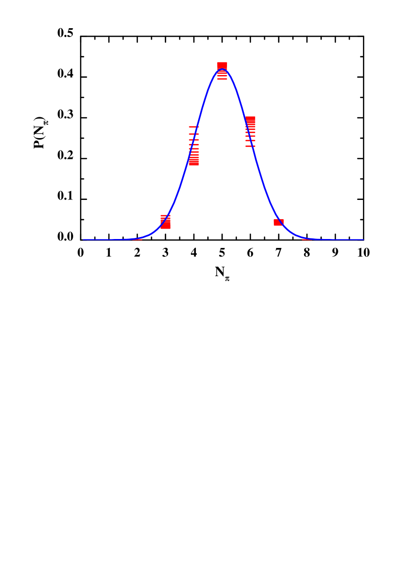
Figure 2: The distribution in the final number of pions $P(N_{\pi})$ for $p\bar{p}$ annihilation at invariant energies 2.3 GeV $\leq\sqrt{s}\leq$ 4 GeV (short lines). The solid line is the gaussian parametrization (25) that is fitted to the experimental data.

excluding 3 vector mesons in the final channel. According to (26) the distribution in the final number of pions (including the explicit vector meson decays to pions) can be evaluated as a function of $\sqrt{s}$ since it only depends on the phase space and the number of possible final states $N_{fin}^{c}$ in each channel $c$. The numerical results are displayed in Fig. 2 for 2.3 GeV $\leq\sqrt{s}\leq$ 4 GeV in comparison to the parametrization (25) (solid line). Here the horizontal bars indicate the range of $N_{\pi}$-pion probabilities when varying $\sqrt{s}$ from 2.3 to 4 GeV. Obviously, the simple phase-space model (26) is in a fair agreement with the experimental observation. For related or more extended models for $p\bar{p}$ annihilation the reader is referred to Ref. [25].

For the backward reactions, i.e. the 3 meson fusion to a $B\bar{B}$ pair, the quarks and antiquarks are redistributed in a baryon and antibaryon, respectively, incorporating the baryons $N,\Delta,\Lambda,\Sigma,\Sigma^{*},\Xi,\Xi^{*},\Omega$ as well as their antiparticles. In line with (26) the relative population of states (with the same quark content) is determined by phase space, i.e.

$$P_{c^{\prime}}(\sqrt{s};M_{1},M_{2})=N_{2}(\sqrt{s})\ R_{2}(\sqrt{s};c^{\prime}=(M_{1},M_{2}))\ (2s_{1}+1)(2s_{2}+1)=$$

$$N_{2}(\sqrt{s})\ R_{2}(\sqrt{s};M_{1},M_{2})\ N_{B}^{c^{\prime}},$$ (29)

where $N_{B}^{c^{\prime}}$ now denotes the number of final states for the particular mass channel $c^{\prime}$ in the backward reaction. The absolute normalization $N_{2}(\sqrt{s})$ is fixed again by the constraint $\sum_{c^{\prime}}P_{c^{\prime}}$ = 1.

As an example consider the reactions $\pi^{-}\pi^{+}\pi^{-}$ or $\pi^{-}\rho^{+}\pi^{-}$ or $\pi^{-}\rho^{+}\rho^{-}$ (and isospin combinations), i.e. $\bar{u}d+\bar{d}u+\bar{u}d\rightarrow(\bar{u}\bar{u}\bar{d})+(udd)$: here the final states may be either $\bar{p}+n$, $\bar{\Delta}^{-}+n$, $\bar{p}+\Delta^{0}$ or $\bar{\Delta}^{-}+\Delta^{0}$ within the Fock space considered. Note, that the final states with a $\Delta$-resonance are favored due to the spin factors in (29), however, somewhat suppressed by the 2-body phase-space integral $R_{2}(\sqrt{s})$ for low $\sqrt{s}$.

One is thus left with the $B\bar{B}$ annihilation problem

$$\frac{dN_{coll}[B\bar{B}\rightarrow 3\ mesons]}{dtdV}=\sum_{c}\sum_{c^{\prime}}\frac{1}{(2\pi)^{6}}\int\frac{d^{3}p_{1}}{2E_{1}}\,\frac{d^{3}p_{2}}{2E_{2}}\ W_{2,3}(\sqrt{s})$$ (30)

$$\times N_{3}(\sqrt{s})\ R_{3}(p_{1}+p_{2};c=(M_{3},M_{4},M_{5}))\ N_{fin}^{c}\ f_{i}(x,p_{1})f_{j}(x,p_{2}),$$

where $(M_{1},M_{2})$ denote the baryon and antibaryon masses in the channel $c^{\prime}$ and $(M_{3},M_{4},M_{5})$ the final meson masses in the channel $c$. Eq. (30) can be rewritten as

$$\frac{dN_{coll}[B\bar{B}\rightarrow 3\ mesons]}{dtdV}=$$ (31)

$$\sum_{c}\sum_{c^{\prime}}\frac{1}{(2\pi)^{6}}\int d^{3}p_{1}\ d^{3}p_{2}\ P^{2,3}_{cc^{\prime}}(\sqrt{s})\ f_{i}(x,p_{1})f_{j}(x,p_{2})$$

with the channel probabilities

$$P^{2,3}_{cc^{\prime}}(\sqrt{s})=\frac{1}{4E_{1}E_{2}}\,W^{2,3}(\sqrt{s})\ N_{3}(\sqrt{s})\ R_{3}(p_{1}+p_{2};(M_{3},M_{4},M_{5}))\ N_{fin}^{c}.$$ (32)

Note, that by construction we have

$$\sum_{c}P^{2,3}_{cc^{\prime}}(\sqrt{s})=\frac{1}{4E_{1}E_{2}}\,W^{2,3}(\sqrt{s})=v_{rel}\ \sigma_{ann}(\sqrt{s})_{c^{\prime}},$$ (33)

where $v_{rel}$ denotes the relative velocity (20) and $\sigma_{ann}(\sqrt{s})_{c^{\prime}}$ is the total annihilation cross section for $B\bar{B}$ pairs of channel $c^{\prime}$.

The backward invariant collision rate is given by

$$\frac{dN_{coll}[3\ mesons\rightarrow B\bar{B}]}{dtdV}=\sum_{c}\sum_{c^{\prime}}\frac{1}{(2\pi)^{9}}\int\left(\prod_{k=3}^{5}\frac{d^{3}p_{k}}{2E_{k}}\right)\ W_{2,3}(\sqrt{s})$$ (34)

$$\times N_{2}(\sqrt{s})\ R_{2}(\sum_{k=3}^{5}p_{k};c^{\prime}=(M_{1},M_{2}))\ N_{B}^{c^{\prime}}\left(\prod_{k=3}^{5}f_{k}(x,p_{k})\right).$$

Using Eq. (17), the relation (19) for 3 mesons in the final state and (33) one arrives at

$$\frac{dN_{coll}[3\ mesons\rightarrow B\bar{B}]}{dtdV}=\sum_{c}\sum_{c^{\prime}}\frac{1}{(2\pi)^{9}}\int\frac{d^{3}p_{3}}{2E_{3}}\,\frac{d^{3}p_{4}}{2E_{4}}\,\frac{d^{3}p_{5}}{2E_{5}}\,4E_{1}E_{2}\$$ (35)

$$\times v_{rel}\ \sigma(\sqrt{s})_{c^{\prime}}\ \frac{N_{2}(\sqrt{s})}{N_{3}(\sqrt{s})}\frac{R_{2}(P^{\mu};c^{\prime}=(M_{1},M_{2}))}{R_{3}(P^{\mu};c=(M_{3},M_{4},M_{5}))}\frac{N_{B}^{c^{\prime}}}{N_{fin}^{c}}$$

$$\hskip 85.35826pt\times f_{3}(x,p_{3})f_{4}(x,p_{4})f_{5}(x,p_{5})$$

for the backward reaction $3+4+5\rightarrow 1+2$. Eq. (35) can now be rewritten as

$$\frac{dN_{coll}[3\ mesons\rightarrow B\bar{B}]}{dtdV}=$$ (36)

$$\sum_{c}\sum_{c^{\prime}}\frac{1}{(2\pi)^{9}}\int d^{3}p_{3}\ d^{3}p_{4}\ d^{3}p_{5}\ P^{3,2}_{cc^{\prime}}(\sqrt{s})\ f_{3}(x,p_{3})f_{4}(x,p_{4})f_{5}(x,p_{5})$$

with the ’transition integrand’

$$P^{3,2}_{cc^{\prime}}(\sqrt{s})=\frac{E_{1}E_{2}}{2E_{3}E_{4}E_{5}}v_{rel}\ \sigma(\sqrt{s})_{c^{\prime}}\ \frac{N_{2}(\sqrt{s})}{N_{3}(\sqrt{s})}\frac{R_{2}(P;c^{\prime}=(M_{1},M_{2}))}{R_{3}(P;c=(M_{3},M_{4},M_{5}))}\ \frac{N_{B}^{c^{\prime}}}{N_{fin}^{c}},$$ (37)

which is of dimension GeV^-3 or fm³.

3 Numerical implementation

For a reformulation of the ’transition integrands’ (specified in (37)) in a test-particle representation one has to recall that the average density of a meson with quantum numbers $k$ is obtained by integration over momentum as:

$$n_{k}(x)=\frac{1}{(2\pi)^{3}}\int d^{3}p\ f_{k}(x,p),$$ (38)

where e.g. charge, strange flavor content, total spin and spin projection are specified by the discrete quantum number $k$. The conversion formula thus reads:

$$\frac{1}{(2\pi)^{3}}\int d^{3}p\ f_{k}(x,p)\rightarrow\frac{1}{dV}\sum_{i\ \epsilon\ dV},$$ (39)

where $dV$ is a (small) finite volume and the sum runs over all test particles in the volume $dV$ with quantum numbers $k$. The number of $B\bar{B}$ annihilations in the volume $dV$ during the time $dt$ is thus given by [62]

$$N_{B\bar{B}}=\frac{dt}{dV}\sum_{i,j\ \epsilon\ dV}v_{rel}(i,j)\sigma_{ann}(\sqrt{s}_{i,j})$$ (40)

with the invariant energy squared

$$s_{i,j}=(p_{1}+p_{2})^{2},$$ (41)

where $p_{1},p_{2}$ denote the 4-momenta of the colliding $B\bar{B}$ pair. The relative velocity $v_{rel}(i,j)$ is given by (20) while the annihilation cross section $\sigma_{ann}(\sqrt{s})$, furthermore, has to be specified for all baryon-antibaryon pairs. This cross section is rather well known for nucleon-antinucleon reactions [25, 64, 63], however, the channels involving $\Lambda,\Sigma,\Sigma^{*},\Xi,\Xi^{*},\Omega^{-}$ baryons or their antiparticles are not available experimentally by now and have to be modeled to some extent.

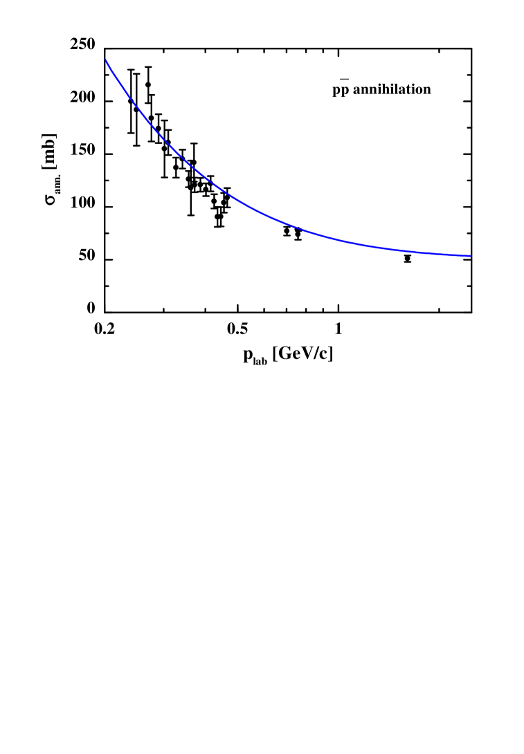
Figure 3: The annihilation cross section $\sigma_{ann.}$ for the $p\bar{p}$ reaction as a function of the laboratory momentum $p_{lab}$ from Ref. [63] in comparison to the approximation (42) (solid line).

For guidance we recall that the product $v_{rel}\ \sigma_{ann}(\sqrt{s})\approx$ 50 mb for a wide range of energies $\sqrt{s}$ in case of $p\bar{p}$ annihilation. This is demonstrated explicitly in Fig. 3, where the experimental annihilation cross section for $p\bar{p}$ from Ref. [63] is compared to the approximation

$$\sigma_{ann}(\sqrt{s})=\frac{50[mb]}{v_{rel}},$$ (42)

which holds well in the dynamical range of interest. We thus can adopt the Boltzmann limit (23) to estimate the $B\bar{B}$ annihilation time at nucleon density $\rho$ as

$$\tau_{ann.}\approx(5fm^{2}\rho)^{-1}\approx 1.2\ \frac{\rho_{0}}{\rho}\ [fm/c].$$ (43)

In this work we will proceed with dynamical calculations in the strangeness sector $S$=0, thus essentially addressing the $\bar{p}$ abundancies in relativistic nucleus-nucleus collisions. In this case the approach formulated above does not involve any new parameter or cross section; it is just an extension of the HSD approach [20, 54, 65] to include the $B\bar{B}\leftrightarrow$ 3 meson reactions by detailed balance.

The number of backward reactions by 3 mesons in the test-particle picture in the volume $dV$ and time $dt$ according to (35) for a given mass channel $c^{\prime}$ is given by

$$N_{3meson}=\frac{dt}{dVdV}\sum_{i,j,k\ \epsilon\ dV}\frac{E_{1}E_{2}}{2E_{i}E_{j}E_{k}}v_{rel}(1,2)\sigma(\sqrt{s})_{c^{\prime}}$$

$$\times\frac{N_{2}(\sqrt{s})}{N_{3}(\sqrt{s})}\frac{R_{2}(\sqrt{s};c^{\prime}=(M_{1},M_{2}))}{R_{3}(\sqrt{s};c=(M_{i},M_{j},M_{k}))}\frac{N_{B}^{c^{\prime}}}{N_{fin}^{c}}=\sum_{i,j,k\ \epsilon\ dV}\ P_{ijk},$$ (44)

where the channel $c$ is defined by the colliding mesons (cf. (24)) and the outgoing channel $c^{\prime}$ by the $B\bar{B}$ pair with masses $M_{1}$ and $M_{2}$ and energies $E_{1}$ and $E_{2}$, respectively. In (44) the summation over the mesons in the volume $dV$ is restricted to $i<j<k$ in case of 3 identical mesons (e.g. 3 pions) and to $i<j$ in case of 2 identical mesons $i,j$ in order to account for the statistical factor $N_{id}!$ in Eq. (27).

Eqs. (40) and (44) are well suited for a Monte Carlo decision problem, i.e. a transition is accepted if the probability $P_{ijk}$ is larger than some random number in the interval [0,1]. One has to assure only, that all $P_{ijk}$ are smaller than 1, which – for a fixed volume $dV$ – can easily be achieved by adjusting the time-step $dt$. This evaluation of scattering probabilities is Lorentz-invariant and does not suffer from geometrical collision criteria as in the standard approaches [66, 67], that imply a different sequence of collisions when changing the reference frame by a Lorentz transformation [68]. For $2\leftrightarrow 2$ transitions it has first been employed and tested by Lang et al. in Ref. [62]; this method is also implemented in the HSD approach, where it can be used optionally instead of the standard geometrical collision criteria as described e.g. in Refs. [57, 66, 69]. The present implementation in this respect is a straight forward generalization of the concept in Ref. [62] to $2\leftrightarrow 3$ reactions. It is worth to point out that this numerical implementation is a promising way to treat $n\leftrightarrow m$ transitions in transport theories without violating covariance or causality. In case of infinitesimal volumes $dV$ and time steps $dt$ it gives the correct solution to the many-particle Boltzmann equation.

For the actual numerical calculations a dynamical time-step size $dt$ is employed which on average amounts to $dt\approx 0.5/\gamma_{cm}$ [fm/c], where $\gamma_{cm}$ is the Lorentz factor in the nucleus-nucleus cms, i.e. $\gamma_{cm}\approx$ 9.3 for collisions of $Pb+Pb$ at 160 A$\cdot$GeV. The volume $dV$ is chosen to be $dV=A\ dz$ with the transverse area $A=9fm^{2}$ and $dz=3/\gamma_{cm}$ [fm]. Variations of these parameters within a factor of 3 do not change the numerical results to be presented below. In order to avoid numerical artefacts, that are due to the finite volume $dV$, a $B\bar{B}$ pair, that has been produced by meson fusion, is not allowed to annihilate on each other again without performing an additional collision in between. On the other hand, the mesons stemming from a particular $B\bar{B}$ annihilation are not allowed to fuse again with the same partners for the backward reaction, if no intermediate extra collision has occured.

As a numerical test the number of collisions in a single box of volume 10 fm³ during the time $dt$ =1 fm/c has been calculated with spatially uniform phase-space distributions given by a classical system of hadrons in thermal and chemical equilibrium, i.e.

$$f_{k}(p)=\frac{(2s+1)(2I+1)}{(2\pi)^{3}}{\exp(-E_{k}(p)/T)}$$ (45)

with $s$ and $I$ denoting spin and isospin, respectively. The particles taken into account are $N,\Delta$ and their antiparticles and $\pi,\rho,\omega$ on the meson side in the strangeness sector $S$=0. The numerical results for the number of $B\bar{B}$ annihilation collisions ($\rightarrow\pi\rho\rho$) are shown in Fig. 4 in terms of the dashed line as a function of $\sqrt{s}$, which corresponds to the invariant energy in an individual collision. As can be seen from Fig. 4 the dashed line very well coincides with the solid line that corresponds to the energy differential number of $\pi\rho\rho$ collisions for the backward reactions. Thus the numerical scheme employed well reproduces the detailed balance relation in thermal equilibrium for a given channel combination $cc^{\prime}$. Without explicit representation we mention that the detailed balance relation is fulfilled for all channel combinations $cc^{\prime}$ specified above.

4 Nucleus-nucleus collisions

4.1 SPS energies

The most complete set of data on antibaryon production in nucleus-nucleus collisions is available from the NA44 [72], NA49 [30] and WA97 [31, 32] Collaborations for $Pb+Pb$ collisions at SPS energies of 160 A$\cdot$GeV, that allow for stringent tests of the dynamics proposed. Since the extension of the HSD transport approach is described in the previous Section and no new parameters enter into the calculations, we proceed with the actual results.

4.1.1 Cascade calculations

Though antiproton self energies have been found to be important in nucleus-nucleus collisions at subthreshold energies [19, 20, 21], we start with cascade calculations because the initial invariant energy per nucleon is large compared to the $B\bar{B}$ threshold. However, before coming to the antibaryon abundancies the performance of the HSD transport approach has to be tested in comparison to experimental data for baryons and mesons. Since detailed differential spectra for protons, hyperons, pions and kaons have been presented in Ref. [65] in comparison to the experimental data for central collisions of $Pb+Pb$ at 160 A$\cdot$GeV, we concentrate here on particle abundancies as a function of ’centrality’. The latter is defined by the number of participants $A_{part}$, which is extracted from the transport calculation at impact parameter $b$ as

$$A_{part}(b)=2A-N_{0}(b),$$ (46)

where $N_{0}(b)$ is the number of nucleons that were not involved in any hard scattering process.

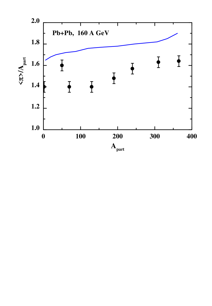
Figure 5: The calculated average number of charged pions $<\pi>$ divided by $A_{part}$ as a function of centrality for $Pb+Pb$ at 160 A$\cdot$GeV in comparison to the data from Ref. [30].

The average number of charged pions $<\pi>=(<\pi^{+}+\pi^{-}>)/2$ (divided by $A_{part}$) is shown in Fig. 5 as a function of $A_{part}$ in comparison to the data from Ref. [30] for $Pb+Pb$ at 160 A$\cdot$GeV. The number of pions per participant nucleon is found to be approximately constant within 10 % as a function of centrality; there is a slight trend in the data as well as in the HSD calculations (solid line) for an increase of $<\pi>/A_{part}$ for central collisions. However, the HSD transport calculations overestimate the pion abundancy by about 20 %. Such an overprediction of pion multiplicities in heavy systems occurs in other transport approaches as well [53, 70] – or is even higher – and is not well understood so far. At SIS energies of 1–2 A$\cdot$GeV it has been argued in Ref. [71] that a quenching of nucleon resonances at baryon densities $\rho\geq\rho_{0}$ might be responsible for the relative pion suppression seen experimentally in heavy systems, but it is not yet clear if such a mechanism will also explain the discrepancies at SPS energies. We thus have to keep in mind this overprediction of pions especially when comparing particle ratios (see below).

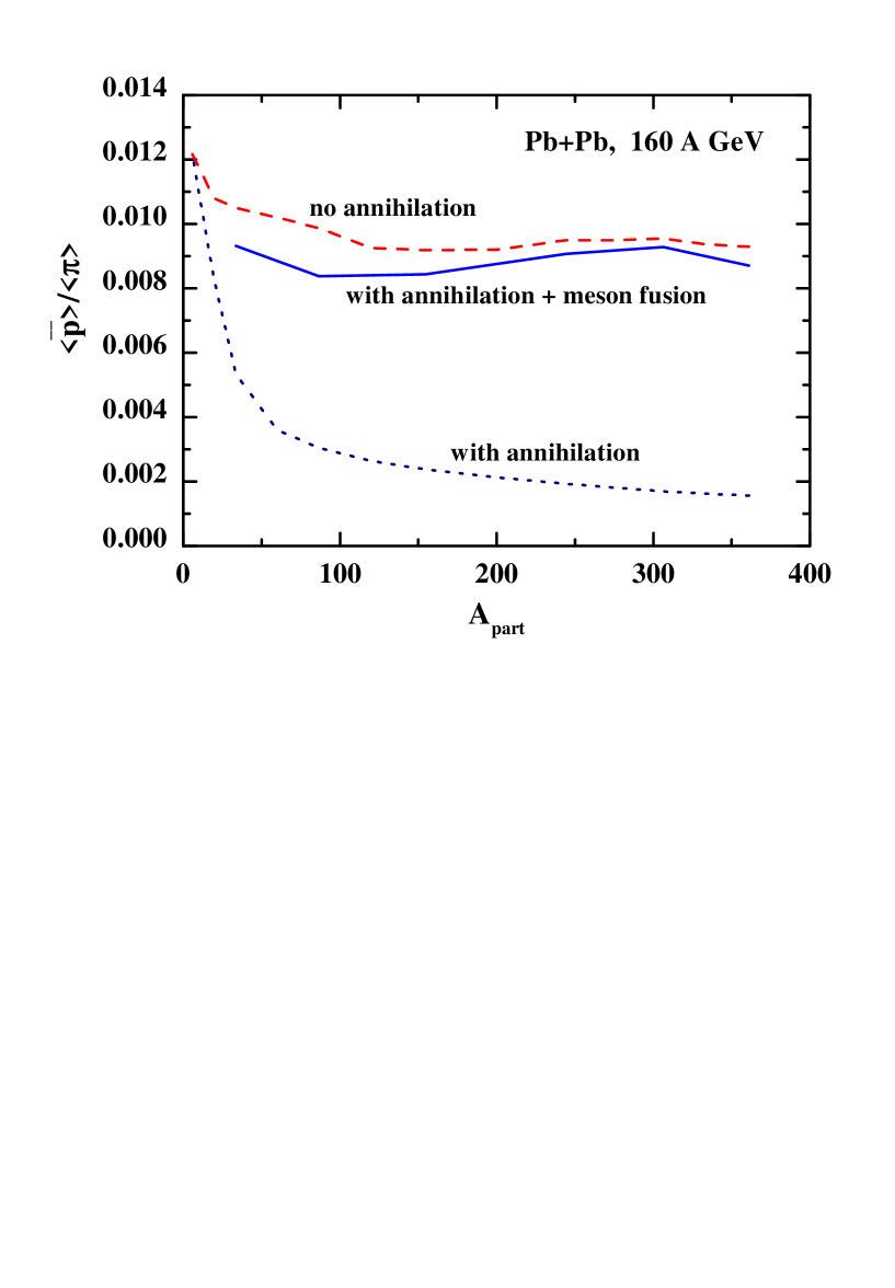
Figure 6: The ratio of antiprotons to the average number of charged pions $<\pi>$ as a function of centrality for $Pb+Pb$ at 160 A$\cdot$GeV within different approximations. The dashed line reflects calculations without annihilation of antibaryons, the dotted line includes the annihilation channels while the solid line stands for the calculations with both, the annihilation and meson fusion channels.

The effect of antibaryon annihilation and reformation by means of meson fusion channels is shown in Fig. 6, where the $<\bar{p}>/<\pi>$ ratio is displayed for $Pb+Pb$ at 160 A$\cdot$GeV as a function of $A_{part}$. The dashed line shows a calculation without including annihilation channels in the transport calculation, the dotted line gives the results including the annihilation to mesons while the solid line is obtained when including both, annihilation and meson fusion channels by detailed balance. The first point in Fig. 6 gives the numerical result for $NN$ interactions at $T_{lab}$ = 160 GeV ($A_{part}$ = 2). As shown in Table 1 of Ref. [65], the description of the HSD approach for $pp$ interactions is well in line with the data on $\pi^{+},\pi^{0},\pi^{-},K^{+},K^{-},K^{0}_{s}$, $\Lambda+\Sigma^{0}$, $\bar{\Lambda}+\bar{\Sigma}^{0}$ as well as $p$ and $\bar{p}$ multiplicities at SPS energies, such that this point may serve for reference to the particle abundancies in the elementary $NN$ interaction. As seen from Fig. 6 the $<\bar{p}>/<\pi>$ ratio slightly drops with centrality for peripheral reactions, however, stays approximately constant for $A_{part}\geq$ 150 when neglecting annihilation. Thus antiprotons in central $Pb+Pb$ collisions are produced less frequent than pions by about 30 % relative to the $NN$ interaction in vacuum. The effect of annihilation (dotted line) sets in already for peripheral reactions and amounts to a factor $\sim$6–7 suppression for central collisions. The latter suppression is sensitive to the formation time $\tau_{F}$ of the antibaryons and becomes larger (smaller) for shorter (longer) $\tau_{F}$. In the actual calculations we have used $\tau_{F}$ = 0.8 fm/c for all hadrons [65]. When including annihilation as well as meson fusion channels by detailed balance, the $<\bar{p}>/<\pi>$ ratio (solid line) becomes again close to the calculation that does not include annihilation nor meson fusion reactions to $B\bar{B}$ (dashed line). Thus on average the annihilation channels are almost compensated by the reproduction channels.

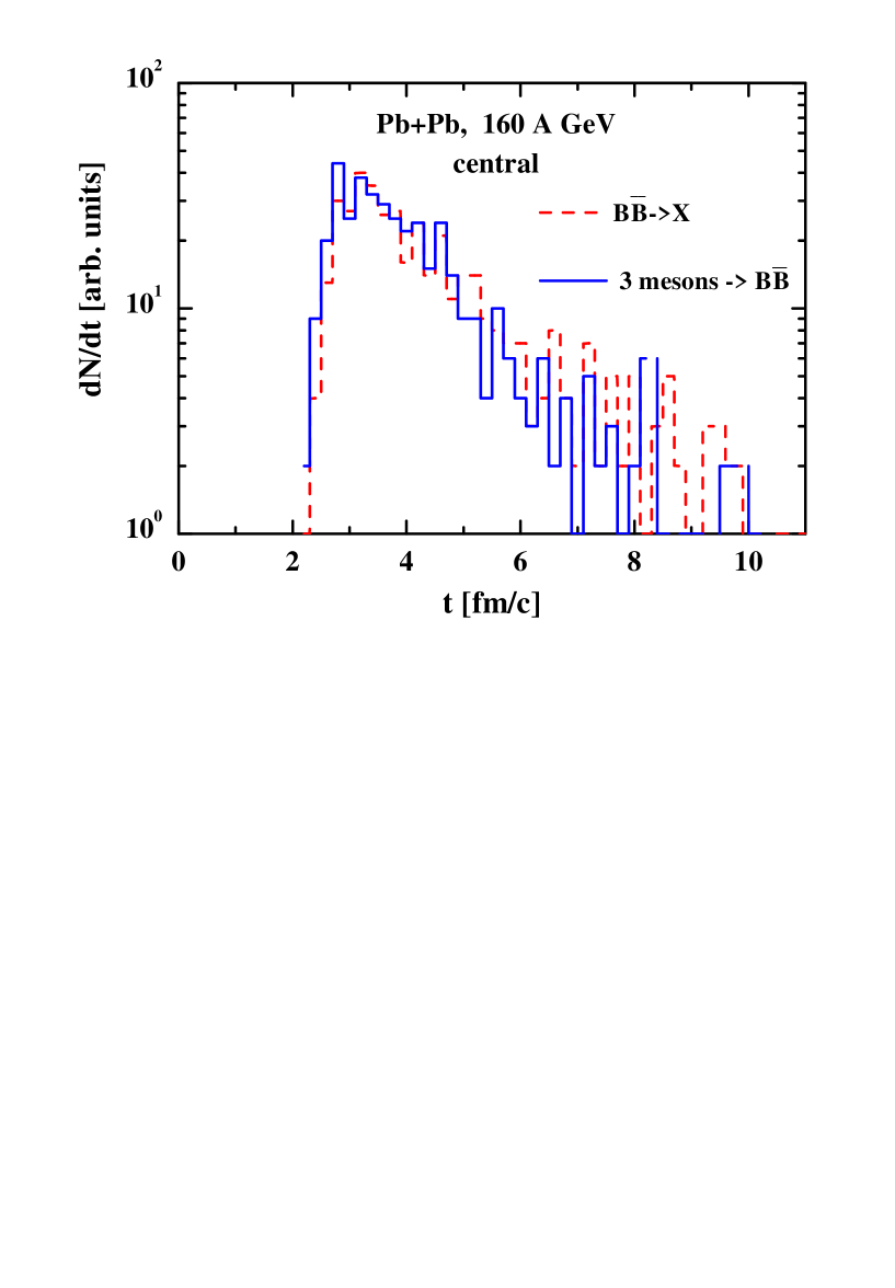
Figure 7: The annihilation rate $B\bar{B}\rightarrow 3mesons$ (dashed histogram) for a central $Pb+Pb$ collision at 160 A$\cdot$GeV as a function of time in comparison to the backward reaction rate (solid histogram) within the HSD transport approach.

In order to get some idea about the dynamical origin of the approximately constant $\bar{p}/\pi$ ratio shown in Fig. 6 by the solid line the reaction rate $B+\bar{B}\rightarrow mesons$ (dashed histogram in Fig. 7 ) is compared to the backward reaction rate (solid histogram in Fig. 7) for a central collision of $Pb+Pb$ at 160 A$\cdot$GeV. Fig. 7 demonstrates that both rates are comparable within the statistics. Thus an approximate local chemical equilibrium is established very fast between the nonstrange antibaryon degrees of freedom and the nonstrange mesons $\pi,\rho$ and $\omega$. The latter fact is supported by the absolute number of reactions $B\bar{B}\rightarrow mesons$ which is about 4-5 times higher than the final number of antibaryons per event. On the other hand, the number of backward reactions is $\sim$ 96% of the number of annihilation reactions leading to a small net absorption of the antibaryons produced initially by baryon-baryon ($\sim$ 73%) or meson-baryon ($\sim$ 27%) inelastic collisions. Only $\sim 12$% of the final antibaryons stem from ’hard’ baryon-baryon or meson-baryon reactions; the dominant amount of final $\bar{p}$’s ($\sim$ 88%) are from the 3 meson fusion reactions indicating that the memory with respect to the initial ’hard’ collision phase is practically lost.

One might worry about the sensitivity of these results to the annihilation cross section $\sigma_{ann}(\sqrt{s})$ that so far has been taken to be the free cross section (in the parametrization from Ref. [19]). However, this quantity might change in the medium due to screening effects. It is clear that any enhancement of this cross section will lead to an even faster equilibration in the light flavor degrees of freedom and to a more perfect chemical equlibrium. Thus numerical calculations have been performed for central $Pb+Pb$ collisions at 160 A$\cdot$GeV by assuming that $\sigma_{ann}$ is reduced by a factor of 2. This leads to a reduction of the total number of annihilation reactions (and backward reactions) by a factor of 2 – which essentially reduces the numerical statistics – but leaves the conclusions unchanged. Thus the findings from Figs. 6 and 7 are robust against ’reasonable’ modifications of the in-medium transition rates.

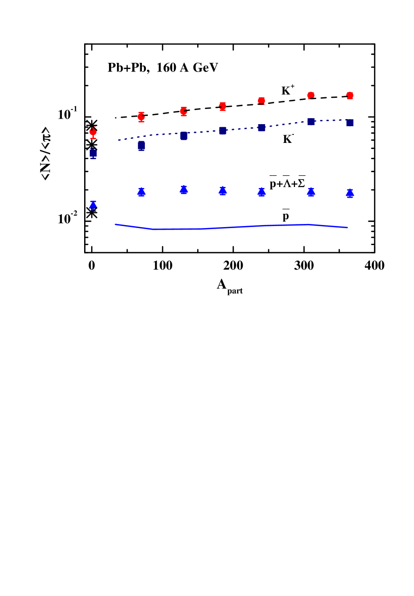
Figure 8: The calculated $K^{+}/\pi$ (dashed), $K^{-}/\pi$ (dotted) and $\bar{p}/\pi$ (solid) ratio for $Pb+Pb$ at 160 A$\cdot$GeV as a function of the number of participating nucleons $A_{part}$. The experimental data are taken from Ref. [30]; the latter data for antiprotons include also the feeddown from $\bar{\Lambda}$ and $\bar{\Sigma}^{0}$, respectively. The stars for $A_{part}$ = 2 denote the transport results for $K^{+}/\pi$, $K^{-}/\pi$ and $\bar{p}/\pi$ ratios in case of $NN$ reactions at $T_{lab}$ = 160 GeV.

The numerical abundancies for $K^{\pm}$ mesons and antiprotons relative to the average charged pion multiplicity $<\pi>=<\pi^{+}+\pi^{-}>/2$ are displayed in Fig. 8 for $Pb+Pb$ at 160 A$\cdot$GeV as a function of $A_{part}$. The comparison of the calculations with the data from Ref. [30] indicates that the dependence of the $K^{\pm}$ multiplicities on $A_{part}$ is roughly met – except a single point for $K^{-}$ at rather peripheral reactions – in line with the earlier analysis in Refs. [20, 65], which concentrated on central collisions in this system. However, the $\bar{p}/\pi$ ratio is lower by about a factor of 2 compared to the data of the NA49 Collaboration that also include the feeddown from $\bar{\Lambda}$ and $\bar{\Sigma}^{0}$ due to the weak interaction. Since the latter contribution is presently unknown one might either speculate that the $\bar{\Lambda}+\bar{\Sigma}^{0}$ abundancy is comparable to the antiproton abundancy or that antiproton self energy effects might be responsible for the experimental observation.

4.1.2 Antiproton self energies

As shown in Refs. [16, 19, 20, 21] the production of antiprotons at SIS energies of 1.4–2.1 A$\cdot$GeV as well as in $p+A$ reactions is described by adopting attractive self energies for the antiprotons in the range of -100 to -150 MeV at normal nuclear matter density $\rho_{0}$. Especially in $p+A$ reactions the backward production channels by a couple of mesons are statistically irrelevant as can be easily checked by the transport model described above. The question thus arises if such ’established’ antiproton self energies for densities 1–3 $\rho_{0}$ might also be responsible for an enhancement of the $\bar{p}$ yield at SPS energies in the $Pb+Pb$ system.

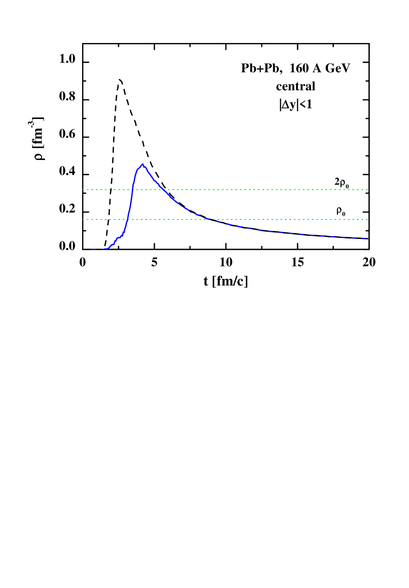
Figure 9: The baryon density in a central expanding cylinder (see text) for $|\Delta y|_{cm}\leq$ 1 in case of a central collision of $Pb+Pb$ at 160 A$\cdot$GeV in the HSD approach as a function of time. The solid line shows the density of ’formed’ baryonic states while the dashed line stands for the net quark density $\rho_{q}/3$, while merges with the baryon density in the expansion phase. The dotted lines at $\rho_{0}$ and $2\rho_{0}$ are drawn to guide the eye.

To examine this possibility we show in Fig. 9 the time evolution of the baryon-density in a central cylinder of transverse radius $R_{T}$ = 5 fm, that has moving boundaries with the expanding hadronic system in longitudinal direction. The solid line denotes the average density of ’formed’ baryonic states whereas the dashed line represents the net quark density $\rho_{q}/3$ which merges with the baryon density in the later expansion phase. Both densities have been evaluated in the cms rapidity interval $|\Delta y|_{cm}\leq$ 1 in order to exclude spectator nucleons and to gate on midrapidity physics. The difference between the solid and dashed line in Fig. 9 has to be attributed to ’non-hadronic’ states, which in the HSD approach are quarks and diquarks (as well as their antiparticles) that constitute the ends of ’strings’ or continuum excitations of the hadrons. As can be seen from Fig. 9 the ’non-hadronic’ phase lasts about 2.2 fm/c which is roughly the diameter of the target ($2R$) divided by the Lorentz-factor $\gamma_{cm}\approx$ 9.3 plus the hadron formation time $\tau_{F}$ = 0.8 fm/c [20],

$$\tau_{nonhad.}\approx\frac{2R}{\gamma_{cm}}+\tau_{F}.$$ (47)

Then a mixed phase of ’partons’ and ’formed’ hadrons comes up which practically ends around 6 fm/c where all continuum excitations have merged to hadrons or hadronic resonant states. Quite remarkably, the density of ’formed’ baryons is about $2\rho_{0}$ at the beginning of the pure hadronic expansion phase. Now the $B\bar{B}$ annihilation rate (in Fig. 7) starts with a maximum around 3 fm/c – when the ’baryons’ also start to hadronize – along with the meson fusion reactions that last up to about 8 fm/c. The characteristic time scale for the decrease of the annihilation/fusion rate is $\tau_{prod}\approx$1.6 fm/c for central $Pb+Pb$ reactions at the SPS as extracted from Fig. 7 using an exponential ansatz. During the $B\bar{B}$ production phase by meson fusion from 3–8 fm/c the density of baryons drops from $\sim 2.5\rho_{0}$ to $\rho_{0}$. Employing (43) the time scale for annihilation at these densities changes from 0.5 – 1.2 fm/c, which is considerably shorter than the characteristic production time scale of 1.6 fm/c. The approximate chemical equilibration between mesons and antibaryons thus is no surprise according to these simple ’classical’ estimates. On the other hand, the densities of 2.5 $\rho_{0}$ – $\rho_{0}$ are very similar to the densities probed in heavy-ion reactions at SIS energies from 1–2 A$\cdot$GeV [21, 57].

In order to investigate if $\bar{p}$ self energies might be responsible for the experimental antiproton yield, a scalar attractive $\bar{p}$ potential of the form

$$U_{\bar{p}}(\rho)=-\alpha\frac{\rho}{\rho_{0}}$$ (48)

is assumed with $\alpha$ = 100 MeV, where $\rho$ denotes the density of ’formed’ baryons. This amounts to produce and propagate antiprotons with a density-dependent mass $M^{*}=M_{0}+U(\rho)$. For more technical details the reader is referred to Refs. [16, 19]. Note, that when introducing self energies for particles by averaging the latter over many events one no longer performs microcanonical simulations since the field energy is shared between different events. However, quark flavor conservation still holds exactly in each event such that the physical system corresponds to a canonical ensemble.

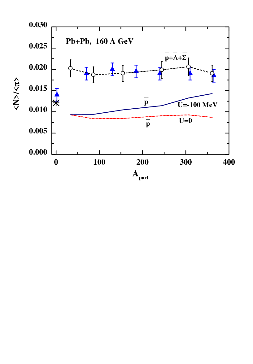
Figure 10: The antiproton to charged pion ratio (see text) as a function of the number of participating nucleons $A_{part}$ for $Pb+Pb$ at 160 A$\cdot$GeV. The dotted line denoted by $U=0$ corresponds to the cascade result (cf. Fig. 8) while the solid line denoted by $U=-100$ MeV corresponds to a calculation with the attractive scalar antiproton potential (48) of -100 MeV at baryon density $\rho_{0}$. The full triangles represent the data from Ref. [30] while the open circles correspond to a cascade calculation including the feeddown from antihyperons according to Eq. (51). The errorbars are due to the limited statistics in the transport calculation. The star for $A_{part}$ = 2 denotes $\bar{p}/\pi$ ratio for $NN$ collisions at $T_{lab}$ = 160 GeV.

The numerical results for the $\bar{p}/<\pi>$ ratio in $Pb+Pb$ collisions at 160 A$\cdot$GeV are displayed in Fig. 10 by the solid line in comparison to the cascade calculation (dashed line) and the experimental data from NA49 [30] (full triangles). It is seen that with increasing centrality or $A_{part}$ there is a slight enhancement of the $\bar{p}$ yield for the potential (48), which vanishes for very peripheral reactions where the average baryon density is very small. The experimental data, however, are still underestimated significantly. This also holds true when accounting for the 20% overprediction of pions in the transport approach (cf. Fig. 5).

4.1.3 Extrapolation for antihyperon production

In view of the approximate chemical equilibrium achieved for the $u,d$ quark sector between mesons and antibaryons – even for reduced annihilation cross sections – one may proceed with speculations on the strangeness ($s\bar{s}$-quark) sector, where no experimental data on the annihilation cross sections are available. However, in case of similar transition matrix elements squared ($\approx$ 5 fm²) the $Y\bar{N}$ and $\bar{Y}N$ channels, where $Y$ stands for the hyperons ($\Lambda,\Sigma,\Sigma^{*}$), will achieve chemical equilibrium with the 3 meson system as before, however, with a $\pi$ or $\rho,\omega$ exchanged by a $K$ or $K^{*},\phi$, respectively (cf. Ref. [51] for the case of 5 meson reaction channels). A further step then consists in replacing another pion or $\rho,\omega$ by a $K$ or $K^{*},\phi$ which will bring the $\Xi,\Xi^{*}$ and $\bar{\Xi},\bar{\Xi}^{*}$ in chemical equilibrium with the $SU(3)_{flavor}$ meson system. Moreover, in case of flavor rearrangement reactions with 3 strange mesons $K,K^{*},\phi$ (or any combinations of those) the $\Omega,\bar{\Omega}$ system might also achieve chemical equilibrium. This will imply for the antibaryon to baryon ratios:

$$\frac{\bar{p}}{p}\approx\frac{K^{-}}{K^{+}}\ \frac{\bar{\Lambda}}{\Lambda}\approx\left(\frac{K^{-}}{K^{+}}\right)^{2}\ \frac{\bar{\Xi}}{\Xi}\approx\left(\frac{K^{-}}{K^{+}}\right)^{3}\ \frac{\bar{\Omega}}{\Omega}.$$ (49)

The relations (49) are easily obtained for a grand canonical ensemble at ’high’ temperature $T$ where Fermi and Bose distributions coincide with the Boltzmann distribution. In this limit the ratios of particles to antiparticles (apart from the temperature $T$) only depend on the chemical potential $\mu_{q}$ for light quarks and $\mu_{s}$ for strange quarks, i.e.

$$\frac{\bar{p}}{p}=\frac{\exp(-(E_{\bar{p}}+3\mu_{q})/T)}{\exp-(E_{p}-3\mu_{q})/T)}=\exp(-6\mu_{q}/T),$$

$$\frac{\bar{K}}{K}=\frac{\exp(-(E_{\bar{K}}-\mu_{s}+\mu_{q})/T)}{\exp(-(E_{K}+\mu_{s}-\mu_{q})/T)}=\exp(2(\mu_{s}-\mu_{q})/T),\$$

$$\frac{\bar{\Lambda}}{\Lambda}=\frac{\exp(-(E_{\bar{\Lambda}}+\mu_{s}+2\mu_{q})/T)}{\exp(-(E_{\Lambda}-\mu_{s}-2\mu_{q})/T)}=\exp(-(2\mu_{s}+4\mu_{q})/T)\$$

$$\frac{\bar{\Xi}}{\Xi}=\frac{\exp(-(E_{\bar{\Xi}}+2\mu_{s}+\mu_{q})/T)}{\exp(-(E_{\Xi}-2\mu_{s}-\mu_{q})/T)}=\exp(-(4\mu_{s}+2\mu_{q})/T)\$$

$$\frac{\bar{\Omega}}{\Omega}=\frac{\exp(-(E_{\bar{\Omega}}+3\mu_{s})/T)}{\exp(-(E_{\Omega}-3\mu_{s})/T)}=\exp(-6\mu_{s}/T),\$$ (50)

where $E_{X},E_{\bar{X}}$ denote the energies of particles and antiparticles, respectively, that are the same when neglecting self energies. Note, that the relations (49) also result from the quark condensation model in Refs. [73, 74], however, involve a slightly different physical picture. In the latter approach the mesons, baryons and antibaryons emerge from an equilibrium QGP state by condensation under the constraint of quark flavor conservation. In the microcanonical transport approach discussed here, the relations (49) come about due to the strong annihilation of antibaryons with baryons and the backward flavor rearrangement channels by detailed balance, i.e. by purely hadronic reaction channels in the expansion phase of the system.

It should be pointed out, that the canonical statistical approach of Ref. [48] – involving an additional parameter of dimension fm³ – well describes the strange and multi-strange baryon and antibaryon abundancies in $Pb+Pb$ collisions at SPS energies. Thus the concept of chemical equilibrium also on the strangeness sector $S$= $\pm 1,\pm 2,\pm 3$ appears compatible with the experimental observations. However, it is argued here that the relations (49) are a consequence of the strong flavor rearrangement reactions between formed hadrons and do not signal the presence of a QGP state.

Assuming chemical equilibrium also for baryons and antibaryons with strangeness then (by Eq. (49)) the $\bar{\Lambda}$ multiplicity is related to the antiproton multiplicity as

$$\bar{\Lambda}\approx\left(\frac{K^{+}}{K^{-}}\times\frac{\Lambda}{p}\right)\ \bar{p}.$$ (51)

All quantities on the r.h.s. of (51) are known from the transport calculation, however, only the interacting number of protons have to be counted in this case since proton spectators have to be excluded in this balance. A rather save way is to take into account only particles at midrapidity for $|\Delta y|\leq$ 1, which then excludes spectator baryons. Thus counting only particles at midrapidity for the ratio in the brackets in (51) the $\bar{\Lambda}$ abundancy is entirely determined by particle ratios that have sufficient statistics in the transport calculation. The resulting $(\bar{p}+\bar{Y})/<\pi>$ ratio for $Pb+Pb$ at 160 A$\cdot$GeV is shown in Fig. 10 by the open circles with error bars that are due to particle statistics in the transport calculation. In this case the experimental multiplicity is reproduced rather well from peripheral to central collisions (within the error bars) suggesting the ratio $\bar{\Lambda}/\bar{p}\approx$ 1 for a wide range of impact parameters. However, a precise experimental separation of antiprotons from antihyperons will be necessary to clarify the present ambiguities.

4.2 AGS energies

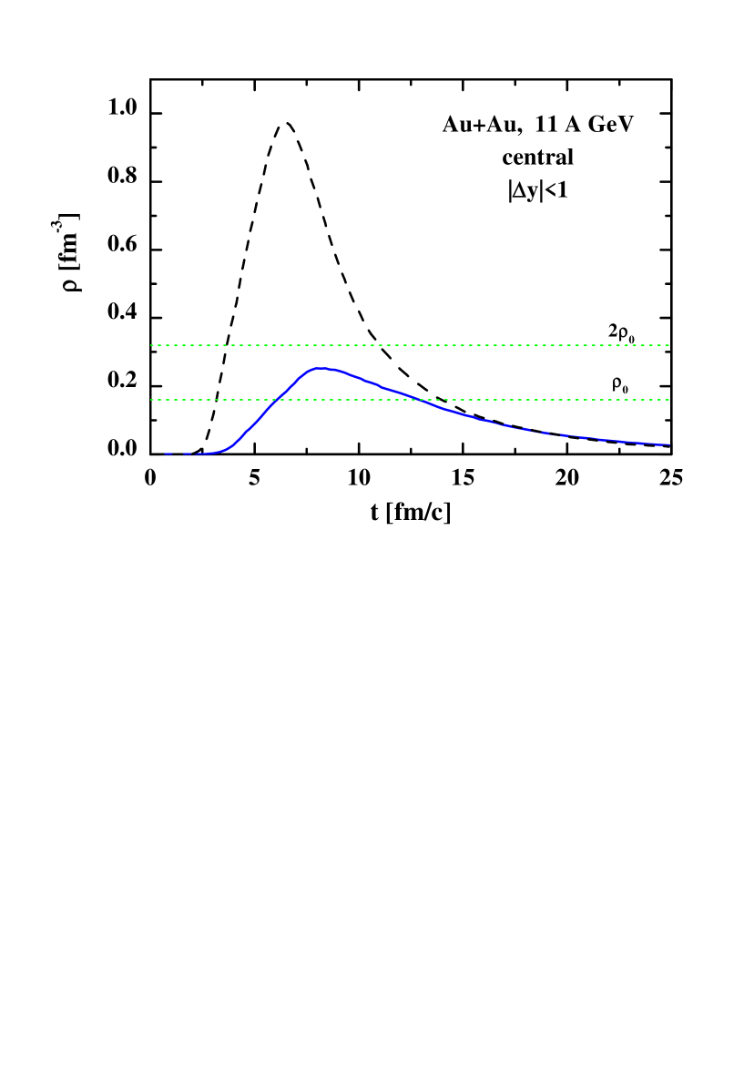
Figure 11: The baryon density in a central expanding cylinder (see text) for $|\Delta y|_{cm}\leq$ 1 in case of a central collision of $Au+Au$ at 11.6 A$\cdot$GeV/c in the HSD approach as a function of time. The solid line shows the density of ’formed’ baryonic states while the dashed line stands for the net quark density $\rho_{q}/3$, while merges with the baryon density in the expansion phase.

The experimental information on antibaryon production at AGS energies is rather scarce and limited to specific rapidity intervals. Since antibaryon yields are also reduced substantially as compared to SPS energies this imposes severe constraints on the statistics in nonperturbative transport calculations. Thus, before addressing any comparison to experimental data, we show in Fig. 11 the density of ’formed’ baryons in a central expanding cylinder of transverse radius $R_{T}$ = 5 fm for $Au+Au$ at 11 A$\cdot$GeV in comparison to the net quark density $\rho_{q}/3$ (dashed line). When comparing to Fig. 9 for $Pb+Pb$ at 160 A$\cdot$GeV roughly the same maximum net quark density is found for $|\Delta y|\leq$ 1, however, the nonhadronic phase characterized by (47), i.e. $\tau_{nonhad.}\approx 6.2$ fm/c, lasts much longer due to the lower Lorentz $\gamma$-factor $\gamma_{cm}\approx 2.6$. Furthermore, the density of ’formed’ baryons is lower than at SPS energies since most of these hadronic states rescatter again on baryons in the medium since the formation time $\tau_{F}$ = 0.8 fm/c is small compared to the reaction time roughly given by $2R/\gamma_{cm}$, where $R$ denotes the radius of the $Au$ nucleus. Thus ’formed’ baryons are reexcited to strings for a couple times during the nucleus-nucleus collision. This phenomenon has been addressed as ’string matter’ in Ref. [75] and should not be interpreted as a state of quark-gluon plasma (QGP).

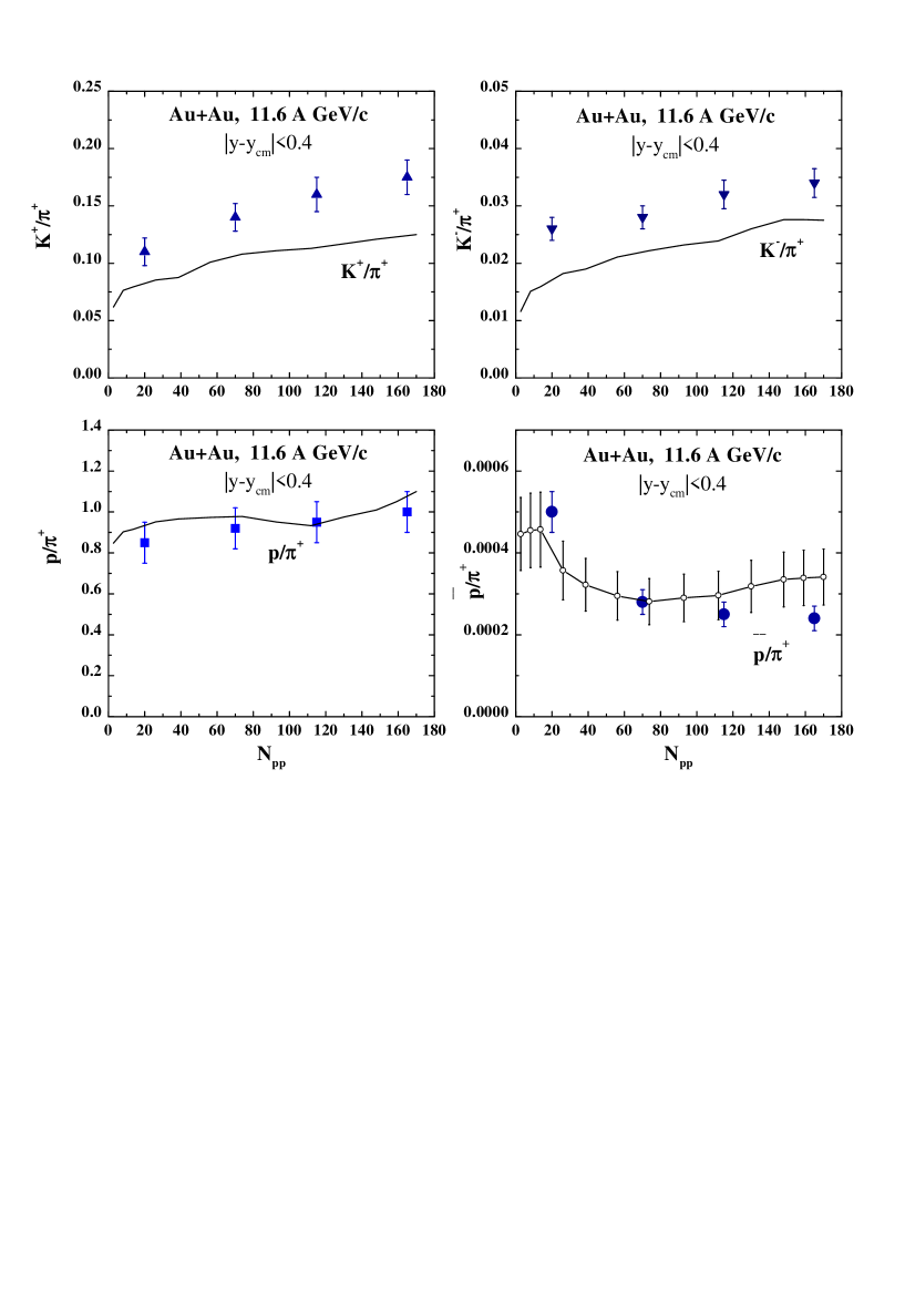
Figure 12: The $K^{+}/\pi^{+}$, $K^{-}/\pi^{+}$, $p/\pi^{+}$ and $\bar{p}/\pi^{+}$ ratio at midrapidity for $Au+Au$ at 11.6 A$\cdot$GeV/c as a function of the number of participating protons $N_{pp}$. The solid line correspond to the HSD transport calculation in the cascade mode for mesons and antibaryons (open circles) while the experimental data (full symbols) are taken from [26].

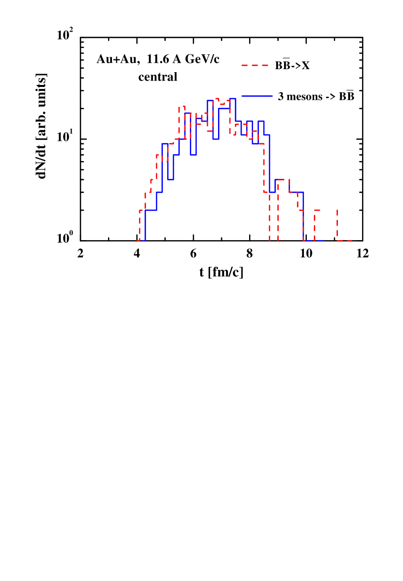
Figure 13: The annihilation rate $B\bar{B}\rightarrow 3mesons$ (dashed histogram) for a central $Au+Au$ collision at 11.6 A$\cdot$GeV/c as a function of time in comparison to the backward reaction rate (solid histogram) within the HSD transport approach.

A comparison of the HSD transport calculations with the experimental data of the E866 Collaboration at midrapidity [26] is presented in Fig. 12 as a function of the participating protons $N_{pp}$ for $Au+Au$ at 11.6 A$\cdot$GeV/c. Whereas the proton to $\pi^{+}$ ratio is rather well described as a function of centrality (lower left part) the $K^{+}/\pi^{+}$ and $K^{-}/\pi^{+}$ ratios are underestimated systematically for all centralities when discarding self energies for the strange hadrons (cf. Refs. [20, 65, 76]). The calculated $K^{+}/K^{-}$ ratio from the HSD calculation is 5$\pm 0.3$ for all centralities rather well in line with the experimental observation at midrapidity. Since strangeness conservation is exactly fulfilled in the calculations this demonstrates that the net production of $s\bar{s}$ quarks by ’hard’ baryon-baryon, baryon-meson and meson-meson reactions is underestimated in the transport approach as discussed in more detail in Refs. [20, 65]. On the other hand the antiproton to $\pi^{+}$ ratio (lower right part) is compatible with the experimental ratios within the error bars indicating an approximately constant value of $\sim 2.5-3\times 10^{-4}$. This roughly constant $\bar{p}/\pi^{+}$ ratio is a consequence of an approximate chemical equilibration as demonstrated in Fig. 13 for a central collision of $Au+Au$ at 11.6 A$\cdot$GeV/c. Here the solid histogram corresponds to the annihilation rate of antibaryons whereas the dashed histogram stands for the backward 3 meson fuse rate. Though the statistics are very limited in this case a net absorption of antibaryons, i.e. the difference in the time integrals of the annihilation rate and 3 meson production rate, is still present in the calculations which amounts to about 20% for central reactions and about 30% for very peripheral reactions of the total number of antibaryons produced in baryon-baryon or meson-baryon reactions. This relative net absorption, however, can only be extracted from transport calculations and is not a measurable quantity experimentally.

The E877 Collaboration, furthermore, has observed a sizeable anti-flow of $\bar{p}$’s in $Au+Au$ reactions at 11.6 A$\cdot$GeV/c [27] which either indicates a strong absorption of antiprotons on baryons or the current of comoving mesons, that fuse to $B\bar{B}$ pairs, and are anticorrelated to the proton current themselves. The present transport calculations reproduce these correlations, however, suffer from large statistical error bars (similar in size to those of the data) such that an explicit comparison is discarded in this work.

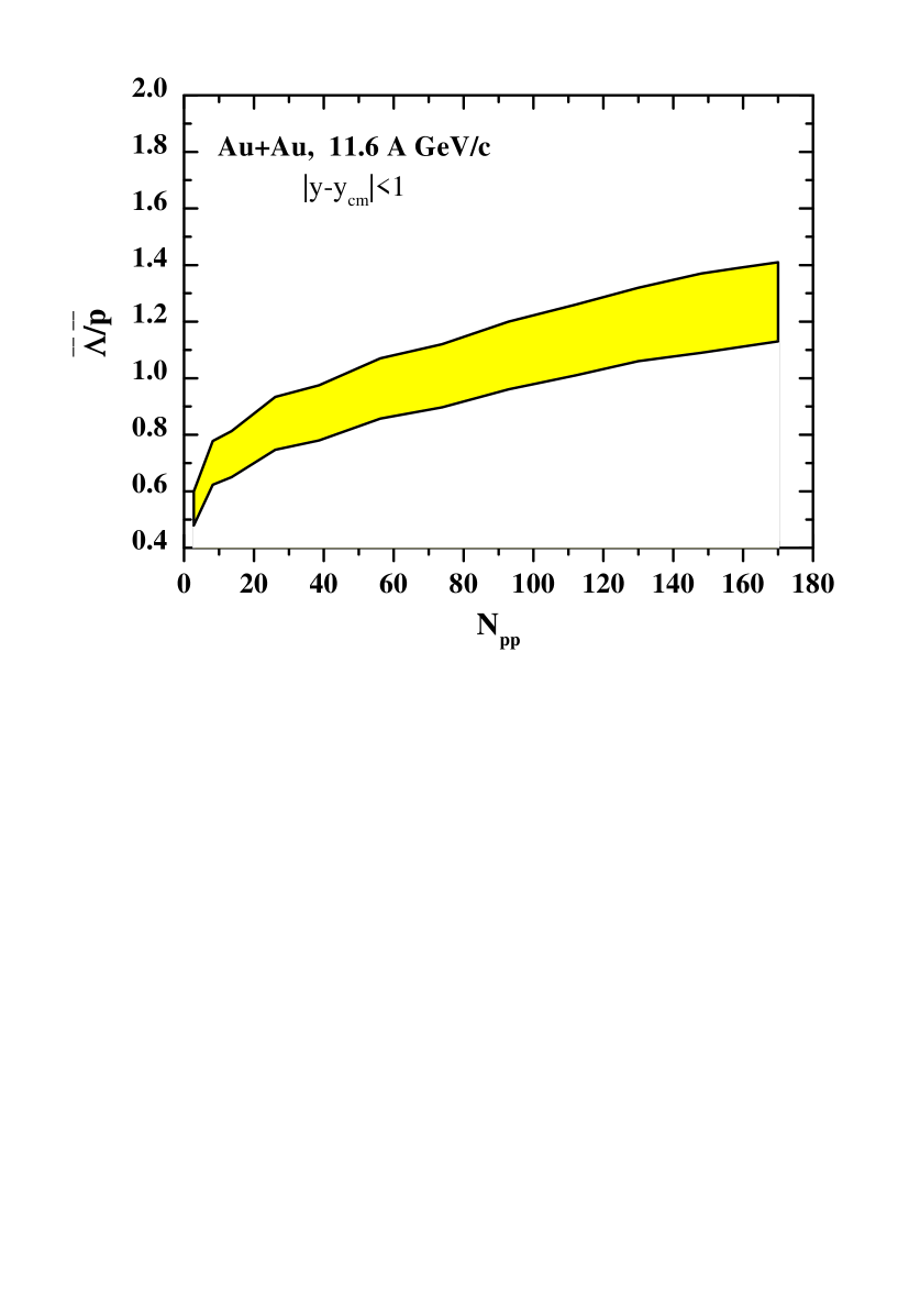
Figure 14: The $\bar{\Lambda}/\bar{p}$ ratio as a function of centrality for $Au+Au$ at 11.6 A$\cdot$GeV/c in the HSD approach within the approximation (51). The shaded area corresponds to the uncertainty in the statistics of the transport calculations for the different particle abundancies at midrapidity.

As mentioned in the introduction, a high ratio of $\bar{\Lambda}$ to $\bar{p}$ of $3.6^{+4.7}_{-1.8}$ has been reported by the E917 Collaboration [28] for central collisions of $Au+Au$ at 11.7 A$\cdot$GeV/c that is not understood so far. These data, furthermore, are in a qualitative agreement with the measurements from the E864/E878 Collaboration [77]. To estimate the $\bar{\Lambda}/\bar{p}$ ratio within the present transport approach as a function of the centrality of the collision we employ again the relation (51) and invoke the particle multiplicities at midrapidity $|\Delta y_{cm}|\leq 1$. The results of these calculations are displayed in Fig. 14 for $Au+Au$ at 11.6 A$\cdot$GeV/c as a function of the number of participating protons indicating a steady rise of the ratio with centrality. The hatched area in Fig. 14 demonstrates the uncertainty in the $\bar{\Lambda}/\bar{p}$ ratio due to the limited statistics. However, the calculations for the most central collisions do not suggest ratios above 1.4 which is still slightly out of the range of the number quoted in Ref. [28] of $3.6^{+4.7}_{-1.8}$. Thus either new theoretical concepts and/or much refined data are necessary to unravel this puzzle.

5 Summary

In this work the conventional transport approach for two-body induced reactions has been extended on the formal level to n-body $n\leftrightarrow m$ reaction channels employing the principles of detailed balance. As a specific example of current interest the baryon-antibaryon annihilation problem in relativistic nucleus-nucleus collisions has been addressed at AGS and SPS energies where the meson densities are comparable (at the AGS) or much larger than the baryon densities (at the SPS) such that multiple meson fusion reactions as suggested in Refs. [22, 50, 51] become very probable.

In order to employ the many-body detailed balance relations (as addressed in Section 2) a simple phase-space model for antibaryon annihilation has been presented that is based on flavor rearrangement channels to pseudoscalar and vector mesons (cf. Fig. 1). Furthermore, a suitable covariant scheme for the calculation of such multi-particle reactions has been presented in Section 3 which is a straight forward extension of the concept proposed by Lang et al. in Ref. [62]. The method and its implementation in the HSD transport approach [20, 54] has been tested for a homogenuous system of nonstrange hadrons in thermal and chemical equilibrium (cf. Fig. 4).

Actual transport calculations have been performed for $Pb+Pb$ at 160 A$\cdot$GeV and $Au+Au$ at 11.6 A$\cdot$GeV/c, i.e. the most prominant reactions at the SPS and the AGS, where a couple of experimental data are available to control the dynamics. It is found that at both energies the meson fusion reactions are by far the most dominant production channel for the final antibaryons (seen experimentally) and that the antibaryons and baryons – at least at midrapidity – come close to local chemical equilibrium with the mesons. As a consequence the $\bar{p}/\pi$ ratio is practically independent on the centrality of the collision, i.e. as a function of $A_{part}$, in line with the experimental observation at both energies.

On the other hand, the approximate chemical equilibration allows to perform rather reliable extrapolations for the strange and multistrange antibaryon abundancies on the basis of particle ratios (cf. (49)), that follow from chemical equilibrium for the mesons and antibaryons. The latter ratios can be calculated with better statistics in the nonperturbative approach than the direct strange antibaryon abundancies. Here a roughly constant $\bar{\Lambda}/\bar{p}$ ratio of $\approx$ 1 is predicted for semi-peripheral to central collisions of $Pb+Pb$ at the SPS that will be controlled soon by experimental data from the NA49 Collaboration. Moreover, a separation of antiprotons from antihyperons will also allow to investigate the question of antiproton self energies that enhance the $\bar{p}/\pi$ ratio with centrality when adopting attractive scalar potentials in line with the analysis performed at SIS energies of $\sim$ 2 A$\cdot$GeV [19]. At AGS energies of 11.6 A$\cdot$GeV/c the situation is less clear due to the rather low statistics for antibaryons, both theoretically and experimentally. Recall that the $\bar{p}/\pi^{+}$ ratio is only about $2.5-3\times 10^{-4}$ at this energy. The HSD transport calculations for the most central collisions of $Au+Au$ at the AGS – assuming (49) to hold – give an upper limit of 1.4 for the $\bar{\Lambda}/\bar{p}$ ratio, which is still slightly out of the range of the number quoted by the E917 Collaboration [28] of $3.6^{+4.7}_{-1.8}$ or related results from Ref. [77]. Thus either new theoretical concepts and/or much refined data will be necessary to unravel the antihyperon puzzle at AGS energies.

The author likes to acknowledge continuous and valuable discussions with C. Greiner. Furthermore, he is indepted to E. L. Bratkovskaya and C. Greiner for critical suggestions and a careful reading of the manuscript.

Figure 1: Illustration of the flavor rearrangement model for $B\bar{B}$ annihilation to 3 mesons and vice versa. The mesons $M_{i}$ may be either pseudo-scalar or vector mesons, respectively.

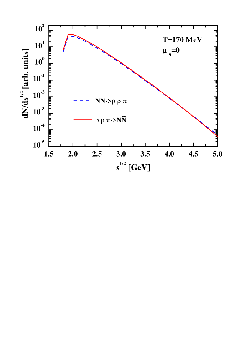
Figure 4: The number of $N\bar{N}\rightarrow\rho\rho\pi$ reactions as a function of the invariant energy $\sqrt{s}$ for a system in thermal and chemical equilibrium at temperature $T$ = 170 MeV and $\mu_{q}$ = 0. The solid line denotes the differential number in the backward ($\rho\rho\pi$) collisions, respectively.

References

- [1] O. Chamberlain et al., Nuovo Cimento 3 (1956) 447.
- [2] T. Elioff et al., Phys. Rev. 128 (1962) 869.
- [3] D. Dorfan et al., Phys. Rev. Lett. 14 (1965) 995.
- [4] A. A. Baldin et al., JETP Lett. 47 (1988) 137.
- [5] J. B. Carroll et al., Phys. Rev. Lett. 62 (1989) 1829.
- [6] A. Shor, V. Perez-Mendez, K. Ganezer, Phys. Rev. Lett. 63 (1989) 2192.
- [7] J. Chiba et al., Nucl. Phys. A 553 (1993) 771c.
- [8] A. Schröter et al., Nucl. Phys. A 553 (1993) 775c.
- [9] G. Batko, W. Cassing, U. Mosel, K. Niita, Phys. Lett. B 256 (1991) 331.
- [10] W. Cassing, A. Lang, S. Teis, K. Weber, Nucl. Phys. A 545 (1992) 123c.
- [11] S. W. Huang, G. Q. Li, T. Maruyama, A. Faessler, Nucl. Phys. A 547 (1992) 653.
- [12] P. Danielewicz, Phys. Rev. C 42 (1990) 1564.
- [13] E. Hernandez, E. Oset, W. Weise, Z. Phys. A 351 (1995) 99.
- [14] J. Schaffner, I. N. Mishustin, L. M. Satarov, H. Stöcker, W. Greiner, Z. Phys. A 341 (1991) 47.
- [15] V. Koch, G. E. Brown, C. M. Ko, Phys. Lett. B 265 (1991) 29.
- [16] S. Teis, W. Cassing, T. Maruyama, U. Mosel, Phys. Rev. C 50 (1994) 388.
- [17] G. Q. Li, C. M. Ko, X. S. Fang, Y. M. Zheng, Phys. Rev. C 49 (1994) 1139.
- [18] C. Spieles, A. Jahns, H. Sorge, H. Stöcker, W. Greiner, Mod. Phys. Lett. A 27 (1993) 2547.
- [19] A. Sibirtsev, W. Cassing, G. I. Lykasov, M. V. Rzjanin, Nucl. Phys. A 632 (1998) 131.
- [20] W. Cassing, E. L. Bratkovskaya, Phys. Rep. 308 (1999) 65.
- [21] C. M. Ko, G. Q. Li, J. Phys. G 22 (1996) 1673.
- [22] C. M. Ko, X. Ge, Phys. Lett. B 205 (1988) 195.
- [23] C. M. Ko, L. H. Xia, Phys. Rev. C 40 (1989) R1118.
- [24] R. Wittmann, PhD thesis, Univ. of Regensburg, 1995; R. Wittmann, U. Heinz, hep-ph/9509328.
- [25] C. B. Dover, T. Gutsche, M. Maruyama, A. Faessler, Prog. Part. Nucl. Phys. 29 (1992) 87.
- [26] L. Ahle et al., Nucl. Phys. A 610 (1996) 139c.
- [27] J. Barrette et al., Phys. Lett. B 485 (2000) 319.
- [28] B. B. Back et al., nucl-ex/0101008.
- [29] G. I. Veres and the NA49 Collaboration, Nucl. Phys. A 661 (1999) 383c.
- [30] J. Bächler et al., Nucl. Phys. A 661 (1999) 45c.
- [31] F. Antinori et al., Nucl. Phys. A 661 (1999) 130c; R. Caliandro et al., J. Phys. G 25 (1999) 171.
- [32] F. Antinori et al., Nucl. Phys. A 681 (2001) 165c; hep-ex/0105049.
- [33] E. Andersen et al., Phys. Lett. B 449 (1999) 401.
- [34] A. Jahns, H. Stöcker, W. Greiner, H. Sorge, Phys. Rev. Lett. 68 (1992) 2895.
- [35] S. H. Kahana, Y. Pang, T. Schlagel, C. B. Dover, Phys. Rev. C 47 (1993) 1356.
- [36] Y. Pang, D. E. Kahana, S. H. Kahana, H. Crawford, Phys. Rev. Lett. 78 (1997) 3418.
- [37] M. Bleicher et al., Phys. Lett. B 485 (2000) 133.
- [38] F. Antinori et al., Eur. Phys. J. C 11 (1999) 79.
- [39] H. Sorge, Z. Phys. C 67 (1995) 479; Phys. Rev. C 52 (1995) 3291.
- [40] K. Werner, J. Aichelin, Phys. Lett. B 308 (1993) 372.
- [41] M. A. Braun, C. Pajares, Nucl. Phys. B 390 (1993) 542; N. Armesto, M. A. Braun, E. G. Ferreiro, C. Pajares, Phys. Lett. B 344 (1995) 301; M. A. Braun, C. Pajares, J. Ranft, Int. Jour. Mod. Phys. A 14 (1999) 2689.
- [42] N. S. Amelin, N. Armesto, C. Pajares, D. Sousa, hep-ph/0103060.
- [43] P. Koch, B. Müller, J. Rafelski, Phys. Rep. 142 (1986) 167.
- [44] P. Braun-Munzinger, I. Heppe, J. Stachel, Phys. Lett. B 465 (1999) 15.
- [45] F. Becattini et al., Phys. Rev. C 64 (2001) 024901.
- [46] F. Becattini, J. Cleymans, A. Keranen, E. Suhonen, K. Redlich, hep-ph/0011322.
- [47] K. Redlich, hep-ph/0105104.
- [48] S. Hamieh, K. Redlich, A. Pounsi, Phys. Lett. B 486 (2000) 61.
- [49] A. Capella, Nucl. Phys. A 661 (1999) 502c.
- [50] R. Rapp, E. Shuryak, Phys. Rev. Lett. 86 (2001) 2980.
- [51] C. Greiner, S. Leupold, nucl-th/0009036.
- [52] E. L. Bratkovskaya, W. Cassing, C. Greiner et al., Nucl. Phys. A 675 (2000) 661.
- [53] L. V. Bravina et al., J. Phys. G 25 (1999) 351; Phys. Rev. C 62 (2000) 064906.
- [54] W. Ehehalt, W. Cassing, Nucl. Phys. A 602 (1996) 449.
- [55] K. Weber et al., Nucl. Phys. A 539 (1992) 713; Nucl. Phys. A 552 (1993) 571; T. Maruyama et al., Nucl. Phys. A 573 (1994) 653.
- [56] W. Botermans, R. Malfliet, Phys. Rep. 198 (1990) 115.
- [57] W. Cassing, V. Metag, U. Mosel, K. Niita, Phys. Rep. 188 (1990) 363.
- [58] W. Cassing, U. Mosel, Prog. Part. Nucl. Phys. 25 (1990) 235.
- [59] W. Cassing, S. Juchem, Nucl. Phys. A 665 (2000) 377; Nucl. Phys. A 672 (2000) 417; Nucl. Phys. A 677 (2000) 445.
- [60] S. Leupold, Nucl. Phys. A 672 (2000) 475.
- [61] E. Byckling, K. Kajantie, Particle Kinematics (John Wiley and Sons, London, 1973).
- [62] A. Lang, H. Babovsky, W. Cassing, U. Mosel, H.-G. Reusch, K. Weber , J. Comp. Phys. 106 (1993) 391.
- [63] H. Schopper (Editor), Landolt-Börnstein, New Series, Vol. I/12, Springer-Verlag, 1988.
- [64] Particle Data Group, Eur. Phys. J. C 15 (2000) 1.
- [65] J. Geiss, W. Cassing, C. Greiner, Nucl. Phys. A 644 (1998) 107.
- [66] Gy. Wolf et al., Nucl. Phys. A 517 (1990) 615; Nucl. Phys. A 552 (1993) 549.
- [67] G. Batko, J. Randrup, T. Vetter, Nucl. Phys. A 536 (1992) 786; Nucl. Phys. A 546 (1992) 761.
- [68] T. Kodama, S. B. Duarte, K. C. Chung et al., Phys. Rev. C 29 (1984) 2146.
- [69] G. F. Bertsch, S. Das Gupta, Phys. Rep. 160 (1988) 189.
- [70] S. Bass et al., Prog. Part. Nucl. Phys. 41 (1998) 225.
- [71] A. B. Larionov, W. Cassing, S. Leupold, U. Mosel, nucl-th/0103019, Nucl. Phys. A, in press.
- [72] I. G. Bearden et al., Nucl. Phys. A 610 (1996) 175c; M. Caneta et al., J. Phys. G 23 (1997) 1865.
- [73] J. Zimanyi, in: S. Bass et al., Nucl. Phys. A 661 (1999) 205c.
- [74] J. Zimanyi, T. S. Biro et al., hep-ph/9904501.
- [75] P. K. Sahu, W. Cassing, U. Mosel, A. Ohnishi, Nucl. Phys. A 672 (2000) 376.
- [76] W. Cassing, E. L. Bratkovskaya, S. Juchem, Nucl. Phys. A 674 (2000) 249.
- [77] T. A. Armstrong et al., Phys. Rev. C 59 (1999) 2699.