Short-range correlations in semi-exclusive electron scattering experiments

S.R. Mokhtar^1,2, M. Anguiano^2,3, G. Co’^2,3 and A.M. Lallena⁴

¹⁾ Department of Physics, University of Assiut,

Assiut, Egypt

²⁾ Dipartimento di Fisica, Università di Lecce,

I-73100 Lecce, Italy

³⁾ Istituto Nazionale di Fisica Nucleare sez. di Lecce,

I-73100 Lecce, Italy

⁴⁾ Departamento de Física Moderna, Universidad de Granada,

E-18071 Granada, Spain

One-nucleon emission electron scattering experiments are studied with a model that considers short–range correlations up to the first order in the number of correlation lines. The proper normalization of the many-body wave functions requires the evaluation of two- and three-point diagrams, the last ones usually neglected in the literature. When all these diagrams are included the effects of the short-range correlations are rather small. The results of our calculations are compared with experimental data taken on ¹⁶O.

PACS number(s): 21.10.Ft, 21.60.-n

1 Introduction

One-nucleon knock out experiments induced by electromagnetic probes have been, and still are, an important tool to study the structure of the atomic nucleus [1, 2]. The main use of these experiments has been the investigation of the ground state single particle structure of nuclei [3]. For this reason, they have been done, in the great majority of cases, in the quasi-elastic region, in order to minimize the effects of the collective nuclear excitations. Nucleon emission in the quasi-elastic region is dominated by the direct knock out of the detected nucleon while the other nucleons behave like spectators. Many-body effects can be treated as corrections to this basic process.

These (e,e’p) experiments have been analyzed in terms of mean field models with great success. The models describe the target nucleus ground state by using a purely real mean field, and the nuclear excited states in terms of one-particle one-hole excitation with the particle moving in a complex optical potential. The optical potential is usually taken from a fit to proton elastic scattering data off the A-1 nucleus. This approach reproduces rather well the behavior of the cross section in terms of the so-called missing momentum. What remains, however, is the problem of the overestimation of its magnitude. The quenching factor necessary to reproduce the data has been related to the spectroscopic factor which nowadays has achieved the same status as a true observable [4].

The increased accuracy of the data as well as the possibility of performing more elaborate numerical calculations, has stressed the need for better descriptions of (e,e’p) data. The source of the spectroscopic factor has been investigated following various hypotheses, from relativistic effects [5] to in medium modifications of the nucleon properties [6]. At the moment, one of the most frequently considered hypotheses is the partial occupation of the single particle levels produced by the short-range correlations [7]. Various estimates of these occupation probabilities have been done both in nuclear matter [8, 9] and in finite nuclei [10, 11], but their values do not seem to be compatible with the empirical spectroscopic factors. On the other hand, direct calculations of (e,e’p) cross sections with models taking into account short-range correlations show noticeable effects produced by these correlations [12]-[15], in spite of the fact that also in these cases spectroscopic factors are still needed. These calculations of the semi-inclusive cross section have been done with simplified treatments of the correlations. In some calculations only the lowest order cluster terms have been considered [12, 13, 15]. In other calculations [14] the overlap wave function, which in the mean field model corresponds to the hole single particle wave function, has been extracted from correlated one-body density distributions evaluated via more or less sophisticated ground state calculations.

There are two weak points in these calculations. A first one concerns the inconsistency of the various inputs of the calculations. Single particle wave functions and correlations are not linked by a unique nuclear hamiltonian as they should be. The second weak point is related to the fact that the proper normalization of the many-body wave function is not preserved.

We have developed a model which takes into account all the diagrams containing a single correlation line [16]. Since the cluster expansion conserves the sum rules order by order [17], the normalization of the wave function is maintained. This is immediately seen in the application of the model to the description of the ground state densities [18, 19]. The validity of our model has been tested in nuclear matter by comparing our results with those obtained in a calculation that considers all the cluster terms [20]. The agreement between the two results is excellent, showing that, for relatively simple operators, like the charge operator, the first order approximation is reliable.

The inputs of our model, single particle wave functions and correlations, are taken from Fermi Hypernetted Chain (FHNC) calculations of the ground state of closed shell nuclei obtained by minimizing the hamiltonian expectation value evaluated with realistic and semi-realistic nucleon-nucleon potentials [21, 22].

In this paper we present the results of our investigation of (e,e’p) reactions in ¹⁶O. We have analyzed the validity of various approximations commonly adopted in the mean field description of these processes. It is not at all evident that approximations which are within a certain theoretical framework should remain valid in a different one. Moreover, if the aim is to disentangle subtle physical effects, the uncertainty in the result due to some adopted assumption can be comparable with the magnitude of the searched effect.

Summarizing in few words our findings we may say that short-range correlation effects are extremely small and cannot explain the values of spectroscopic factors needed to reproduce the data.

2 The cross section

In this section we briefly recall the expressions of the coincidence cross section used in our calculations. We work in natural units ($\hbar=c=1,e^{2}=1/137.04$) and employ the conventions of Bjorken and Drell [23]. The initial and final electron four vectors are respectively $k\equiv(\epsilon,{\bf k})$ and $k^{\prime}\equiv(\epsilon^{\prime},{\bf k}^{\prime})$, and we used the symbol $q\equiv(\omega,{\bf q})=k-k^{\prime}$ to indicate the four momentum transfer. The four momentum of the emitted nucleon is $p\equiv(\epsilon_{p},{\bf p})$. The reference system, shown in Fig. 1, has been defined following the commonly used prescriptions. The scattering plane is defined by the electron vectors ${\bf k}$ and ${\bf k}^{\prime}$, $\theta$ is the angle of the scattered electron, the quantization axis is taken along the direction of ${\bf q}$, and the angle $\theta_{p}$ and $\phi_{p}$ define the direction of the emitted nucleon.

Figure 1: Reference system used in our calculations.

In our calculations the cross section has been derived by adopting the commonly used assumptions [24]: the electron wave functions are plane wave solutions of the Dirac equation, only one photon is exchanged between the electron and the nucleus, all the terms depending upon the electron rest mass are neglected. With these approximations we obtain:

$$\frac{{\rm d}^{6}\sigma}{{\rm d}\epsilon^{\prime}{\rm d}\Omega_{e}{\rm d}\epsilon_{p}{\rm d}\Omega_{p}}=\frac{\sigma_{M}K}{(2\pi)^{3}}\left(v_{l}w_{l}+v_{t}w_{t}+v_{tl}w_{tl}+v_{tt}w_{tt}\right)\,,$$ (1)

where we have indicated with $\sigma_{M}$ the Mott cross section:

$$\sigma_{M}\,=\,\left(\frac{e^{2}\cos(\theta/2)}{2\epsilon_{i}\sin^{2}(\theta/2)}\right)^{2}$$ (2)

Since we describe the emitted particle within the non relativistic kinematics, we obtain $K=|{\bf{p}}|m_{p}$. The factors $v$ come from the leptonic tensor and depend only from kinematic variables:

$$v_{l} = \left(\frac{q_{\mu}^{2}}{{\bf q}^{2}}\right)^{2}\,,$$ (3)

$$v_{t} = \tan^{2}\frac{\theta}{2}-\frac{1}{2}\frac{q_{\mu}^{2}}{{\bf q}^{2}}\,,$$ (4)

$$v_{tl} = \frac{q_{\mu}^{2}}{\sqrt{2}{\bf q}^{2}}\,\left(\tan^{2}\frac{\theta}{2}-\frac{q_{\mu}^{2}}{{\bf q}^{2}}\right)^{\frac{1}{2}}\,,$$ (5)

$$v_{tt} = \frac{1}{2}\frac{q_{\mu}^{2}}{{\bf q}^{2}}\,.$$ (6)

The information about the nuclear structure is included in the $w$ factors. Because of the current conservation only three components of the current four-vector are independent. We choose the charge $\rho({\bf q})$ and the two transverse components in spherical coordinates:

$$J_{\pm}=\mp\frac{1}{\sqrt{2}}\left(J_{x}\pm iJ_{y}\right)\,.$$ (7)

We can express the $w$ factors as [25, 26]:

$$w_{l} = \langle\Psi_{i}|\rho^{\dagger}({\bf q})|\Psi_{f}\rangle\langle\Psi_{f}|\rho({\bf q})|\Psi_{i}\rangle\,,$$ (8)

$$w_{t} = \langle\Psi_{i}|J_{-}^{\dagger}({\bf q})|\Psi_{f}\rangle\langle\Psi_{f}|J_{-}({\bf q})|\Psi_{i}\rangle+\langle\Psi_{i}|J_{+}^{\dagger}({\bf q})|\Psi_{f}\rangle\langle\Psi_{f}|J_{+}({\bf q})|\Psi_{i}\rangle\,,$$ (9)

$$w_{tl} = 2Re\left(\langle\Psi_{i}|\rho^{\dagger}({\bf q})|\Psi_{f}\rangle\langle\Psi_{f}|J_{-}({\bf q})|\Psi_{i}\rangle-\langle\Psi_{i}|\rho^{\dagger}({\bf q})|\Psi_{f}\rangle\langle\Psi_{i}|J^{\dagger}_{+}({\bf q})|\Psi_{f}\rangle\right)\,,$$ (10)

$$w_{tt} = 2Re\left(\langle\Psi_{i}|J^{\dagger}_{+}({\bf q})|\Psi_{f}\rangle\langle\Psi_{f}|J_{-}({\bf q})|\Psi_{i}\rangle\right)\,,$$ (11)

where we have indicated with $|\Psi_{i}\rangle$ and $|\Psi_{f}\rangle$ initial and final states of the full hadronic system. In the previous equations a sum on $\sigma$ and $m_{h}$ the projection on the z axis of the spin of the emitted particle and of the angular momentum of the the residual nucleus it is understood.

In this work we consider only one-body electromagnetic currents. The charge operator is expressed as:

$$\rho({\bf r})\,=\,\sum^{A}_{k=1}\frac{1+\tau^{3}_{k}}{2}\,\delta({\bf r}-{\bf r}_{k})\,,$$ (12)

the convection current operator as:

$$J^{\rm C}({\bf r})\,=\,\sum^{A}_{k=1}\frac{-i}{2M_{k}}\,\frac{1+\tau^{3}_{k}}{2}\,\left[\delta({\bf r}-{\bf r}_{k})\nabla_{k}-\nabla_{k}\delta({\bf r}-{\bf r}_{k})\right]\,,$$ (13)

and the magnetization current operator as:

$$J^{\rm M}({\bf r})\,=\,\sum^{A}_{k=1}\frac{1}{2M_{k}}\,\left(\mu^{\rm P}\frac{1+\tau^{3}_{k}}{2}+\mu^{\rm N}\frac{1-\tau^{3}_{k}}{2}\right)\nabla\times\delta({\bf r}-{\bf r}_{k})\,\mbox{\boldmath$\sigma$}_{k}\,.$$ (14)

In the previous equations $M_{k}$ indicates the rest mass of $k$–th nucleon, $\mu^{\rm P}$ and $\mu^{\rm N}$ the anomalous magnetic moment of the proton and the neutron respectively, $\mbox{\boldmath$\sigma$}_{k}$ the Pauli spin matrix of the k–th nucleon and $\tau^{3}_{k}=1$ ($-1$) for protons (neutrons). In our calculations the nucleonic internal structure has been considered by folding the point-like responses with the electromagnetic nucleon form factors of Ref. [27].

3 The nuclear model

The nuclear final state $|\Psi_{f}\rangle$ is described in the asymptotic region as the product of the wave functions of the emitted nucleon, $\phi({\bf p}\cdot{\bf r})\chi_{\sigma}$, with ${\bf p}$ its momentum, and of the rest nucleus, $\Psi({\bf r}_{1}...{\bf r}_{A-1};\epsilon_{h};j_{h},m_{h})$. We have indicated with $j_{h}$ the angular momentum of the rest nucleus and we have defined $\epsilon_{h}=\epsilon_{p}-\omega$. In a strict independent particle model these quantities correspond to the energy and angular momentum of the hole state. We perform a multipole expansion of $|\Psi_{f}\rangle$ to express it in terms of eigenstates of the total angular momentum of the A nucleon system:

$$|\Psi_{f}\rangle = \frac{4\pi}{|{\bf p}|}\sum_{l_{p}\mu_{p}}\sum_{j_{p}m_{p}}\sum_{JM,\Pi}i^{l_{p}}Y^{*}_{l_{p}\mu_{p}}(\widehat{\bf p})\langle l_{p}\mu_{p}\frac{1}{2}\sigma|j_{p}m_{p}\rangle$$ (15)

$$\langle j_{p}m_{p}j_{h}m_{h}|JM\rangle|\Psi;JM,\Pi;(l_{p}j_{p}m_{p}\epsilon_{p},l_{h}j_{h}m_{h}\epsilon_{h})\rangle$$

$$\equiv \frac{4\pi}{|{\bf p}|}\sum_{p}\sum_{JM,\Pi}i^{l_{p}}Y^{*}_{l_{p}\mu_{p}}(\widehat{\bf p})\langle l_{p}\mu_{p}\frac{1}{2}\sigma|j_{p}m_{p}\rangle$$

$$\langle j_{p}m_{p}j_{h}m_{h}|JM\rangle\,\,\frac{|JM,\Pi;p,h\rangle}{\langle JM,\Pi;p,h|JM,\Pi;p,h\rangle^{\frac{1}{2}}}\,.$$

In the above equations the state $|\Psi;JM,\Pi;(l_{p}j_{p}m_{p}\epsilon_{p},l_{h}j_{h}m_{h}\epsilon_{h})\rangle$ represents the excited state of the system with A nucleons with total angular momentum $J$ projection $M$, parity $\Pi$, having a particle in the continuum wave characterized by orbital and total angular momentum $l_{p}$ and $j_{p}$ with projection $m_{p}$ and energy $\epsilon_{p}$, and a residual nucleus with hole quantum numbers $l_{h}$ $j_{h}$, $m_{h}$ and $\epsilon_{h}$. We have indicated with $Y_{l\mu}$ the spherical harmonics and with the symbol $\langle l_{a}m_{a}l_{b}m_{b}|JM\rangle$ the Clebsch-Gordan coefficients [28]. In the last expression, the nuclear excited state is given in terms of unnormalized many-body wave function $|JM,\Pi;p,h\rangle$

In our model, the nuclear final state with total angular momentum $J$ is described as a superposition of all possible one-particle one-hole transitions allowed by the angular momentum selection rules. Within this approximation, the knowledge of the energy and of the momentum of the emitted nucleon determines the quantum numbers of the hole state of the residual nucleus. Then the summation on the hole states drops and we sum only over the possible particle states in the continuum. We defined the sum over $p$ as a summation over the $l_{p}$, $\mu_{p}$, $j_{p}$ and $m_{p}$ quantum numbers.

From the equations (8)-(11) defining the $w$ factors, one can see that the basic ingredients to be calculated are the transition matrix elements from the ground state to the excited state of the nuclear system induced by a one body operator. We write the transition matrix elements as:

$$\langle\Psi_{f}|O_{\eta}({\bf q})|\Psi_{i}\rangle = \frac{4\pi}{|{\bf p}|}\sum_{p}\sum_{J,M,\Pi}(-i)^{l_{p}}Y_{l_{p}\mu_{p}}(\widehat{\bf p})\langle l_{p}\mu_{p}\frac{1}{2}\sigma|j_{p}m_{p}\rangle\langle j_{p}m_{p}j_{h}m_{h}|JM\rangle$$ (16)

$$\frac{\langle JM,\Pi;p,h|O_{\eta}({\bf q})|00,+1\rangle}{\langle JM,\Pi;p,h|JM,\Pi;p,h\rangle^{\frac{1}{2}}\langle 00,+1|00,+1\rangle^{\frac{1}{2}}}$$

$$\equiv \frac{4\pi}{|{\bf p}|}\sum_{p}\sum_{J,M,\Pi}{\cal A}(p,h;J,M,\Pi)\,\,\xi_{J,M,\eta,\Pi}({\bf q};p,h)\,,$$

where $|00,+1\rangle$ is the unnormalized ground state which, for the nuclei we shall consider, has zero angular momentum and positive parity. We have included all the geometric part of the expression in the symbol

$${\cal A}(p,h;J,M,\Pi)=(-i)^{l_{p}}Y_{l_{p}\mu_{p}}(\widehat{\bf p})\langle l_{p}\mu_{p}\frac{1}{2}\sigma|j_{p}m_{p}\rangle\langle j_{p}m_{p}j_{h}m_{h}|JM\rangle\,,$$ (17)

and we have indicated with $O_{\eta}({\bf q})$ the generic one-body operator inducing the transition. For $\eta=0$ this is the charge operator, while for $\eta=\pm 1$ is given by the appropriate sum of convection and magnetization currents, Eq. (7).

In our nuclear model we consider the nuclear states described as:

$$|00,+1\rangle = F\,\,|\Phi;00,+1\rangle\,,$$ (18)

$$|JM,\Pi;p,h\rangle = F\,\,|\Phi;JM,\Pi;p,h\rangle\,.$$ (19)

We have indicated with $|\Phi;00,+1\rangle$ the Slater determinant describing the mean field wave function in a pure independent particle model. This means that, taken a basis of single particle wave functions, all the states below the Fermi surface are fully occupied and those above all completely empty. The state $|\Phi;JM,\Pi;ph\rangle$ indicates a Slater determinant where the hole function $h$ has been substituted with the continuum particle function $p$. With respect to a pure independent particle model, the novelty is the presence of the correlation function F. This function has, in principle, a very complicated operatorial dependence, analogous to that of the hamiltonian. Our calculations have been restricted to the use of purely scalar (Jastrow) correlations. For this reason we immediately simplify the expressions formulating them only in terms of this type of correlations. The adopted ansatz on the correlation is:

$$F(1,2,...A)=\prod^{A}_{i<j}f(r_{ij})\,,$$ (20)

where $r_{ij}=|{\bf r}_{i}-{\bf r}_{j}|$ is the distance between the positions of the particles $i$ and $j$.

Using the well-known cluster expansion techniques we rewrite the transition matrix $\xi_{J,M,\eta,\Pi}({\bf q};p,h)$ in Eq. (16) as:

$$\xi_{J,M,\eta,\Pi}({\bf q};p,h)=\frac{\langle JM,\Pi;p,h|O_{\eta}({\bf q})|00,+1\rangle}{\langle 00,+1|00,+1\rangle}\left[\frac{\langle 00,+1|00,+1\rangle}{\langle JM,\Pi;p,h|JM,\Pi;p,h\rangle}\right]^{\frac{1}{2}}\,.$$ (21)

The two factors in Eq. (21) are separately evaluated by expanding both numerator and denominator in powers of the short-range correlation function. The presence of the denominators is used to eliminate the unlinked diagrams [29].

Since in our calculations the correlation functions are purely scalar they commute with the operator $O_{\eta}({\bf q})$ and therefore we have to deal with terms of the kind:

$$\langle JM,\Pi;p,h|O_{\eta}({\bf q})|00,+1\rangle = \langle\Phi;JM,\Pi;p,h|F^{\dagger}O_{\eta}({\bf q})F|\Phi;00,+1\rangle_{L}$$ (22)

$$= \langle\Phi;JM,\Pi;p,h|O_{\eta}({\bf q})\prod^{A}_{i<j}f^{2}(r_{ij})|\Phi;00,+1\rangle_{L}$$

$$= \langle\Phi;JM,\Pi;p,h|O_{\eta}({\bf q})\prod^{A}_{i<j}(1+h_{ij})|\Phi;00,+1\rangle_{L}\,,$$

where we have used the function $h_{ij}=f^{2}(r_{ij})-1$ and the subindex $L$ indicates that only the linked diagrams are considered.

The approximation of our model consists in retaining only those terms where the $h_{ij}$ function appears only once:

$$\xi_{J,M,\eta,\Pi}({\bf q};p,h) \longrightarrow \xi^{1}_{J,M,\eta,\Pi}({\bf q};p,h)$$ (23)

$$\,=\, \langle\Phi;JM,\Pi;p,h|\,O_{\eta}({\bf q})\,\sum_{i<j}\,(1+h_{ij})\,|\Phi;00,+1\rangle_{L}\,.$$

This result has been obtained using a procedure analogous to that adopted in Ref. [18] for the evaluation of the density distribution, and therefore the truncation of the expansion is done only after the elimination of the unlinked diagrams.

We show in Fig. 2 the Mayer like diagrams describing all the terms considered in our calculations. This set of diagrams has already been presented elsewhere [16, 20], but we show them again because the identification of the individual diagrams is essential for the discussion of the results. In each diagram the black square indicates the coordinate where the one-body operator $O_{\eta}({\bf q})$ is acting, while the black dots indicate the other coordinates. The dashed line represents the correlation function $h_{ij}$, which operates on two-coordinates only, and the continuous oriented lines the single particle wave functions $\phi_{k}$.

Figure 2: Mayer-like diagrams considered. The black squares represent the point where the external field is acting on, the dashed line the correlation function and the oriented lines the single particle wave functions.

If we label with $1$ the coordinate where the external operator $O({\bf q})$ is acting, we can specify the $\xi^{1}$ of Eq. (23) as:

$$\xi^{1}_{J,M,\eta,\Pi}({\bf q};p,h)\, = \,\langle\Phi;JM,\Pi;p,h|\,O_{\eta}({\bf q})\,|\Phi;00,+1\rangle$$

$$+\,\langle\Phi;JM,\Pi;p,h|\,O_{\eta}({\bf q})\,\sum^{A}_{j>1}\,h_{1j}\,|\Phi;00,+1\rangle_{L}$$

$$+\,\langle\Phi;JM,\Pi;p,h|\,O_{\eta}({\bf q})\,\sum^{A}_{1<i<j}\,h_{ij}\,|\Phi;00,+1\rangle_{L}\,.$$ (24)

The above expression shows that our model generates, in addition to the uncorrelated transitions represented in Fig. 2 by the one-point diagram (1.1), also two- and three-point diagrams. The presence of these last diagrams is necessary to have the correct normalization of the many-body wave function, as discussed in [16].

In our case the operators $O_{\eta}({\bf q})$ are the Fourier transforms of the charge and current operators $O_{\eta}({\bf r})$ given in Eqs. (12)-(14). Since we describe the nuclear transition between states with good angular momentum, it is convenient to make a multipole expansions of these operators. For the charge we have:

$$M_{JM}(q)\,=\,\int{\rm d}^{3}r\,j_{J}(qr)\,Y_{JM}(\hat{{\bf r}})\,\rho({\bf r})\,,$$ (25)

where we have indicated with $\hat{{\bf r}}$ the $\theta$ and $\phi$ angles characterizing the vector ${\bf r}$ in polar coordinates and with $j_{J}$ the spherical Bessel functions.

For the current we should distinguish between the electric excitations (E), with natural parity $\Pi=(-1)^{J}$, and the magnetic excitations (M), with unnatural parity $\Pi=(-1)^{J+1}$:

$$T^{\rm E}_{JM}(q)\,=\,\frac{1}{q}\,\int{\rm d}^{3}r\,\left\{\nabla\times\left[j_{J}(qr)\,{\bf Y}^{M}_{JJ}(\hat{{\bf r}})\right]\right\}\cdot{\bf J}({\bf r})$$ (26)

and

$$T^{\rm M}_{JM}(q)\,=\,\int{\rm d}^{3}r\,j_{J}(qr)\,{\bf Y}^{M}_{JJ}(\hat{{\bf r}})\cdot{\bf J}({\bf r})\,,$$ (27)

where we have used the symbol ${\bf Y}^{M}_{JJ}$ to indicate the vector spherical harmonics [28].

By substituting the above equations into Eq. (16) and using the Wigner-Eckart theorem and the properties of the 3j symbols, we can rewrite Eq. (16) in terms of reduced matrix elements:

$$\langle\Psi_{f}|O_{\eta}({\bf q})|\Psi_{i}\rangle = \frac{4\pi}{|{\bf p}|}\sum_{p}\sum_{J,M,\Pi}{\cal A}(p,h;J,M,\Pi)\,\,\xi^{1}_{J,M,\eta,\Pi}({\bf q};p,h)$$

$$= \frac{4\pi}{|{\bf p}|}\sum_{p}\sum_{J,\Pi}{\cal A}(p,h;J,-\eta,\Pi)\,\,$$

$$\times(-i)^{-J}\sqrt{2\pi}\biggl{[}\langle\Phi;J,\Pi;p,h||\,O_{J(\eta)}({\bf q})\,||\Phi;0,+1\rangle$$

$$+\,\langle\Phi;J,\Pi;p,h||\,O_{J(\eta)}({\bf q})\,\sum^{A}_{j>1}\,h_{1j}\,||\Phi;0,+1\rangle$$

$$+\,\langle\Phi;J,\Pi;p,h||\,O_{J(\eta)}({\bf q})\,\sum^{A}_{1<i<j}\,h_{ij}\,||\Phi;0,+1\rangle\biggr{]}\,,$$ (28)

where we have defined the operators:

$$O_{J(\eta)}({\bf q})=\left\{\begin{array}[]{ll}\sqrt{2}M_{J(0)}(q)&\textrm{if $\eta=0$}\\ T^{\rm E}_{J(\pm 1)}(q)+\eta T^{\rm M}_{J(\pm 1)}(q)&\textrm{if $\eta=\pm 1$}\end{array}\right.\,.$$ (29)

In Eq. (28) the sum on M drops because $M=-\eta$ due to angular momentum conservation.

Following Ref. [16] the calculations of the transition matrix elements are carried out by performing a multipole expansion of the correlation function $h_{ij}$:

$$h_{ij}\,=\,h(r_{ij})\,=\,h(r_{i},r_{j},\cos\theta_{ij})\,=\,\sum_{L=0}^{\infty}\,h_{L}(r_{i},r_{j})\,P_{L}(\cos\theta_{ij})\,,$$ (30)

where $P_{L}$ are the associated Legendre polynomials.

The final state quantum numbers are determined by the quantum numbers of the uncorrelated many body state $|\Phi^{\Pi}_{JM}\rangle$ built as a Slater determinant of single particle wave functions of the form:

$$\phi_{k}({\bf r})\,\equiv\,R^{t}_{n_{k}l_{k}j_{k}}(r)\,\sum_{\mu_{k}s}\,\langle l_{k}\mu_{k}\frac{1}{2}s|j_{k}m_{k}\rangle\,Y_{l_{k}\mu_{k}}(\hat{{\bf r}})\,\chi_{s}\,\chi_{t}\,,$$ (31)

where $\chi_{s}$ and $\chi_{t}$ are the spin and isospin wave functions respectively.

By using the orthonormality of the single particle basis, we rewrite Eq. (28) as:

$$\langle\Psi_{f}|O_{\eta}({\bf q})|\Psi_{i}\rangle = \frac{4\pi\sqrt{2\pi}}{|{\bf p}|}\sum_{p}\sum_{J,\Pi}(-i)^{-J}{\cal A}(p,h;J,-\eta,\Pi)\,\,$$

$$\times\biggl{[}\langle p||\,O_{J(\eta)}({\bf q})\,||h\rangle\,+\,\sum_{j}\,\langle p,j||\,O_{J(\eta)}({\bf q})\,h_{12}\,||h,j\rangle$$

$$+\,\sum_{jk}\,\langle p,j,k||\,O_{J(\eta)}({\bf q})\,h_{23}\,||h,j,k\rangle\biggr{]}$$ (32)

$$= \frac{4\pi\sqrt{2\pi}}{|{\bf p}|}\sum_{ph}\sum_{J,\Pi}(-i)^{-J}{\cal A}(p,h;J,-\eta,\Pi)\,\,\xi^{1}_{J,\eta,\Pi}({\bf q};p,h)\,,$$

where $\xi^{1}_{J,\eta,\Pi}({\bf q};p,h)$ is the sum of the reduced matrix elements corresponding to the one-, two- and three-points diagrams. Here the sums of the $j$ and $k$ indices are running on all the hole single particle wave functions. The subindices $1,2,3$ of the correlation function $h$ are associated with the radial coordinates of the first wave function, where also $O_{J(\eta)}({\bf q})$ is acting, the second and the third one respectively. We have indicated only the direct matrix elements in the second and third term of the equation, but we calculate all the exchange diagrams, as shown in Fig. 2.

The multipoles of the one-body operators are calculated by inserting the expressions (12), (13) and (14) into Eqs. (25), (26) and (27). Generally, one may write the resulting operator $O^{1}_{JM}({\bf q})$ as the product of a term depending on $q$ and on the modulus of ${\bf r}_{1}$ times a term depending only on the angular coordinates:

$${O}^{1}_{JM}({\bf q})\equiv F_{J}(qr_{1}){\cal O}_{JM}(\hat{{\bf r}}_{1})\,.$$ (33)

The evaluation of the matrix elements of the various diagrams for the three operators follows the lines of Ref. [16]. In the present calculation we have added all the correlated diagrams of the convection current, which in that reference was included only at the mean field level.

All the ingredients needed to calculate the cross section are now available. The information on the angular distribution of the emitted particle is fully contained in the spherical harmonics of Eq. (17), which has to be squared to calculate the response. We have to deal with a geometrical term of the type:

$$\biggl{(}(-i)^{-J^{\prime}}{\cal A}(p^{\prime},h^{\prime};J^{\prime},-\eta^{\prime},\Pi^{\prime})\biggr{)}^{*}\,\,\biggl{(}(-i)^{-J}{\cal A}(p,h;J,-\eta,\Pi)\biggr{)}\,=$$ (34)

$$= \langle l_{p}^{\prime}(-m_{h}-\eta^{\prime}-\sigma)\frac{1}{2}\sigma|j_{p}^{\prime}(-m_{h}-\eta^{\prime})\rangle\langle j_{p}^{\prime}(-m_{h}-\eta^{\prime})j_{h}m_{h}|J^{\prime}-\eta^{\prime}\rangle$$

$$\langle l_{p}(-m_{h}-\eta-\sigma)\frac{1}{2}\sigma|j_{p}(-m_{h}-\eta)\rangle\langle j_{p}(-m_{h}-\eta)j_{h}m_{h}|J-\eta\rangle$$

$$(-i)^{l_{p}-l_{p}^{\prime}-J+J^{\prime}}Y_{l_{p},(-m_{h}-\eta-\sigma)}(\widehat{\bf p})Y^{*}_{l_{p}^{\prime},(-m_{h}-\eta^{\prime}-\sigma)}(\widehat{\bf p})\,.$$

This expression arises because the angular momentum of the hole $j_{h}$ , its z axis projection $m_{h}$, and $\sigma$ the third component of the spin of the emitted particle, are good quantum numbers of the hadronic final state. The above equation shows that the dependence from the angle $\phi_{p}$ between the scattering plane and the plane where the momentum of the emitted particle is lying, is present only when $\eta\neq\eta^{\prime}$, i.e. only in the interference terms $tl$ and $tt$ in Eq. (1).

We rewrite the cross section expression as:

$$\frac{d^{6}\sigma}{d\epsilon^{\prime}d\Omega_{e}dE^{\prime}d\Omega_{p}} = \frac{\sigma_{M}K}{(2\pi)^{3}}\left[v_{l}W_{0,0}+v_{t}(W_{+1,+1}+W_{-1,-1})\right.$$ (35)

$$\left.+2v_{tl}Re(W_{0,-1}-W_{0,+1})\cos\phi_{p}+2v_{tt}Re(W_{+1,-1})\cos 2\phi_{p}\right],$$

where the $W$ functions are defined as [25]:

$$W_{\eta\eta^{\prime}} = \frac{32\pi^{3}}{|{\bf p}|^{2}}\sum_{\sigma m_{h}}\sum_{J\Pi l_{p}j_{p}}\sum_{J^{\prime}\Pi^{\prime}l_{p}^{\prime}j_{p}^{\prime}}(-i)^{l_{p}-l_{p}^{\prime}-J+J^{\prime}}(-1)^{\eta-\eta^{\prime}}$$ (36)

$$\langle l_{p}(-m_{h}-\eta-\sigma)\frac{1}{2}\sigma|j_{p}(-m_{h}-\eta)\rangle\langle j_{p}(-m_{h}-\eta)j_{h}m_{h}|J-\eta\rangle$$

$$\langle l_{p}^{\prime}(-m_{h}-\eta^{\prime}-\sigma)\frac{1}{2}\sigma|j_{p}^{\prime}(-m_{h}-\eta^{\prime})\rangle\langle j_{p}^{\prime}(-m_{h}-\eta^{\prime})j_{h}m_{h}|J^{\prime}-\eta^{\prime}\rangle$$

$$\left[\frac{(l_{p}+m_{h}+\eta+\sigma)!}{(l_{p}-m_{h}-\eta-\sigma)!}\frac{(l_{p}^{\prime}+m_{h}+\eta^{\prime}+\sigma)!}{(l_{p}^{\prime}-m_{h}-\eta^{\prime}-\sigma)!}\right]^{\frac{1}{2}}\left[\frac{2l_{p}+1}{4\pi}\right]^{\frac{1}{2}}\left[\frac{2l_{p}^{\prime}+1}{4\pi}\right]^{\frac{1}{2}}$$

$$P^{-m_{h}-\eta-\sigma}_{l_{p}}(\cos\theta_{p})\,\,P^{-m_{h}-\eta^{\prime}-\sigma}_{l_{p}^{\prime}}(\cos\theta_{p})$$

$$\xi^{1}_{J,\eta,\Pi}({\bf q};p,h)\,\,\xi^{1\dagger}_{J^{\prime},\eta^{\prime},\Pi^{\prime}}({\bf q};p^{\prime},h)\,.$$

4 Specific applications

We have applied our model to the investigation of the ¹⁶O(e,e’p)¹⁵N reaction in the quasi-elastic region. This nucleus has been chosen for two main reasons. The first one because it is a sufficiently light nucleus, such that the plane wave description of the electron wave functions is still valid [30]. The second reason is related to the fact that this nucleus has been studied with microscopic theories that provide us the needed input for our calculations. Specifically, the single particle bases and the correlation functions are taken from Ref. [21] and [22] where they have been fixed by minimizing microscopic many body hamiltonians. The calculations of Ref. [21] have been done with the semi-realistic nuclear interaction S3 of Afnan and Tang [31] by using a purely scalar correlation function. The calculations of Ref. [22] have been done with a reduction of the Argonne V18 interaction [32] called V8’ and used to perform Green function Monte Carlo calculations [33]. In [22] a complicated state dependent correlation functions was used, while in the calculations of the present paper we have considered only the scalar term of this correlation. These two inputs are the same used in Ref. [16] to calculate the inclusive responses, and as in that case we shall label with S3 and V8 the results obtained respectively with them. For sake of completeness we give in Table 1 the parameters of the Woods-Saxon potentials and we show in Fig. 3 the two correlation functions used. If not specifically mentioned our results have been obtained by using the same mean field for particle and hole states. We shall investigate in Sect. 4.2 the effect of using different mean fields as it is commonly done in the investigation of (e,e’p) data.

Figure 3: Correlation functions used in our calculations.

Table 1: Parameters of the Woods-Saxon potentials used to generate the set of single particle wave functions.

		V8	S3
$\pi$	$V_{0}$ [MeV]	-53.0	-52.5
	$V_{ls}$ [MeV]	0.0	-7.0
	$R$ [fm]	3.45	3.2
	$a$ [fm]	0.7	0.53
$\nu$	$V_{0}$ [MeV]	-53.0	-52.5
	$V_{ls}$ [MeV]	0.0	-6.54
	$R$ [fm]	3.45	3.2
	$a$ [fm]	0.7	0.53

Our calculations have been done in both perpendicular and parallel kinematics. In the first situation the value of the momentum transfer ${\bf q}$ is kept fixed and the changes of $p_{i}=|{\bf p}-{\bf q}|$, the momentum of the proton before being emitted, are obtained by changing the detection angle $\theta_{p}$. This is, for us, the easiest case to calculate and to investigate, even though all the four response functions $W_{\eta\eta^{\prime}}$ contribute. In the second situation, the parallel kinematics, the momentum transfer ${\bf q}$ and the momentum of the emitted nucleon ${\bf p}$ are kept in the same direction and the missing momentum is changed by changing the values of ${\bf q}$. In this case the interference responses, those with $\eta\neq\eta^{\prime}$ do not contribute [25].

Since in (e,e’p) processes the number of variables into play is relatively large, we have mainly done our investigation at a fixed value of $\omega=\epsilon_{i}-\epsilon_{f}$ = 128 MeV, and for a fixed value of momentum of the emitted proton, $|{\bf p}|$= 444 MeV/c, knocked out from the 1p_1/2 level. In perpendicular kinematics the scattering angle was fixed to set ${\bf q}={\bf p}$, to be able to scan all the values of $p_{i}$ from 0 up to 2${\bf q}$. The kinematical conditions just described correspond, for the perpendicular kinematics, to those of experimental data of Ref. [34] and, for the parallel one, to the data of [35].

Figure 4: Cross sections of the ¹⁶O(e,e’p)¹⁵N process for the kinematics described in the text as a function of the nucleon initial momentum $p_{i}\equiv|{\bf p}_{i}|=|{\bf p}-{\bf q}|$. The proton is emitted from the 1p_1/2 level. The left panels have been obtained in perpendicular kinematics while the other ones correspond to parallel kinematics. The labels S3 and V8 refer to the two different inputs as discussed in the text. The full lines represent the results obtained with our model, while the dashed ones have been obtained leaving out the three-body diagrams of Fig. 2. The mean-field results are almost exactly overlapped to the full ones and are not included in the figure.

4.1 General features of the results

In this section we discuss the general features of our results. In Fig. 4 we present the cross sections for the kinematics described above as a function of $p_{i}$. We should recall that we defined $p_{i}\equiv|{\bf p}_{i}|=|{\bf p}-{\bf q}|$. In perpendicular kinematics, we consider the values of $p_{i}$ to be positive when $\phi_{p}$=0 and negative when $\phi_{p}$=180⁰. In parallel kinematics $p_{i}>0$ when $|{\bf p}|>|{\bf q}|$ and $p_{i}<0$ when $|{\bf p}|<|{\bf q}|$. In Fig. 4, the left panels show the perpendicular kinematics results while the right ones correspond to the parallel kinematics. The full lines have been obtained considering the complete model. Since the main novelty of our calculations is the presence of the three-body diagrams, we shall discuss their role in some detail. For this reason we show with dashed lines the results obtained by adding to the mean field only those terms coming from the two-point diagrams. The mean-field results we have obtained, are almost exactly overlapped to the full ones, and have not been shown.

The first remark we can make is that the effect of the correlations is very small, as it was found in Refs. [16, 36] for the inclusive reactions. As already pointed out in Refs. [16, 18, 19] the three-point diagrams reduce the effect produced by the two-point diagrams whatever it is. This is the consequence of the requirement of the conservation of the number of particles.

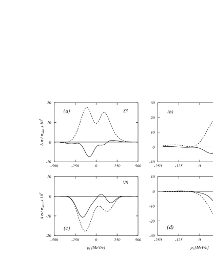
Figure 5: Normalized differences between the correlated and uncorrelated cross sections of Fig. 4. These are the differences between the cross sections divided by the maximum values of the uncorrelated cross sections. The dashed lines represent the two-point diagrams results while the full lines those obtained with the full calculations. The left panels show the perpendicular kinematics results and the right panels the parallel ones.

In order to emphasize the effect of the correlations we present in Fig. 5 the same results in terms of difference between the correlated cross sections and the uncorrelated ones. In order to have a relative measure of the effect we have divided these differences by the maximum values of the uncorrelated cross sections. Henceforth we shall call these results normalized differences.

The effect of the two-point diagrams is rather different for the S3 and V8 calculations. In the former case is positive, the mean field cross section is increased by the correlations, while it is negative in the latter case. It is interesting to notice that the final result is rather similar in both cases as one would expect given the strong similarity of the two correlation functions used.

The effect of the correlations on the individual responses calculated in perpendicular kinematics is shown in Fig. 6. We should first notice that the charge response $W_{L}\equiv W_{0,0}$ and the transverse response $W_{T}\equiv W_{+1,+1}+W_{-1,-1}$ are much larger than the interference responses $W_{TL}\equiv 2Re(W_{-1,0}-W_{0,+1})$ and $W_{TT}\equiv 2Re(W_{+1,-1})$. In the charge response $W_{L}$ the various terms of the correlations behave like the full cross sections, the final results being a lowering of the mean-field response. This is not the case for the $W_{T}$ response, showing an increase of the mean-field results. This effect has been discussed in detail in Ref.[16] where it has been shown that it is related to the absence of the diagram (2.3) of Fig. 2 in the longitudinal response.

In what refers to the interference responses, the behavior of $W_{TL}$ is similar to that of $W_{L}$. In $W_{TT}$ the correlations increases the mean field responses. In this last responses the 3-point diagrams appear to be very sensitive to the input, their contribution is negligible for V8 calculation and noticeable for the S3 ones.

Figure 6: Differences between correlated and uncorrelated response functions in the perpendicular kinematics for the calculations of Fig. 4. The differences have been divided by the maximum value of the uncorrelated responses. The full lines represent the results of the complete calculations and the dashed ones those obtained using the two-point diagrams only.

Figure 7: Normalized differences between correlated and uncorrelated cross sections calculated in perpendicular kinematics for different values of the momentum transfer $q\equiv|{\bf q}|$. As in the previous figures the dashed lines refer to the two-point diagrams calculations while the full lines show the results of the full calculation.

The cross section is obtained by summing the contributions of all the responses. From Eq. (35) one can observe that the $W_{TL}$ responses is added for positive values of $p_{i}$ and subtracted for the negative ones, and this generates the asymmetry in the perpendicular cross sections of Fig. 4.

We have investigated the momentum transfer dependence of the correlation effects by calculating (e,e’p) cross sections in perpendicular kinematics for different values of $|{\bf q}|$. In all the calculations we have fixed the momentum of the emitted nucleon such that $|{\bf p}|=|{\bf q}|$. Results obtained for four different values of $|{\bf q}|$ are shown in Fig. 7 as normalized differences. As in the previous figures the dashed lines show the results obtained by adding to the mean field calculation the two-point diagrams only, while the full lines show the results of the full calculation where also the three-point diagrams have been added. The shape of the lines is slightly modified at different values of $|{\bf q}|$, but the order of magnitude of the effect is almost the same. It is interesting to notice that the cancellation of the two-point diagrams effects produced by the inclusion of the three-point terms generates results rather independent from the correlation function.

Figure 8: Cross sections for the emission of the 1p_3/2 proton in perpendicular kinematics for the S3 and V8 input parameters. The dashed lines show the results obtained adding the two-point diagrams to the uncorrelated terms and the full lines the result of the complete calculation. The uncorrelated results are almost exactly overlapped to the full ones and have not been shown. In the panels $a$ and $b$ we show the cross sections while in the panels $c$ and $d$ the normalized differences between correlated and uncorrelated cross sections.

Figure 9: The same as the previous figure for the emission of the 1s_1/2 proton.

We have also verified the possible changes of the correlation effects depending upon the hole wave function. As an example we show in Figs. 8 and 9 the cross sections, and the normalized differences, obtained for the emission of the 1p_3/2 and 1s_1/2 protons under the same perpendicular kinematics of Fig. 4. While for the 1p_3/2 case the shapes of the cross sections are noticeably similar to those previously shown, the curves obtained for the 1s_1/2 proton are rather different. The small differences in the radial shapes of the two p hole wave functions do not modify sensitively the behavior of the cross section. On the other hand, the big difference in the s wave cross section is due to the different radial shape of the hole wave function. In spite of this the behavior of the correlation effects is analogous in all the cases we have considered. The calculations done with two-point diagrams show noticeable sensitivity to the change of the correlation, while, when the three-point diagrams are added all the results are similar and almost independent of the correlation function.

4.2 Orthogonality and consistency of the input

In the analysis of the (e,e’p) experiments it is a common practice to use a real mean field potential to describe the hole wave function while the particle wave function is described using an optical potential containing also an imaginary part. This procedure, adopted to take into account the final state interaction of the emitted particle with the rest nucleus, produces a non orthogonality between particle and hole single particle wave functions. The effects of this procedure on the (e,e’p) cross section have been thoroughly studied in Ref. [37] where it has been shown that they are negligible for the typical kinematics used in the experiments.

We have investigated the non orthogonality effects when correlations are included in the calculations. In our derivation of the transition matrix elements the orthogonality of the single particle wave functions is essential. On the other hand, since we use central potentials, only the radial parts of the wave functions change, therefore all the angular momentum algebra is still valid. This means that the non orthogonality is present only between single particle wave functions having the same angular momentum but different number of nodes in the radial part.

We have done two calculations where the particle wave functions have been evaluated with a different mean field with respect to the hole wave functions. In the first one the particle mean field was set to zero; therefore the emitted particle wave function was described as a plane wave. This kind of calculation is commonly referred as the Plane Wave Impulse Approximation (PWIA). In the second type of calculation we used the optical potential of Ref. [38] with the parameterization adapted for ¹⁶O in Ref. [35].

Figure 10: Cross sections calculated in perpendicular kinematics under the same conditions of Fig. 4 with different mean field potentials for the particle wave functions. In panels $a$ and $b$ the results obtained in Plane Wave Impulse Approximations are presented. In panels $c$ and $d$ those obtained the optical potential of Schwandt et al. [38]. The meaning of the line is the same as in Fig. 4.

We show in Fig. 10 the cross sections calculated with the S3 and V8 inputs for the same perpendicular kinematics conditions used in Fig. 4. The panels $a$ and $b$ show the PWIA results, while the other two panels those obtained with the optical potential. A comparison with Fig. 4 shows that the PWIA cross sections are larger than the original ones, while the cross sections obtained with the optical potential are smaller. It is interesting to notice that the PWIA results have a minimum for $p_{i}$=0 which is exactly zero, at expected, because in this approximation the cross section is related to the Fourier transform of the hole wave function.

Figure 11: Normalized differences between the cross sections presented in Fig. 10. The meaning of the lines is the same as in Fig. 5.

Figure 12: Normalized differences between cross sections calculated with the same mean field potential but with different correlation functions. In panels $a$ and $b$ the S3 mean field has been used, while in panels $c$ and $d$ the V8 mean field was considered. The S3 and V8 labels indicate the correlation function used. The calculations of the $a$ and $c$ panels have been done in perpendicular kinematics and those of the $b$ and $d$ panels in parallel kinematics. As usual the dashed lines refer to calculations with two-point diagrams while the full lines represent the complete calculations.

In both kinds of calculations the effect of the correlations is very small and to emphasize it we show in Fig. 11 the normalized differences. The behavior of the various terms is similar to that shown in Fig. 5. The results obtained with the two-point terms are rather different when calculated with S3 and V8 inputs. When also the three-point diagrams are included they become similar. Clearly the effects of the non-orthogonality of the basis are negligible on the correlations. We have obtained similar results also in parallel kinematics.

A comparison between the three calculations done in perpendicular kinematics shows that the shapes of the results obtained in PWIA and with the optical potential are rather similar and quite different from the results obtained with the same real potential used for the hole states. This arises because the real part of the Scwhandt potential is quite weak, $-28.359$ MeV, against the about $-50$ MeV of the potential used in our V8 and S3 calculations. The effect of the optical potential is to conserve the PWIA shapes but to lower the values of the cross section. This second effect is obtained because of the presence of the imaginary part of the potential.

We have already stressed that our inputs are taken from microscopic FHNC calculations where, for a given hamiltonian, the energy mean value has been minimized by varying both mean field and correlation function. This consistency of the input is not usually respected in (e,e’p) calculations with short-range correlations, where mean field and correlation functions are taken from different sources.

We have tested the need of relating mean-field and correlation functions by interchanging them in our inputs. This means that we have done calculations using the S3 mean field potential together with the V8 correlation functions, and vice versa. The results of these calculations are shown in Fig. 12 as normalized differences and are compared in each panel with the results of Fig. 5. Also in this figure the need of including three-point diagrams for the reasons already mentioned becomes evident. The final results seems to be rather independent of the mean field used. On the other hand, the quantity shown has been defined to minimize the effects of the mean field and enhance those of the correlations.

4.3 Comparison with other approaches

In this section we shall try to make a comparison between our approach and other models that handle short-range correlations in electron scattering. Depending upon the methodology used to attack the problem we classify these models into two categories. A first kind of calculations [15] uses an approach similar to ours but the evaluation of the diagrams remains restricted to the so-called single pair approximation. This approximation implies that only those two-point diagrams where the knocked out particle is directly connected to the electromagnetic operators are considered. In our classification scheme these are the diagrams (2.1) and (2.2) of Fig. 2, even though the exchange diagram (2.2) is not always considered.

The second category of calculations [10, 14] is based upon the idea of the spectral function [1, 2]. The basic hypothesis is that the nuclear finite state wave function can be separated in terms of emitted particle wave function and spectral function which is related to the overlap between the wave function of the target nucleus and that of the A-1 nucleon system. Spectral functions used in the evaluation of (e,e’p), and also (e,e’2N), cross sections have been calculated in various manners. In some case the Brueckner G-matrix theory has been used [10], in others they have been obtained from variational Monte Carlo calculations [39]. In the work of Ref. [14] the spectral functions have been obtained using the asymptotic properties of the one-body density matrices obtained from microscopic theories. A precise comparison with our approach is rather difficult since the spectral functions include high order correlation terms which we do not consider. What remains, however, is the fact that also this approach considers only those diagrams where the emitted particle is directly connected to the electromagnetic operators. In our approach this could be translated by saying that in addition to the diagrams (2.1) and (2.2), already mentioned, also the diagrams (3.3) and (3.4) are considered.

We have tried to mimic the other approaches by repeating the calculations of Fig. 4 without those diagrams where the particle is not directly connected to the electromagnetic operators. In these calculations the 1/2 and 1/3 terms multiplying the two and three point diagrams respectively have been set to 1, as is done in the literature.

Figure 13: Normalized differences between correlated and uncorrelated cross sections. The full lines represents the complete calculations, the dotted lines have been evaluated by adding to the mean field the contribution of the diagram (2.1) of Fig. 2, the dashed dotted lines, the contribution of the diagrams (2.1) and (2.2) and the dashed lines, the diagrams (2.1), (2.2), (3.4) and (3.5).

The results of these calculations are presented in Fig. 13 as normalized differences. The full lines show the results of the complete calculations, those of Fig. 4. The dotted lines have been obtained by using the diagram (2.1) only, the dashed dotted lines have been obtained by adding also the diagram (2.2) and the dashed lines by adding the diagrams (3.3) and (3.4).

The inclusion of the diagrams (3.3) and (3.4) changes radically the effect of the correlations, modifying shapes and signs. The final result in the case of S3 is rather similar to that of the complete calculation, but for the V8 input there is a noticeable difference. This instability of these results shows, in a clear manner, the need of including all the terms of the expansion.

4.4 Comparison with experimental data

In this section we compare the results of our calculations with some experimental data available on ¹⁶O. In the literature these data are presented in terms of a reduced cross section obtained by dividing the cross section by the electron-nucleon cross section and the kinematic factor $K$ of Eq. (1). In our calculations we have used the electron-nucleon $\sigma_{cc1}$ cross section of Ref. [40].

In Fig. 14 we make the comparison with the 1p_1/2 proton emission data of Ref. [34] measured in perpendicular kinematics. The full lines represent the complete calculations of Fig. 4, where all the diagrams are considered and the same mean-field potential for both particles and hole has been used. In the panels $a$ and $b$ the results for the S3 and V8 inputs are shown respectively. In the panels $c$ and $d$ the same curves have been multiplied by reduction factors to improve the agreement with the experimental data. These factors are 0.58 for the S3 result and 0.5 for the V8 one. Even after quenching the curves the agreement with the data is rather poor.

Figure 14: Reduced cross section compared with the experimental data of Saclay [34]. The full lines have been obtained from the complete calculations of Fig. 4 in perpendicular kinematics. The dashed lines have been calculated with the optical potential of Ref. [38]. In panels $c$ and $d$ the curves of the upper panels have been multiplied by reduction factors to reproduce the data (see text).

The dashed lines of the figure have been obtained by changing the particle mean field with the optical potential of Schwand et al. [38], in the parameterization of Ref. [35]. Also in this case a quenching of the curves is necessary, and the final results, shown in the two lower panels, have been obtained multiplying by 0.58 and 0.5 the S3 and V8 results respectively. The dashed curves show a better agreement with the experimental data.

Figure 15: Reduced cross sections compared with the experimental data of Nikhef [35]. The full lines have been obtained from the complete calculations of Fig. 4 in parallel kinematics. The dashed lines have been calculated with the optical potential of Ref. [38]. In panels $c$ and $d$ the curves of the upper panels have been multiplied by a common reduction factors of 0.8.

An analogous situation is found in Fig. 15 where the comparison is done with the data of Ref. [35], again for the emission of the 1p_1/2 proton but measured in parallel kinematics. The meaning of the curves is the same of the previous figure, and in this case we used for all the curves the same quenching factor of 0.8.

The results presented in Figs. 14 and 15 clearly show that the fully consistent calculations are unable to reproduce the data. Not only in terms of their magnitude, but the obtained results are qualitative different with respect to the data distribution. The mean fields fixed by the minimization process in Ref. [21] and [22] are too strong to describe properly the motion of the emitted particle in the continuum as we have already observed. The shift of the minimum of the reduced response with respect to $p_{i}=0$ in parallel kinematics is an effect produced by the distortion potential.

Figure 16: Response functions compared with the experimental data of Ref. [41]. Our calculations have been done with the S3 input and using the optical potential of Ref. [38]. The full lines show the results of the complete calculations, the dashed ones those obtained with the two-point diagrams, and the dotted lines (overlapped to the full ones), the mean-filed results. The panel labelled $W_{L}$ shows actually $W_{L}+\frac{1}{2}\frac{{\bf q}^{2}}{{\bf q}^{2}-\omega^{2}}W_{TT}$. The contribution of $W_{TT}$ is in any case small. The response $W_{TL}$ is multiplied by $1/\sqrt{2}$ in order to agree with the response experimentally separated. All the curves have been multiplied by a 0.7 factor.

In Fig. 16 we compare the results of our calculations with the empirical values of the electromagnetic responses given in Ref. [41]. These calculations have been done with the S3 input and using the Scwhandt et al. optical potential [38]. The meaning of the various lines is that of Fig. 4: full lines show the complete calculations and dashed lines have been obtained by adding the two-points diagrams to the mean-field terms. We do not draw the mean-field results because they are almost overlapped with the full ones. All the lines have been multiplied by a reduction factor of 0.7. The effect of the short range correlations is very small. One can clearly identify the increasing of the responses produced by the inclusion of only the two-point diagrams, but the final results are essentially back to mean-field result. The calculation done with the V8 input produces analogous results, with the obvious difference in the two-point calculations. The same data have been studied in Ref. [42] where it has been shown that the effects of the Meson Exchange Current are larger than those we find for the short-range correlations.

5 Summary and conclusions

In this work we have studied the effects of short-range correlations on the one-nucleon emission processes induced by electromagnetic probes. The description of these processes has been done by using a nuclear model that considers all the linked diagrams containing a single correlation line. This implies that in addition to the two-point diagrams, commonly considered in the literature, also three-point diagrams should be included in order to maintain the proper normalization of the many-body wave function.

The calculations have been done using single particle wave functions and correlations taken from microscopic FHNC calculations [21, 22]. We have considered only the scalar term of the correlation. We have calculated the ¹⁶O (e,e’p) ¹⁵N reaction for the perpendicular and parallel kinematics of the Saclay and Nikhef experiments of Refs. [34] and [35].

In the kinematic conditions investigated, the effects of the short-range correlations are extremely small as compared to the mean-field results. They are within the accuracy of the experimental data and the uncertainty in the theoretical inputs.

The two correlation functions used in our calculations are rather similar, and therefore we expect them to produce similar effects on the mean–field results. This does not happens if only two-point diagrams are included. The S3 increases the mean-field responses, and cross sections, while the V8 lowers their values. The effects of the correlations become similar when the three-point diagrams are included. The detailed study of the separated responses shows that the three-point diagrams reduce the effect produced by the two-point diagrams alone, whatever they are. This fact is a consequence of the need of the three-point diagrams to ensure the proper normalization of the wave function. This result is almost independent of the momentum transfer or hole wave function.

We have been concerned about the consistency of the input, and we have calculated cross sections with different mean fields describing the emitted particle, and we have also interchanged correlation functions and mean field in our inputs. We did not find significant changes on the effects of the correlations, saying that these effects are rather independent of the chosen mean field.

We have tried to compare our short-range correlation model with other approaches one finds in the literature. In these approaches only those diagrams where the emitted particle is directly connected to the one-body electromagnetic operator are considered. We have done calculations where only these diagrams have been considered, and we found a strong dependence of the results on the number of diagrams included, showing big instabilities to small changes of the input. The situation is rather complicated by the fact that in these approaches the particle wave function is usually described as moving in an optical potential. Therefore it is not clear whether the diagrams we have calculated explicitly are effectively considered by the optical potential.

The comparison with the experimental data of Refs. [34, 35, 41], shows that the short-range correlation effects do not significantly improve the agreement with the data. In this respect various problems remain open, such as the physical origin of the required quenching or the reason why the parameters of the optical potential are so different from those describing the hole states. The investigation of these problems is beyond the scope of the present article.

Finally we would like to discuss some of the limitations of our calculations related to the hypotheses and the approximations of our model. One of these limitations is due to the fact that we consider only those diagrams containing a single correlation function. Clearly higher order terms could be important. We have already mentioned that the test of the validity of our model was done in Ref. [20] for the inclusive nuclear matter charge response. The excellent agreement between our results and those obtained considering an infinite set of diagrams, give us confidence about our approximation, and we trust its validity also in the case of finite nuclear systems and for the one-body current operators. It would be interesting, in any case, to make other tests on it.

Another limitation of our approach is related to the use of correlation functions of purely Jastrow type. Recent calculations show that the tensor correlations on two-nucleon emission processes [15, 43] produce effect comparable, or even larger, than those induced by the scalar correlations. However, these calculations have been done in the single pair approximation, and we have shown how dangerous is to rely on such an approximation which can produce large effects since the three-point counter terms are not present. On the other hand, we know from microscopic calculations [44] that the tensor correlations are essential to bind nuclei. They are also important, together with Meson Exchange Currents, in the nuclear matter transverse quasi-elastic response [45] and they are necessary to obtain a proper description of the electromagnetic responses of few-body systems [46]. The possible effect of the tensor correlations on nuclear responses is an open problem which should be investigated.

Last, but not least, our model does not take into account those processes beyond the mean-field description of the nucleus falling under the generic name of long-range correlations. These correlations are related to the coupling between the single particle dynamics and the collective excitation modes of the nucleus. Their effects on (e,e’p) processes have been considered in a nuclear matter approach [10], but they do not seem to be relevant. However, one should consider that collective surface vibrations are not present in nuclear matter calculations, and they can be extremely important in finite nuclear systems, as an investigation on the charge density distribution differences of heavy isotones has recently pointed out [47].

Acknowledgments
We thank C. Giusti for useful discussions and M. Leuschner for sending us the experimental data. One of us, S.R.M., thanks the Italian Foreigner Ministry for the financial support during his stay in Lecce. This work has been partially supported by the agreement INFN-CICYT, by the DGES (PB98-1367), by the Junta de Andalucía (FQM225) and by the MURST trough the PRIN: Fisica teorica del nucleo atomico e dei sistemi a molticorpi.

References

- [1] S. Frullani and J. Mougey, Adv. Nucl. Phys, 14 (1984),1.
- [2] S. Boffi, C. Giusti, F.D. Pacati and M. Radici, Electromagnetic Response of Atomic Nuclei (Clarendon Press, Oxford, 1996).
- [3] P.K.A. de Witt Huberts, J. Phys. G, 16 (1990), 507.
- [4] G.J. Wagner, in Nuclear Structure at High Spin, Excitation, and Momentum Transfer, H. Mann ed., AIP Conf. Proc. No 142, (AIP, New York, 1982), p. 220.
- [5] J.M. Udías, P. Sarriguren, E. Moya de Guerra, E. Garrido and J.A. Caballero, Phys. Rev C 48 (1993), 2731.
- [6] G. van der Steenhoven, H.P. Blok, J.F.J. van der Brand, T. de Forest Jr., J.W.A. den Herder, E. Jans, P.H.M. Keizer, L. Lapikás, P.J. Mulders, E.N.M. Quint, P.K.A. de Witt Huberts, J. Mougey, S. Boffi, C. Giusti and F.D. Pacati, Phys. Rev. Lett. 57 (1986), 182; G. van der Steenhoven, A.M. van den Berg, H.P. Blok, S. Boffi, J.F.J. van der Brand, R. Ent, T. de Forest Jr., C. Giusti, J.W.A. den Herder, E. Jans, G.J. Kramer, J.B.J.M. Lanen, L. Lapikás, J. Mougey, P.J. Mulders, F.D. Pacati, E.N.M. Quint, and P.K.A. de Witt Huberts, Phys. Rev. Lett. 58 (1987), 1727.
- [7] V.R. Pandharipande, C.N. Papanicolas and J. Wambach, Phys. Rev. Lett.53 (1984), 1133.
- [8] A. Ramos, A. Polls and W.H. Dickhoff, Nucl. Phys. A 503 (1989), 1.
- [9] O. Benhar, A. Fabrocini and S. Fantoni, Nucl. Phys. A 505 (1989), 267.
- [10] K. Amir-Azimi-Nili, J.M. Udias, H. Müther, L.D. Skouras and A. Polls, Nucl. Phys. A 625 (1997), 633. A. Polls, M. Radici, S. Boffi, W.H. Dickhoff and H. Müther, Phys. Rev. C 55 (1997), 810.
- [11] A. Fabrocini and G. Co’, Phys. Rev. C 63 (2001) 044319.
- [12] C. Giusti and F.D. Pacati, Nucl. Phys. A 571 (1994), 694.
- [13] J. Ryckebusch, V. Van der Sluys, K. Heyde and M. Waroquier, Phys. Lett. B 350 (1995), 1; J. Ryckebusch, V. Van der Sluys, K. Heyde, H. Holvoet, W. Van Nespen and M. Waroquier, Nucl. Phys. A 624 (1997), 581.
- [14] M.K. Gaidarov, K.A. Pavlova, A.N. Antonov, M.V. Stoitsov, S.S. Dimitrova, M.V Ivanov and C. Giusti, Phys. Rev. C 61 (2000), 014306.
- [15] S. Janssen, J. Ryckebusch, W. Van Nespen and D. Debruyne, Nucl. Phys. A 672 (2000), 285; J. Ryckebusch, S. Janssen, W. Van Nespen and D. Debruyne, Phys. Rev. C 61 (2000), 021603.
- [16] G. Co’ and A.M. Lallena, Ann. Phys. (NY) 287 (2001) 101.
- [17] J.W. Clark, Prog. Part. and Nucl. Phys., 2 (1979) 89; S. Rosati, in From nuclei to particles, Proc. Int. School E. Fermi, course LXXIX, ed. A. Molinari (North Holland, Amsterdam, 1982), p73.
- [18] G. Co’, Nuov. Cim. A 108 (1995), 623.
- [19] F. Arias de Saavedra, G. Co’ and M.M. Renis, Phys. Rev. C 55 (1997), 673.
- [20] J.E. Amaro, A.M. Lallena, G. Co’ and A. Fabrocini, Phys. Rev. C 57 (1998), 3473.
- [21] F. Arias de Saavedra, G. Co’, A. Fabrocini and S. Fantoni, Nucl. Phys. A 605 (1996), 359.
- [22] A. Fabrocini, F. Arias de Saavedra and G. Co’, Phys. Rev. C 61 (2000), 044302.
- [23] J.D. Bjorken and S.D. Drell, Relativistic Quantum Mechanics, (McGraw Hill, New York, 1964).
- [24] T. de Forest Jr., Ann. Phys. (NY) 45 (1967), 365; A.E. Dieperink and T. de Forest Jr., Ann. Rev. Nucl. Sc. 25 (1975), 1; W.E. Kleppinger and J.D. Walecka, Ann. Phys. (NY) 146 (1983), 349.
- [25] G. Co’ and S. Krewald, Nucl. Phys. A 433 (1985), 392.
- [26] G. Co’, A.M. Lallena and T.W. Donnelly, Nucl. Phys. A 469 (1987), 684.
- [27] G. Hoehler, E. Pietarinen, I. Sabba-Stefabescu, F. Borkowski, G.G. Simon, V.H. Walther and R.D. Wendling, Nucl. Phys. B 114 (1976), 505.
- [28] A.R. Edmonds, Angular momentum in quantum mechanics, (Princeton University Press, Princeton, 1957).
- [29] S. Fantoni and V. R. Pandharipande, Nucl. Phys. A 473 (1987), 234.
- [30] C. Giusti and F.D. Pacati, Nucl. Phys. A 473 (1987), 717; Y. Jin, D.S. Onley and L.W. Wright, Phys. Rev C 45 (1992), 1311; V. Van der Sluys, K. Heyde, J. Ryckebusch and M. Waroquier, Phys. Rev C 55 (1997), 1982.
- [31] I.R. Afnan and Y.C. Tang, Phys. Rev 175 (1968), 1337.
- [32] R.B. Wiringa, V.G.J. Stoks and R. Schiavilla, Phys. Rev. C 51 (1995), 38.
- [33] B.S. Pudliner, V.R. Pandharipande, J. Carlson, S. C. Pieper and R. B. Wiringa, Phys. Rev. C 56 (1997), 1720; R. Schiavilla, V.R. Pandharipande and R.B. Wiringa, Nucl. Phys. A 449 (1986), 219.
- [34] M. Bernheim, A. Bussière, J. Mougey, D. Royer, D. Tarnowsky, S. Turk-Chièze, S. Frullani, S. Boffi, C. Giusti, F.D. Pacati, G.P. Capitani, E. De Sanctis and G.W. Wagner, Nucl. Phys. A 375 (1982), 381.
- [35] M. Leuschner, J. Calarco, F.W. Hersman, E. Jans, G.J. Kramer,L. Lapikás, G. van der Steenhoven, P.K. de Witt Huberts, H.P. Blok, N. Kalantar-Nayestanaki, and J. Friedrich, Phys. Rev. C 49 (1994), 955.
- [36] S.R. Mokhtar, G. Co’ and A.M. Lallena, Phys. Rev. C 62 (2000) 067304.
- [37] S. Boffi, F. Cannata, F. Capuzzi, C. Giusti and F.D. Pacati, Nucl. Phys. A 379 (1982), 509.
- [38] P. Schwandt, H.O. Meyer, W.W. Jacobs, A.D. Bacher, S.E. Vigdor, M.D. Kaitchuck and T.R. Donoghue, Phys. Rev. C 26 (1982), 55.
- [39] L. Lapikás, J. Wesseling and R.B. Wiringa, Phys. Rev. Lett. 82 (1999), 4404.
- [40] T. de Forest Jr., Nucl. Phys. A 392 (1983), 232.
- [41] C.M. Spaltro, H.P. Blok, E. Jans, L. Lapikás, M. van der Schaar, G. van der Steenhoven and P.K.A de Witt Huberts, Phys. Rev. C 48 (1993), 2385.
- [42] J.E. Amaro, A.M. Lallena and J.A. Caballero, Phys. Rev. C 60 (1999), 014602.
- [43] C. Giusti, H. Müther, F.D. Pacati and M. Stauf, Phys. Rev. C 60 (1999), 054608.
- [44] A. Fabrocini, F. Arias de Saavedra, G. Co’ and P. Folgarait, Phys. Rev. C 57 (1998), 1668.
- [45] A. Fabrocini, Phys. Rev. C 55 (1997), 338.
- [46] J. Carlson and R. Schiavilla, Rev. Mod. Phys. 70 (1998), 743.
- [47] M. Anguiano and G. Co’, preprint, Lecce (2001).