Particle number projection with effective forces.

Abstract

The particle number projection method is formulated for density dependent forces and in particular for the finite range Gogny force. Detailed formula for the projected energy and its gradient are provided. The problems arising from the neglection of any exchange term, which may lead to divergences, are thoroughly discussed and the possible inaccuracies estimated. Numerical results for the projection after variation method are shown for the nucleus ¹⁶⁴Er and for the projection before variation approach for the nuclei ^48,50Cr. We also confirm the Coulomb antipairing effect found in mean field theories.

, , ,

1 Introduction

The simplest approach to the many-body system is the mean–field approximation (MFA). The most powerful MFA is the Hartree–Fock–Bogoliubov (HFB) theory, where particle-hole and particle-particle correlations are taken into account at the same foot. The success of this simple approach is based on the large variational Hilbert space generated by symmetry breaking wave functions. For an atomic nucleus and in the most general HFB approach as many symmetries as possible, in particular the rotational invariance and the particle number symmetries are broken. In these approaches the quantum numbers are only conserved on the average, a semiclassical approach to the full quantum requirement to the wave function of being an eigenstate of the symmetry operators. It is well known [1] that the plain HFB approach works well in the case of a strongly correlated regime and with a large number of nucleons participating in the symmetry breaking process. In the case of the rotational invariance, the ideal situation is represented by a strongly deformed heavy nucleus where a large number of nucleons contribute to the collective phenomenon of deformation. In the case of the particle number symmetry, in which we are interested in this paper, the situation is far from being satisfactory because only a few pairs of nucleons ( four to five) in the vicinity of the Fermi surface are thought to cause the phenomenon of nuclear superfluidity. Thus, it is well known that the treatment of pairing correlations in the mean field approach produces an unrealistic transition from the superfluid to the normal phase along the yrast band, not expected in a finite system. In order to get an improved description of the nucleus it is clear that one has to go beyond the mean field approximation to include correlations. This task can be achieved in a simple and effective way within the particle number projection (PNP) [2] formalism, another possibility is to build correlations by the Random-Phase-Approximation (RPA) [3]. The latter is, however, from the applications point of view, very limited, since the required calculation of the ground state correlations can be performed only for very simple models and/or separable interactions. Concerning this point one has to keep in mind that not only the RPA but also other sophisticated theories have been developed only in simple models or with separable forces. Thus the first calculation with exact particle number projection before the variation was done about twenty years ago [4] with the pairing plus quadrupole Hamiltonian and the Baranger-Kumar configuration space.

In the last years in an attempt to achieve some progress in calculations with effective forces and large configuration spaces, the Lipkin Nogami method [5] has experienced a revival. The great advantage of the Lipkin Nogami method is that corrects, in an approximate way, for the zero point energy associated with the breakdown of the particle number symmetry at the mean field level, i.e. the calculations do not get much involved as compared to the full HFB ones. Some applications of this method with effective forces have been done with the Skyrme force [6, 7], the Gogny force[8] and the relativistic mean field approach [9]. The Lipkin Nogami method on the other hand is just a recipe and cannot be obtained from a variational principle. It is therefore desirable to develop an exact particle number projection which can be applied to effective forces. The purpose of this paper is to develop an exact particle number projection before (and after) the variation for density dependent forces and in particular for the Gogny force. As we shall see, the exchange terms play an important role in PNP, in fact the neglection of any exchange term may lead to divergences. As it is well known, in general, a zero range force is unable to provide good pairing properties. As a matter of fact, normally the pairing terms of the force are neglected in order to get reasonable Hartree Fock results. To perform HFB calculations a pairing force has been usually added ad hoc. The finite range of the density dependent Gogny force, on the other hand, provides good pairing properties without neglection of any exchange term. In fact, the force was designed with this intention[10] and this property makes the Gogny force one of the few effective density dependent forces for which particle number projection is feasible without problem due to divergences. All the Skyrme parametrizations (with the few exceptions of those which provide reasonable pairing correlations) and all relativistic mean field approaches may give in general divergent contributions to the projected energy.

In section 2, we introduce the particle number projection method for non-separable density dependent forces. In section 3 we present the formalism for the density dependent part of the interaction and discuss some alternative prescriptions to this dependence. The gradient of the projected energy to be implemented in the calculations is developed in section 4. In section 5, we present results for the projection after variation (PAV) method for the nucleus ¹⁶⁴Er and discuss the problems associated with the divergent terms. Results for the variation after projection (VAP) method for the nuclei ^48,50Cr are discussed in section 6.

2 Particle Number Projected Hartree–Fock–Bogoliubov Theory.

The Particle Number Projected Hartree–Fock–Bogoliubov theory is the simplest symmetry conserving mean field approach which takes into account particle-particle correlations. This theory has been derived in the past for non-density dependent interactions and a detailed formulation has only been given for separable forces like the Pairing Plus Quadrupole model [4]. In order to generalize this theory to non-separable and density dependent forces, like the Gogny or the Skyrme force, and to introduce the pertinent notation we shall also summarize the known formulation.

Let $|\Phi\rangle$ be a product wave function of the HFB type, i.e, the vacuum to the quasiparticle operators given by the Bogoliubov transformation

$${\alpha}_{\mu}=\sum_{k}U^{*}_{k\mu}c_{k}+V^{*}_{k\mu}c_{k}^{\dagger},$$ (1)

where $(c_{k},c_{k}^{\dagger})$ are the particle annihilation and creation operators (usually in the Harmonic Oscillator basis). This transformation does not conserve the particle number symmetry and the wave function $|\Phi\rangle$ is not an eigenstate of the particle number operator $\hat{N}$. One can generate, however, out of $|\Phi\rangle$, an eigenstate, $|\Psi_{N}\rangle$, of $\hat{N}$ by the well known projection technique [1]

$$|{\Psi}_{N}\rangle={\hat{P}}^{N}|\Phi\rangle=\frac{1}{2\pi}\int_{0}^{2\pi}d{\varphi}\,e^{i\varphi(\hat{N}-N)}\,|\Phi\rangle,$$ (2)

where the integration interval can be reduced to $[0,\pi]$ whenever the intrinsic wave function has a well defined “number parity” [1] quantum number. Furthermore, the integral can be discretized in a sum using the Fomenko expansion [11]

$${{\hat{P}}_{L}}^{N}=\frac{1}{L}\sum_{l=1}^{L}e^{i{\varphi}_{l}(\hat{N}-N)},\,\,\,\,\,\,\,\,{\varphi}_{l}=\frac{\pi}{L}l,$$ (3)

where $L$ is the number of points used in the calculations, for $L\rightarrow\infty$ one gets the exact solution, usually $L=8$ is used in the calculations. $P^{N}$ projects only on one system of particles, in the general case, however, one has to perform a double projection, for the number of neutrons and protons. In this case the projected matrix element of any operator $\hat{O}$, such that $[\hat{O},\hat{N}]=0$, is given by [4]

$$O^{P}=\frac{\langle\Phi|\hat{O}\hat{P}^{N_{\pi}}\hat{P}^{N_{\nu}}|\Phi\rangle}{\langle\Phi|\hat{P}^{N_{\pi}}\hat{P}^{N_{\nu}}\ \Phi\rangle}=\sum_{l_{\pi}=1}^{L}\sum_{l_{\nu}=1}^{L}{\displaystyle y_{l_{\pi}}y_{l_{\nu}}}O({\varphi}_{\pi},{\varphi}_{\nu}),$$ (4)

where we have introduced

$${\displaystyle y_{l_{\tau}}}=\frac{\langle{\Phi}_{\tau}|e^{i{\varphi}_{l_{\tau}}({\hat{N}}_{\tau}-N_{\tau})}|{\Phi}_{\tau}\rangle}{\displaystyle\sum_{l_{\tau}=1}^{L}\langle{\Phi}_{\tau}|e^{i{\varphi}_{l_{\tau}}({\hat{N}}_{\tau}-N_{\tau})}|{\Phi}_{\tau}\rangle},$$ (5)

and the $\hat{O}$-operator overlap

$$O({\varphi}_{\pi},{\varphi}_{\nu})=\frac{\langle{\Phi}|\hat{O}e^{i{\varphi}_{l_{\pi}}{\hat{N}}_{\pi}}e^{i{\varphi}_{l_{\nu}}{\hat{N}}_{\nu}}|{\Phi}\rangle}{\langle{\Phi}|e^{i{\varphi}_{l_{\pi}}{\hat{N}}_{\pi}}e^{i{\varphi}_{l_{\nu}}{\hat{N}}_{\nu}}|{\Phi}\rangle},$$ (6)

with $|{\Phi}\rangle=|{\Phi}_{\pi}\rangle|{\Phi}_{\nu}\rangle$. Another useful quantity is the norm overlap, which is given by

$$x_{l_{\tau}}=\langle{\Phi}_{\tau}|e^{i{\varphi}_{l_{\tau}}({\hat{N}}_{\tau}-N_{\tau})}|{\Phi}_{\tau}\rangle,$$ (7)

clearly, ${y_{l_{\tau}}}$ and $x_{l_{\tau}}$ are related by ${\displaystyle y_{l_{\tau}}}={\displaystyle y^{\tau}_{0}}x_{l_{\tau}}$, with $y^{\tau}_{0}=(\sum_{l_{\tau}=1}^{L}x_{l_{\tau}})^{-1}$.

As it will be illustrated for the Hamiltonian operator, any operator overlap can be calculated using the generalized Wick theorem [12]. This theorem allows to express matrix elements of the form $\langle\Phi|\hat{O}|\tilde{\Phi}\rangle$, exactly in the same way as the ordinary Wick theorem, as the sum of all possible contracted products, where $|{\Phi}\rangle$ and $|\tilde{\Phi}\rangle$ are quasiparticle vacua. Thus, in particular

$$\langle\Phi|{c}^{\dagger}_{k_{1}}{c}^{\dagger}_{k_{2}}c_{k_{4}}c_{k_{3}} |\tilde{\Phi}\rangle=\langle\Phi|\tilde{\Phi}\rangle^{-1}\left[\langle\Phi|{c}^{\dagger}_{k_{1}}c_{k_{3}}|\tilde{\Phi}\rangle\langle\Phi|{c}^{\dagger}_{k_{2}}c_{k_{4}}|\tilde{\Phi}\rangle\right.$$ (8)

$$-\left.\langle\Phi|{c}^{\dagger}_{k_{1}}c_{k_{4}}|\tilde{\Phi}\rangle\langle\Phi|{c}^{\dagger}_{k_{2}}c_{k_{3}}|\tilde{\Phi}\rangle+\langle\Phi|{c}^{\dagger}_{k_{1}}{c}^{\dagger}_{k_{2}}|\tilde{\Phi}\rangle\langle\Phi|c_{k_{4}}c_{k_{3}}|\tilde{\Phi}\rangle\right]$$

Looking at eq. (4) we see that this theorem allows to express projected expectation values in terms of mean field matrix elements. In eq. (8) the first term is the Hartree term, the second one the Fock term and the last one the Bogoliubov term. ¿From this expression we see that problems may appear when $\langle\Phi|\tilde{\Phi}\rangle\approx 0$. This point will be discussed later on and its consequences for the effective force will be analyzed in Appendix B. For the PNP method, the basic building blocks of Wick’s theorem are the $\varphi$-dependent generalized density matrix and pairing tensors

$${\rho}_{kk^{\prime}}(\varphi) = \frac{\langle\Phi|{c^{\dagger}_{k^{\prime}}}c_{k}|\tilde{\Phi}\rangle}{\langle\Phi|\tilde{\Phi}\rangle}=\frac{\langle\Phi|{c^{\dagger}_{k^{\prime}}}c_{k}e^{i\varphi\hat{N}}|\Phi\rangle}{\langle\Phi|e^{i\varphi\hat{N}}|\Phi\rangle}={\left({\mathcal{V}}^{*}(\varphi)V^{T}\right)}_{kk^{\prime}}$$ (9)

$${\kappa}_{kk^{\prime}}^{10}(\varphi) = \frac{\langle\Phi|c_{k^{\prime}}c_{k}|\tilde{\Phi}\rangle}{\langle\Phi|\tilde{\Phi}\rangle}=\frac{\langle\Phi|c_{k^{\prime}}c_{k}e^{i\varphi\hat{N}}|\Phi\rangle}{\langle\Phi|e^{i\varphi\hat{N}}|\Phi\rangle}={\left({\mathcal{V}}^{*}(\varphi)U^{T}\right)}_{kk^{\prime}}$$ (10)

$${\kappa}_{kk^{\prime}}^{01}(\varphi) = \frac{\langle\Phi|c_{k}^{\dagger}c_{k^{\prime}}^{\dagger}|\tilde{\Phi}\rangle}{\langle\Phi|\tilde{\Phi}\rangle}=\frac{\langle\Phi|c_{k}^{\dagger}c_{k^{\prime}}^{\dagger}e^{i\varphi\hat{N}}|\Phi\rangle}{\langle\Phi|\ e^{i\varphi\hat{N}}|\Phi\rangle}={\left(V{\mathcal{U}}^{\dagger}(\varphi)\right)}_{kk^{\prime}}$$ (11)

where we have used the notation $|\tilde{\Phi}>=e^{i\varphi\hat{N}}|\Phi>$, the indices $(k,k^{\prime})$ belonging to the same isospin channel $\tau$. The matrices ${\mathcal{U}}(\varphi)$ and ${\mathcal{V}}(\varphi)$ are related to $U$ and $V$ of eq. (1) by

$${\mathcal{U}}(\varphi)\,=\,U\,+\,V^{*}{{\mathcal{X}}(\varphi)}^{*}\;\;\;\;\;\;\;\;{\mathcal{V}}(\varphi)\,=\,V\,+\,U^{*}{{\mathcal{X}}(\varphi)}^{*},$$ (12)

and the contraction ${\mathcal{X}}(\varphi)$ is given by

$${\mathcal{X}}_{\mu\nu}(\varphi)=\frac{\langle\Phi|{\alpha}_{\nu}{\alpha}_{\mu}|\tilde{\Phi}\rangle}{\langle\Phi|\tilde{\Phi}\rangle}={\left(T_{21}^{*}(\varphi)T_{22}^{-1}(\varphi)\right)}_{\mu\nu},$$ (13)

here again the indices ${\mu,\nu}$ belong to the same isospin channel and

$$T_{22}\,({\varphi}) = \cos({\varphi})\cdot{\mbox{\Large\bf$1\!\!1$}}\,-\,i\sin({\varphi})\cdot{\hat{N}}^{11}$$ (14)

$$T_{21}(\varphi)\, = \,-\,i\sin({\varphi})\cdot{\hat{N}}^{20}$$ (15)

with ${N}^{11}=U^{\dagger}U-V^{\dagger}V$ and ${N}^{20}=U^{\dagger}V^{*}-V^{\dagger}U^{*}$. The matrices ${N}^{11}$ and ${N}^{20}$ represent the number operator in the quasiparticle basis of eq.(1).

The nuclear Hamiltonian can be written as

$$\hat{H} = T+\hat{V}_{DI}+\hat{V}_{DD}$$ (16)

$$= \sum_{k_{1}k_{2}}t_{k_{1}k_{2}}{c}^{\dagger}_{k_{1}}c_{k_{2}}\,+\,\frac{1}{4}\sum_{k_{1}k_{2}k_{3}k_{4}}{\bar{v}}_{k_{1}k_{2}k_{3}k_{4}}{c}^{\dagger}_{k_{1}}{c}^{\dagger}_{k_{2}}c_{k_{4}}c_{k_{3}}+\hat{V}_{DD}$$

where the density independent part, $\hat{V}_{DI}$, represents the nuclear interaction (Coulomb included) with the exception of a possible density-dependent term (the well known density dependent term of the Skyrme and Gogny forces) which is represented by $\hat{V}_{DD}$. In our case $\hat{V}_{DD}$ is given by the last term of eq. (60).

2.1 Particle Number Projected Energy for the non-density dependent parts of the interaction.

With the definitions above we can formulate the particle number projected theory for non–separable interactions, like the Gogny force (Appendix A), in a similar way as in the mean field approximation. Using eq. (4) and the generalized Wick theorem, the density independent part of the projected energy is given by

$$E^{P}_{DI} = \sum_{l_{\pi}=1}^{L}\sum_{l_{\nu}=1}^{L}y_{l_{\pi}}y_{l_{\nu}}\cdot Tr\biggl{\{}t\left({\rho}({\varphi}_{l_{\pi}})+{\rho}({\varphi}_{l_{\nu}})\right)$$ (17)

$$+ \frac{\,1\,}{2}\Bigl{(}{\Gamma}^{\pi\pi}({\varphi}_{l_{\pi}})\rho({\varphi}_{l_{\pi}})+{\Gamma}^{\pi\nu}({\varphi}_{l_{\nu}})\rho({\varphi}_{l_{\pi}})+{\Gamma}^{\nu\pi}({\varphi}_{l_{\pi}})\rho({\varphi}_{l_{\nu}})$$

$$+ {\Gamma}^{\nu\nu}({\varphi}_{l_{\nu}})\rho({\varphi}_{l_{\nu}})-{\Delta}^{10,\pi}({\varphi}_{l_{\pi}}){\kappa}^{01}({\varphi}_{l_{\pi}})-{\Delta}^{10,\nu}({\varphi}_{l_{\nu}}){\kappa}^{01}({\varphi}_{l_{\nu}})\Bigr{)}\biggr{\}}\,,$$

where the traces run over the configuration space, here assumed to be the same for protons and neutrons, and

$${\Gamma}^{\tau{\tau}^{\prime}}_{k_{1}k_{3}}({\varphi}_{l_{{\tau}^{\prime}}}) = \sum_{k_{2}k_{4}}{\bar{v}}_{k_{1}k_{2}k_{3}k_{4}}{\rho}_{k_{4}k_{2}}({\varphi}_{l_{{\tau}^{\prime}}}),$$ (18)

$${\Delta}^{10,\tau}_{k_{1}k_{2}}(\varphi_{\tau}) = \frac{1}{2}\sum_{k_{3}k_{4}}{\bar{v}}_{k_{1}k_{2}k_{3}k_{4}}{\kappa}^{10}_{k_{3}k_{4}}(\varphi_{\tau}).$$ (19)

In ${\Gamma}^{\tau{\tau}^{\prime}}$ the indices $({k_{1},k_{3}})$ belong to the isospin $\tau$ and $({k_{2},k_{4}})$ to $\tau^{\prime}$, in ${\Delta}^{10,\tau}$ all indices belong to the isospin $\tau$ . Since $\sum_{l_{\tau}=1}^{L}y_{l_{\tau}}=1$, we can write the proton or neutron projected density as

$${\rho}^{P\tau}_{k,k^{\prime}}=\frac{\langle\Phi|{c_{k^{\prime}}}^{\dagger}c_{k}\hat{P}^{N_{\tau}}|\Phi\rangle}{\langle\Phi|\hat{P}^{N_{\tau}}|\Phi\rangle}=\sum_{l_{\tau}=1}^{L}y_{l_{\tau}}{\rho}^{\tau}_{k,k^{\prime}}({\varphi}_{l_{\tau}})\,,$$ (20)

with $(k,k^{\prime})$ belonging to the isospin $\tau$, and the projected energy as

$$E^{P}_{DI} = Tr\Biggl{\{}\Bigl{(}t^{\pi}+\frac{\,1\,}{2}{\Gamma}^{\pi,P\nu}\Bigr{)}{\rho}^{P\pi}+\Bigl{(}t^{\nu}+\frac{\,1\,}{2}{\Gamma}^{\nu,P\pi}\Bigr{)}{\rho}^{P\nu}+$$ (21)

$$+ \frac{\,1\,}{2}\,\sum_{\tau}\sum_{l_{\tau}=1}^{L}y_{l_{\tau}}\Bigl{(}{\Gamma}^{\tau\tau}({\varphi}_{l_{\tau}})\rho({\varphi}_{l_{\tau}})-{\Delta}^{10,\tau}({\varphi}_{l_{\tau}}){\kappa}^{01}({\varphi}_{l_{\tau}})\Bigr{)}\Biggr{\}}\,,$$

where

$${\Gamma}^{\tau,P{\tau}^{\prime}}_{k_{1}k_{3}}=\sum_{l_{{\tau}^{\prime}}=1}^{L}y_{l_{{\tau}^{\prime}}}{\Gamma}^{\tau{\tau}^{\prime}}_{k_{1}k_{3}}({\varphi}_{l_{{\tau}^{\prime}}})=\sum_{k_{2}k_{4}}{\bar{v}}_{k_{1}k_{2}k_{3}k_{4}}{\rho}^{P{\tau}^{\prime}}_{k_{4}k_{2}}\,.$$ (22)

and $\tau\neq\tau^{\prime}$. By $(P{\tau}^{\prime})$ in ${\Gamma}^{\tau,P{\tau}^{\prime}}$ and in some notation to be introduced later on ( see also eq. 20 ) we want to indicate that these quantities are ${\varphi}_{l_{{\tau}^{\prime}}}$ independent, i.e., the integration on ${\varphi}_{l_{{\tau}^{\prime}}}$ has been performed. In these fields, the indices ${(k_{1},k_{3})}$ belong to the isospin $\tau$. The expressions (20) and (21) can be rewritten taking into account that

$$y_{L-l}=y_{l}^{*},\quad\rho(\varphi_{L-l})=\rho^{\dagger}(\varphi_{l}),\quad\kappa^{10}(\varphi_{L-l})=e^{-2i\varphi_{l}}\kappa^{01}(\varphi_{l})^{*}.$$ (23)

In this way we can simplify the sum in eq. (20) for the projected density to

$${\rho}^{P\tau} = Re\left\{y_{0}^{\tau}\sum_{l_{\tau}=0}^{[L/2]}{\mathcal{C}}_{l_{\tau}}x_{l_{\tau}}{\rho}^{\tau}({\varphi}_{l_{\tau}})\right\}\,,$$ (24)

where we have taken into account that $y_{l_{\tau}}=y_{0}^{\tau}\cdot x_{l_{\tau}}$. By $[L/2]$ we represent the integer part of $L/2$ and

$${\mathcal{C}}_{l_{\tau}}=\left\{\begin{array}[]{lll}1&\mbox{if $l_{\tau}=0$ }\\ 1&\mbox{if $l_{\tau}=L/2$ and L even }\\ 2&\mbox{otherwise. }\end{array}\right.$$ (28)

In the same way, for the projected energy, eq. (21), we obtain

$$E^{P}_{DI} = Tr\Biggl{\{}\Bigl{(}t^{\pi}+\frac{\,1\,}{2}{\Gamma}^{\pi,P\nu}\Bigr{)}{\rho}^{P\pi}+\Bigl{(}t^{\nu}+\frac{\,1\,}{2}{\Gamma}^{\nu,P\pi}\Bigr{)}{\rho}^{P\nu}$$ (29)

$$+ Re\sum_{\tau}y_{0}^{\tau}\,\sum_{l_{\tau}=0}^{[L/2]}x_{l_{\tau}}\frac{\,{\mathcal{C}}_{l_{\tau}}\,}{2}\Bigl{(}{\Gamma}^{\tau\tau}({\varphi}_{l_{\tau}})\rho({\varphi}_{l_{\tau}})-{\Delta}^{10,\tau}({\varphi}_{l_{\tau}}){\kappa}^{01}({\varphi}_{l_{\tau}})\Bigr{)}\Biggr{\}}.$$

3 Particle Number Projection for the density dependent part of the interaction

Density dependent interactions have a term which simulates a G-matrix through an explicit dependence of the nuclear density. This term, $V_{DD}$, was introduced in the mean field approximation. In the MFA only diagonal matrix elements between product wave functions are needed to calculate the energy and, consequently, $V_{DD}$ is constructed to depend on the mean field density. In theories beyond mean field, the density dependent part is given by

$$E^{P}_{DD} = \frac{\langle\Psi_{N}|{\hat{V}}_{DD}\left[\overline{\rho}(\vec{r})\right]|\Psi_{N}\rangle}{\langle\Psi_{N}|\Psi_{N}\rangle}$$ (30)

$$= \frac{{\displaystyle\int}d{\varphi}_{\pi}{\displaystyle\int}d{\varphi}_{\nu}\langle\Phi|{\hat{V}}_{DD}\left[\overline{\rho}(\vec{r})\right]e^{i{\varphi}_{\pi}{\hat{N}}_{\pi}}e^{i{\varphi}_{\nu}{\hat{N}}_{\nu}}|\Phi\rangle}{{\displaystyle\int}d{\varphi}_{\pi}{\displaystyle\int}d{\varphi}_{\nu}\langle\Phi|e^{i{\varphi}_{\pi}{\hat{N}}_{\pi}}e^{i{\varphi}_{\nu}{\hat{N}}_{\nu}}|\Phi\rangle}$$

where $\left[\overline{\rho}(\vec{r})\right]$ indicates the explicit dependence of $V_{DD}$ on a density $\overline{\rho}(\vec{r})$ to be specified. Looking at these expressions it is not obvious which dependence should be used. There are two more or less straightforward prescriptions [13] for $\overline{\rho}(\vec{r})$ :

1. The first prescription is inspired by the following consideration : In the MFA, the energy is given by $\langle\Phi|\hat{H}|\Phi\rangle/{\langle\Phi|\Phi\rangle}$ and $V_{DD}$ is assumed to depend on the density $\langle\Phi|\hat{\rho}|\Phi\rangle/{\langle\Phi|\Phi\rangle}$. On the other hand, if the wave function which describes the nuclear system is the projected wave function $|\Psi_{N}\rangle$, we have to calculate the matrix element $\langle\Psi_{N}|\hat{V}_{DD}|\Psi_{N}\rangle/{\langle\Psi_{N}|\Psi_{N}\rangle}$ (see the middle term in eq. (30)). It seems reasonable, therefore, to use in $V_{DD}$ the density $\overline{\rho}(\vec{r})=\langle\Psi_{N}|\hat{\rho}|\Psi_{N}\rangle/{\langle\Psi_{N}|\Psi_{N}\rangle}={\rho}^{P\tau}(\vec{r})$, i.e. the projected density.

2. The other prescription has been guided by the choice usually done in the Generator Coordinate method with density dependent forces [14]. The philosophy behind this prescription is the following: to evaluate eq. (30) we have to calculate matrix elements between different product wave functions $|\Phi\rangle$ and $|\tilde{\Phi}\rangle$ ($|\tilde{\Phi}\rangle=e^{i\varphi\hat{N}}|\Phi\rangle$) (see last term in eq. (30)). Then, to calculate matrix elements of the form

   $$\frac{\langle\Phi|{\hat{V}}_{DD}|\tilde{\Phi}\rangle}{\langle\Phi|\tilde{\Phi}\rangle}$$ (31)

   we choose the mixed density

   $$\overline{\rho}(\vec{r})={\rho}_{\varphi}(\vec{r})=\frac{\langle\Phi|\hat{\rho}(\vec{r})|\tilde{\Phi}\rangle}{\langle\Phi|\tilde{\Phi}\rangle}$$ (32)

   to be used in ${\hat{V}}_{DD}$. We shall call this approach the mixed density prescription.

Both prescriptions have been tested with the Gogny force in the Lipkin Nogami approach [15] and practically no difference was found in the numerical applications. One should notice that in the second prescription $\overline{\rho}(\vec{r})$ depends on the angle $\varphi$ at variance with prescription 1.

We shall now proceed to evaluate the projected energy with both prescriptions.

3.1 Prescription 1: Projected Density.

Using the projected density prescription, the projected energy of the density–dependent term ($E^{P}_{DD}$) is obtained in a simple way. One just has to use in ${\hat{V}}_{DD}$ the projected density. In the case of the Gogny force (see Appendix A) which we are considering here, the value $x_{0}=1$ for the spin exchange parameter guarantees that there is no contribution from ${\hat{V}}_{DD}$ neither to the pairing field $\Delta$ nor to the Hartree-Fock field of the type $\Gamma^{\tau\tau}$, i.e., without isospin mixing. We find

$$E^{P}_{DD} = \frac{1}{2}Tr\left({\breve{\Gamma}}^{\nu,P\pi}\cdot{\rho}^{P\nu}+{\breve{\Gamma}}^{\pi,P\nu}\cdot{\rho}^{P\pi}\right)\;,$$ (33)

where

$${\breve{\Gamma}}^{\tau,P\tau^{\prime}}_{k_{1}k_{3}} = \sum_{k_{2}k_{4}}{\left(\displaystyle{{\bar{v}}_{DD}}[{\rho}^{P}]\right)}_{k_{1}k_{2}k_{3}k_{4}}{\rho}_{k_{4}k_{2}}^{P\tau^{\prime}}\;,$$ (34)

with $\tau\neq\tau^{\prime}$ and

$${\left({{\bar{v}}_{DD}}[{\rho}^{P}]\right)}_{k_{1}k_{2}k_{3}k_{4}}=\langle k_{1}k_{2}|V_{DD}[{\rho}^{P}]|k_{3}k_{4}\rangle-\langle k_{1}k_{2}|V_{DD}[{\rho}^{P}]|k_{4}k_{3}\rangle\;,$$ (35)

the symbol $\,\breve{}\,$ is used to specify that we are dealing with the DD part of the interaction.

3.2 Prescription 2: Mixed Density.

We assume in this section that $V_{DD}$ depends on the mixed density

$${\rho}_{{\varphi}_{\pi}{\varphi}_{\nu}}(\vec{r}) = \frac{\langle\Phi|\hat{\rho}(\vec{r})e^{i{\varphi}_{\pi}{\hat{N}}_{\pi}}|\Phi\rangle}{\langle\Phi|e^{i{\varphi}_{\pi}{\hat{N}}_{\pi}}|\Phi\rangle}+\frac{\langle\Phi|\hat{\rho}(\vec{r})e^{i{\varphi}_{\nu}{\hat{N}}_{\nu}}|\Phi\rangle}{\langle\Phi|e^{i{\varphi}_{\nu}{\hat{N}}_{\nu}}|\Phi\rangle}$$ (36)

The contribution of $\hat{V}_{DD}$ to the energy is given by eq. (30) with $\left[\overline{\rho}(\vec{r})\right]={\rho}_{{\varphi}_{\pi}{\varphi}_{\nu}}(\vec{r})$. Since the mixed density depends on the angles, we cannot simplify the double integral to a single one as we did before. Replacing the integrals by sums and using (23) again, we obtain

$$E^{P}_{DD} = \frac{1}{2}\sum_{\tau\neq\tau^{\prime}}\left\{{\displaystyle Re}\left(\sum_{l_{\tau}=0}^{[L/2]}y_{l_{\tau}}\sum_{l_{\tau^{\prime}}=0}^{[L/2]}y_{l_{\tau^{\prime}}}{\mathcal{C}}_{l_{\tau}l_{\tau^{\prime}}}\cdot{\displaystyle Tr}\Bigl{(}{\breve{\Gamma}}^{\tau\tau^{\prime}}\bigl{[}\rho({\varphi}_{l_{\tau}}),\rho({\varphi}_{l_{\tau^{\prime}}})\bigr{]}\cdot\rho({\varphi}_{l_{\tau}})\Bigr{)}\right)\right.$$ (37)

$$+ \left.2\cdot{\displaystyle Re}\left(\sum_{l_{\tau}=1}^{[L/2]-1}y_{l_{\tau}}\sum_{l_{\tau^{\prime}}=1}^{[L/2]-1}y^{*}_{l_{\tau^{\prime}}}{\displaystyle Tr}\Bigl{(}{\breve{\Gamma}}^{\tau\tau^{\prime}}\bigl{[}\rho({\varphi}_{l_{\tau}}),\rho^{*}({\varphi}_{l_{\tau^{\prime}}})\bigr{]}\cdot\rho({\varphi}_{l_{\tau}})\Bigr{)}\right)\right\}$$

where $[L/2]$ represents, as before, the integer part of $L/2$ and

$$\mathcal{C}_{l_{\tau}l_{\tau^{\prime}}}=\left\{\begin{array}[]{lll}1&\mbox{if $l_{\tau}=0$ or $L/2$ and $l_{\tau^{\prime}}=0$ or $L/2$ ($L$ even) }\\ 1&\mbox{if $l_{\tau}=0$ and $l_{\tau^{\prime}}=0$ ($L$ odd) }\\ 2&\mbox{otherwise. }\end{array}\right.$$ (38)

In this expression we have furthermore introduced the following notation

$${\breve{\Gamma}}^{\tau\tau^{\prime}}_{k_{1}k_{3}}\bigl{[}\rho({\varphi}_{l_{\tau}}),\rho({\varphi}_{l_{\tau^{\prime}}})\bigr{]} = \sum_{k_{4}k_{2}}{\left(\bar{v}_{DD}\left[\rho({\varphi}_{l_{\tau}}),\rho({\varphi}_{l_{\tau^{\prime}}})\right]\right)}_{k_{1}k_{2}k_{3}k_{4}}\rho_{k_{4}k_{2}}({\varphi}_{l_{\tau^{\prime}}})$$

$${\breve{\Gamma}}^{\tau\tau^{\prime}}_{k_{1}k_{3}}\bigl{[}\rho({\varphi}_{l_{\tau}}),\rho^{*}({\varphi}_{l_{\tau^{\prime}}})\bigr{]} = \sum_{k_{4}k_{2}}{\left(\bar{v}_{DD}\left[\rho({\varphi}_{l_{\tau}}),\rho^{*}({\varphi}_{l_{\tau^{\prime}}})\right]\right)}_{k_{1}k_{2}k_{3}k_{4}}\rho^{*}_{k_{4}k_{2}}({\varphi}_{l_{\tau^{\prime}}}).$$ (39)

Here again the indices $({k_{1},k_{3}})$ belong to the isospin $\tau$ and $({k_{2},k_{4}})$ to $\tau^{\prime}$ $(\tau~{}\neq~{}\tau^{\prime})$ and ${\left(\bar{v}_{DD}\left[\rho({\varphi}_{l_{\tau}}),\rho({\varphi}_{l_{\tau^{\prime}}})\right]\right)}_{k_{1}k_{2}k_{3}k_{4}}$ is the density–dependent matrix element calculated with the density $\rho^{\tau}(\varphi_{\tau},\vec{r})+\rho^{\tau^{\prime}}(\varphi_{\tau^{\prime}},\vec{r})$ in $V_{DD}$, similarly, ${\left(\bar{v}_{DD}\left[\rho({\varphi}_{l_{\tau}}),\rho^{*}({\varphi}_{l_{\tau^{\prime}}})\right]\right)}$ is calculated with $\rho^{\tau}(\varphi_{\tau},\vec{r})+(\rho^{\tau^{\prime}}(\varphi_{\tau^{\prime}},\vec{r}))^{*}$ in $V_{DD}$.

If we compare the expression (37) with the result obtained for $E^{P}_{DD}$ with the projected prescription (33), it is easy to observe that (37) implies a more elaborated calculation. With the projected prescription, we only have to calculate the projected density $\rho^{P}$, the field ${\breve{\Gamma}}[\rho^{P}]$ and then one easily gets $E^{P}_{DD}$. But in order to evaluate expression (37) it is necessary to calculate $(L^{2}/2+2)$ different fields. For example, for $L=8$, we have to calculate $34$ fields.

4 Restoration of the particle number symmetry before the variation in HFB theories with non-separable forces.

Using equation (29), we can perform a restoration of the particle number symmetry, projecting after the variational Hartree–Fock–Bogoliubov equations have been solved. In this case the HFB wave function is not self–consistently determined. In particular, if the HFB calculation collapses to the pairing uncorrelated HF one, the PNP method does not provide a better approximation. In this section we shall derive the projected variational equations in order to solve the self–consistent problem, that means, the variation after the projection method. According to the Ritz variational principle, the intrinsic wave function $|\Phi\rangle$ has to be determined by minimization of the projected energy, i.e.,

$$\delta E^{P}=\delta\;\frac{\langle\Phi|\hat{H}\hat{P}^{N_{\pi}}\hat{P}^{N_{\nu}}|\Phi\rangle}{\langle\Phi|\hat{P}^{N_{\pi}}\hat{P}^{N_{\nu}}|\Phi\rangle}=0$$ (40)

The variational Hilbert space generated by product wave functions can be parametrized by the Thouless theorem [1], which allows to write any product wave function, $|\Phi\rangle$, in the form

$$|\Phi\rangle=\mathcal{N}\exp{(\frac{1}{2}\sum_{\mu\nu}C_{\mu\nu}{\alpha}_{\mu}^{\dagger}{\alpha}_{\nu}^{\dagger})}|{\Phi}_{0}\rangle$$ (41)

where $|\Phi_{0}\rangle$ is a reference product wave function non–orthogonal to $|\Phi\rangle$ and $C_{\mu\nu}$ are the variational parameters. We shall first study the variation of the density independent part of the interaction, eq. (29). An arbitrary variation of the energy is given by

$${\delta E}^{P}_{DI} = \frac{1}{2}\sum_{\mu\nu}{\partial E^{P}_{DI}\over\partial C^{*}_{\mu\nu}}\ \delta C^{*}_{\mu\nu}+\,{\partial E^{P}_{DI}\over\partial C_{\mu\nu}}\ \delta C_{\mu\nu}$$ (42)

$$= \frac{1}{2}\sum_{\mu\nu}\left(\frac{\langle\Phi|{\alpha}_{\nu}{\alpha}_{\mu}(\hat{H}_{DI}-E^{P}_{DI}){\hat{P}}^{N}|\Phi\rangle}{\langle\,\Phi|{\hat{P}}^{N}|\Phi\,\rangle}\ \delta C^{*}_{\mu\nu}+h.c.\right)$$

$$= \frac{1}{2}\sum_{\mu\nu}\left({\mathcal{H}}^{20,P}_{\mu\nu}\ \delta C^{*}_{\mu\nu}+h.c.\right)$$

where we have introduced the projected gradient ${\mathcal{H}}^{20,P}_{\mu\nu}$. Here the indices $(\mu,\nu)$ run over the proton and neutron configuration space. The solution of the projected variational problem can be obtained by the conjugate gradient method [16].

Using the generalized Wick theorem [12], ${\mathcal{H}}^{20,P}_{\mu\nu}$ can be written as

$${\mathcal{H}}^{20,P}_{\mu\nu,\tau}=\sum_{l_{\tau}=1}^{L}y_{l_{\tau}}\Biggl{\{}{\mathcal{H}}^{20}_{\mu\nu,\tau}({\varphi}_{l_{\tau}})+{\mathcal{E}}^{\tau}({\varphi}_{l_{\tau}})\left({\mathcal{X}}_{\mu\nu}({\varphi}_{l_{\tau}})-{\mathcal{X}}^{P\tau}_{\mu\nu}\right)\Biggr{\}}$$ (43)

with the index $\tau$ corresponding to the isospin of the quasiparticle operators $(\alpha_{\mu},\alpha_{\nu})$. We have furthermore introduced ${\mathcal{X}}^{P\tau}=\sum_{l_{\tau}}y_{l_{\tau}}{\mathcal{X}}({\varphi}_{l_{\tau}})$ and

$${\mathcal{H}}^{20}_{\mu\nu,\tau}({\varphi}_{l_{\tau}}) =\left({\mathcal{U}}^{\dagger}({\varphi}_{l_{\tau}})h({\varphi}_{l_{\tau}}){\mathcal{V}}^{*}({\varphi}_{l_{\tau}})-{\mathcal{V}}^{\dagger}({\varphi}_{l_{\tau}})h^{T}({\varphi}_{l_{\tau}}){\mathcal{U}}^{*}({\varphi}_{l_{\tau}})\right.$$ (44)

$$\left.+\,{\mathcal{U}}^{\dagger}({\varphi}_{l_{\tau}}){\Delta}^{10,\tau}({\varphi}_{l_{\tau}}){\mathcal{U}}^{*}({\varphi}_{l_{\tau}})-{\mathcal{V}}^{\dagger}({\varphi}_{l_{\tau}}){\Delta}^{01,\tau}({\varphi}_{l_{\tau}}){\mathcal{V}}^{*}({\varphi}_{l_{\tau}})\right)_{\mu\nu}$$

with

$$h({\varphi}_{l_{\tau}}) = t+{\Gamma}^{\tau,P{\tau}^{\prime}}+{\Gamma}^{\tau\tau}({\varphi}_{l_{\tau}}),$$ (45)

again $\tau\neq\tau^{\prime}$, and

$${\mathcal{E}}^{\tau} ({\varphi}_{l_{\tau}})=E^{\tau}_{DI}({\varphi}_{l_{\tau}})$$ (46)

$$+\frac{1}{2}Tr\Biggl{\{}\left(V^{T}{\left(t+{\Gamma}^{\tau,P\tau^{\prime}}\right)}^{T}U-U^{T}\left(t+{\Gamma}^{\tau,P\tau^{\prime}}\right)V\right)\left({\mathcal{X}}({\varphi}_{l_{\tau}})-{\mathcal{X}}^{P\tau}\right)\Biggr{\}}$$

where

$$E^{\tau}_{DI}({\varphi}_{l_{\tau}})=\frac{1}{2}Tr\Bigl{(}{\Gamma}^{\tau\tau}({\varphi}_{l_{\tau}}){\rho}^{\tau}({\varphi}_{l_{\tau}})\,-\,{\Delta}^{10,\tau}({\varphi}_{l_{\tau}}){\kappa}^{01,\tau}({\varphi}_{l_{\tau}})\Bigr{)}$$ (47)

Taking into account eq. (23), we can simplify the gradient expression to the region $[0,L/2]$ in the following way :

$${\mathcal{H}}^{20,P}_{\mu\nu,\tau} = y^{\tau}_{0}Re\sum_{l_{\tau}=0}^{[L/2]}C_{l_{\tau}}x_{l_{\tau}}\left\{{\mathcal{H}}^{20}_{\mu\nu,\tau}({\varphi}_{l_{\tau}})+{\mathcal{E}}^{\tau}({\varphi}_{l_{\tau}})\left({\mathcal{X}}_{\mu\nu}({\varphi}_{l_{\tau}})-{\mathcal{X}}^{P\tau}_{\mu\nu}\right)\right\}.$$ (48)

These expressions apply to the non-density dependent part of the interaction. To calculate the gradient of the density dependent part of the interaction we proceed as with the evaluation of the energy, accordingly we shall distinguish the two prescriptions adopted.

4.1 Prescription 1: Projected Density.

In a similar way as in the case of the density independent part of the interaction, the variation of ${E}^{P}_{DD}$ is defined by ${\delta E}^{P}_{DD}=\frac{1}{2}\sum_{\mu\nu}\left(\breve{{\mathcal{H}}}^{20,P}_{\mu\nu}\ \delta C^{*}_{\mu\nu}+h.c.\right)$. Here the expression of $\breve{{\mathcal{H}}}^{20,P}_{\mu\nu}$ is somewhat more complicated due to the explicit dependence on the density of the interaction :

$$\breve{{\mathcal{H}}}^{20,P}_{\mu\nu,\tau}=\frac{\langle\,\Phi\,|\,{\alpha}_{\nu}{\alpha}_{\mu}({\hat{V}}_{DD}-E^{P}_{DD}){\hat{P}}^{N}\,|\,\Phi\,\rangle}{\langle\,\Phi\,|\,{\hat{P}}^{N}\,|\,\Phi\,\rangle}+\frac{\langle\,\Phi\,|\,\displaystyle{\frac{\partial{\hat{V}}_{DD}}{\partial{\rho}^{P\tau}}\frac{\partial{\rho}^{P\tau}}{\partial C^{*}_{\mu\nu}}}{\hat{P}}^{N}\,|\,\Phi\,\rangle}{\langle\,\Phi\,|\,{\hat{P}}^{N}\,|\,\Phi\,\rangle}.$$ (49)

Using eq. (62) one can calculate $\displaystyle{\frac{\partial{\rho}^{P\tau}}{\partial C^{*}_{\mu\nu}}}$ very easily :

$$\frac{\partial{\rho}^{P\tau}(\vec{r})}{\partial C^{*}_{\mu\nu}}=\frac{\langle\Phi|{\alpha}_{\nu}{\alpha}_{\mu}\left(\sum_{k,k^{\prime}}f_{kk^{\prime}}(\vec{r})c_{k}^{\dagger}c_{k^{\prime}}-{\rho}^{P\tau}(\vec{r})\right){\hat{P}}^{N}|\Phi\rangle}{\langle\,\Phi\,|\,{\hat{P}}^{N}\,|\,\Phi\,\rangle}.$$ (50)

Using the notation $\delta{\breve{\Gamma}}^{R}_{kk^{\prime}}$ for the rearrangement term

$${\delta\breve{\Gamma}}_{kk^{\prime}}^{R}=\frac{\langle\,\Phi\,|\,\displaystyle{\frac{\partial{\hat{V}}_{DD}}{\partial{\rho}^{P\tau}}}f_{kk^{\prime}}(\vec{r}){\hat{P}}^{N}\,|\,\Phi\,\rangle}{\langle\,\Phi\,|\,{\hat{P}}^{N}\,|\,\Phi\,\rangle}$$ (51)

where the indices $(k,k^{\prime})$ and $(\mu,\nu)$ in eqs. (50,51) belong to the isospin $\tau$, we can write the projected gradient of $E_{DD}$ in the following way :

$$\breve{{\mathcal{H}}}^{20,P}_{\mu\nu,\tau}=y^{\tau}_{0}Re\sum_{l_{\tau}=0}^{[L/2]}C_{l_{\tau}}x_{l_{\tau}}\Biggl{\{}\breve{{\mathcal{H}}}^{20}_{\mu\nu,\tau}({\varphi}_{l_{\tau}})+{\breve{\mathcal{E}}}^{\tau}({\varphi}_{l_{\tau}})\Bigl{(}{\mathcal{X}}_{\mu\nu}({\varphi}_{l_{\tau}})-{\mathcal{X}}^{P\tau}_{\mu\nu}\Bigr{)}\Biggr{\}}$$ (52)

where

$$\breve{\mathcal{H}}^{20}_{\mu\nu,\tau}({\varphi}_{l_{\tau}}) = \left({\mathcal{U}}^{\dagger}({\varphi}_{l_{\tau}})\left(\breve{\Gamma}^{\tau,P\tau^{\prime}}+\delta{\breve{\Gamma}}^{R}\right){\mathcal{V}}^{*}({\varphi}_{l_{\tau}})\right.$$ (53)

$$- \left.{\mathcal{V}}^{\dagger}({\varphi}_{l_{\tau}}){\left(\breve{{\Gamma}}^{\tau,P\tau^{\prime}}+\delta{\breve{\Gamma}}^{R}\right)}^{T}{\mathcal{U}}^{*}({\varphi}_{l_{\tau}})\right)_{\mu\nu}$$

and

$${\breve{\mathcal{E}}}^{\tau}({\varphi}_{l_{\tau}}) = \frac{1}{2}Tr\Biggl{\{}\left(V^{T}{\left(\breve{\Gamma}^{\tau,P\tau^{\prime}}+\delta{\breve{\Gamma}}^{R}\right)}^{T}U\right.$$ (54)

$$- \left.U^{T}\left(\breve{\Gamma}^{\tau,P\tau^{\prime}}+\delta{\breve{\Gamma}}^{R}\right)V\right)\left({\mathcal{X}}({\varphi}_{l_{\tau}})-{\mathcal{X}}^{P\tau}\right)\Biggr{\}}$$

This is a similar expression to the projected gradient of the non density–dependent part, (48), they differ only by the term $E^{\tau}({\varphi}_{l_{\tau}})$, which does not contribute in this case because the specific value of the coefficient $x_{0}$ in the Gogny force makes it zero.

4.1.1 Prescription 2: Mixed Density.

We shall now derive the gradient of the density dependent term with the second prescription. The projected gradient is given by an expression similar to eq. (49) but with $V_{DD}$ depending on the mixed density, eq. (36), and the rearrangement term given by

$$\delta{\breve{\Gamma}}_{kk^{\prime}}^{R}({\varphi}_{\pi},{\varphi}_{\nu}) = \frac{\langle\Phi|\displaystyle{\frac{\partial{\hat{V}_{DD}}\left[{\rho}_{{\varphi}_{\pi}{\varphi}_{\nu}}(\vec{r})\right]}{\partial{\rho}_{{\varphi}_{\pi}{\varphi}_{\nu}}(\vec{r})}}f_{kk^{\prime}}(\vec{r})e^{i{\varphi}_{\pi}{\hat{N}}_{\pi}}e^{i{\varphi}_{\nu}{\hat{N}}_{\nu}}|\Phi\rangle}{\langle\Phi|e^{i{\varphi}_{\pi}{\hat{N}}_{\pi}}e^{i{\varphi}_{\nu}{\hat{N}}_{\nu}}|\Phi\rangle}.$$ (55)

As before, we obtain

$$\breve{\mathcal{H}}^{20,P}_{\mu\nu,\tau} = y^{\tau}_{0}y^{\tau^{\prime}}_{0}{\displaystyle Re}\,\Biggl{\{}$$ (56)

$$\sum_{l_{\tau}=0}^{[L/2]}\sum_{l_{\tau^{\prime}}=0}^{[L/2]}{\mathcal{C}}_{l_{\tau}l_{\tau^{\prime}}}x_{l_{\tau}}x_{l_{\tau^{\prime}}}\left(\breve{\mathcal{H}}^{20}_{\mu\nu,\tau}({\varphi}_{l_{\tau}},{\varphi}_{l_{\tau^{\prime}}})+{\mathcal{X}}_{\mu\nu}({\varphi}_{l_{\tau}})E^{P}_{DD}({\varphi}_{l_{\tau}},{\varphi}_{l_{\tau^{\prime}}})\right)+$$

$$+ 2\,\sum_{l_{\tau}=1}^{[L/2]-1}\sum_{l_{\tau^{\prime}}=1}^{[L/2]-1}x_{l_{\tau}}x^{*}_{l_{\tau^{\prime}}}\left(\breve{\mathcal{H}}^{20}_{\mu\nu,\tau}({\varphi}_{l_{\tau}},{\varphi}_{l_{\tau^{\prime}}}^{*})+{\mathcal{X}}_{\mu\nu}({\varphi}_{l_{\tau}})E^{P}_{DD}({\varphi}_{l_{\tau}},{\varphi}_{l_{\tau^{\prime}}}^{*})\right)\Biggr{\}}$$

$$- E^{P}_{DD}{\mathcal{X}}^{P\tau}_{\mu\nu}$$

where

$$\breve{\mathcal{H}}^{20}_{\mu\nu,\tau}({\varphi}_{l_{\tau}},{\varphi}_{l_{\tau^{\prime}}}) = {\left({\mathcal{U}}^{\dagger}({\varphi}_{l_{\tau}})\left(\breve{\Gamma}^{\tau\tau^{\prime}}({\varphi}_{l_{\tau}},{\varphi}_{l_{\tau^{\prime}}})+\delta{\breve{\Gamma}}^{R}({\varphi}_{l_{\tau}},{\varphi}_{l_{\tau^{\prime}}})\right)\right.}{\mathcal{V}}^{*}({\varphi}_{l_{\tau}})-$$

$$- {\left.{\mathcal{V}}^{\dagger}({\varphi}_{l_{\tau}}){\left(\breve{\Gamma}^{\tau\tau^{\prime}}({\varphi}_{l_{\tau}},{\varphi}_{l_{\tau^{\prime}}})+\delta{\breve{\Gamma}}^{R}({\varphi}_{l_{\tau}},{\varphi}_{l_{\tau^{\prime}}})\right)}^{T}{\mathcal{U}}^{*}({\varphi}_{l_{\tau}})\right)}_{\mu\nu}$$

$$E^{P}_{DD}({\varphi}_{l_{\tau}},{\varphi}_{l_{\tau^{\prime}}}) = \frac{1}{2}{\displaystyle Tr}\left(\breve{\Gamma}^{\tau\tau^{\prime}}({\varphi}_{l_{\tau}},{\varphi}_{l_{\tau^{\prime}}})\rho({\varphi}_{l_{\tau}})+\breve{\Gamma}^{\tau\tau^{\prime}}({\varphi}_{l_{\tau}},{\varphi}_{l_{\tau^{\prime}}})\rho({\varphi}_{l_{\tau^{\prime}}})\right)$$ (57)

$\breve{\mathcal{H}}^{20}_{\mu\nu,\tau}({\varphi}_{l_{\tau}},{\varphi}^{*}_{l_{\tau^{\prime}}})$ and $E^{P}_{DD}({\varphi}_{l_{\tau}},{\varphi}^{*}_{l_{\tau^{\prime}}})$ in eq. (56) are given by the corresponding expressions in eq. (57) but with the replacement $\rho({\varphi}_{l_{\tau^{\prime}})}\rightarrow(\rho({\varphi}_{l_{\tau^{\prime}}}))^{*}$.

5 The Projection after variation method and the divergences problem.

In this section we discuss some problems that may arise in PNP calculations as well as some theoretical results. As we have seen in eq. (8), the extended Wick theorem allows to factorize matrix elements of the two-body part of the interaction in terms of the generalized matrix density and pairing tensors. The matrix element of eq. (8) takes a simple form in the canonical basis. Using eqs. (9-11), we obtain

$$\langle\Phi| a^{\dagger}_{k_{1}} a^{\dagger}_{k_{2}}a_{k_{4}}a_{k_{3}}|\tilde{\Phi}\rangle=\langle\Phi|\tilde{\Phi}\rangle\left[\rho_{k_{3}k_{1}}\rho_{k_{4}k_{2}}-\rho_{k_{4}k_{1}}\rho_{k_{3}k_{2}}+\kappa^{01}_{k_{1}k_{2}}\kappa^{10}_{k_{3}k_{4}}\right]$$ (58)

$$= \langle\Phi|\tilde{\Phi}\rangle\left[\frac{v_{k_{1}}^{2}e^{2{\mathrm{i}}\varphi}}{u_{k_{1}}^{2}+v_{k_{1}}^{2}e^{2{\mathrm{i}}\varphi}}\cdot\frac{v_{k_{2}}^{2}e^{2{\mathrm{i}}\varphi}}{u_{k_{2}}^{2}+v_{k_{2}}^{2}e^{2{\mathrm{i}}\varphi}}\left(\delta_{k_{3}k_{1}}\delta_{k_{2}k_{4}}-\delta_{k_{4}k_{1}}\delta_{k_{3}k_{2}}\right)\right.$$

$$+ \left.\frac{u_{k_{1}}v_{k_{1}}}{u_{k_{1}}^{2}+v_{k_{1}}^{2}e^{2{\mathrm{i}}\varphi}}\cdot\frac{u_{k_{3}}v_{k_{3}}e^{2{\mathrm{i}}\varphi}}{u_{k_{3}}^{2}+v_{k_{3}}^{2}e^{2{\mathrm{i}}\varphi}}\delta_{k_{2}\bar{k}_{1}}\delta_{k_{4}\bar{k_{3}}}\right]$$

The dangerous cases are for $\varphi=\pi/2$ and $u_{k}^{2}=v_{k}^{2}$ when the denominators become zero. Taking into account that $\langle\Phi|\tilde{\Phi}\rangle=\prod_{k>0}(u_{k}^{2}+v_{k}^{2}e^{2{\mathrm{i}}\varphi})$, it is easy to see that as long as there is only one pole or two poles but $k_{1}\neq k_{2}$ ( or $k_{3}\neq k_{1}$ ) there are no problems because they will be cancel out by the multiplying overlap $\langle\Phi|\tilde{\Phi}\rangle$. The only case where problems arise is with the matrix elements of the form $\langle\Phi|a^{\dagger}_{k}a^{\dagger}_{\bar{k}}a_{\bar{k}}a_{k}|\tilde{\Phi}\rangle$, because in this case no cancellation with the norm overlap $\langle\Phi|\tilde{\Phi}\rangle$ is possible. It is easy to check, however, that in this case, though each term of eq.(58) by itself is divergent, their sum gives a finite contribution, namely $v_{k}^{2}\cdot e^{2{\mathrm{i}}\varphi}\cdot\prod_{m>0,m\neq k}(u_{m}^{2}+v_{m}^{2}e^{2{\mathrm{i}}\varphi})$, which behaves properly when $v_{k}^{2}=1/2$ and $\varphi=\pi/2$. That means, as long as all three terms of the Wick factorization of eq. (8), i.e., the Hartree, the Fock and the Bogoliubov term, are taken into account no divergences appear in the PNP formalism. Notice that the arguments given here are quite general and independent of the kind of force (Coulomb force included) used in the calculations -see Appendix B for a detailed discussion. This point has already been noticed in ref. [17]. Obviously, one body operators will never cause problems to the PNP.

In the case of the density dependent forces, one must be aware that this dependence itself may cause problems. As we have seen before, two different prescriptions have mainly been used to treat the density dependence of the Hamiltonian. As discussed in Appendix B, the projected density prescription does not have divergences and the mixed density prescription has an integrable divergence. For the moment, we use the projected density prescription (PAV1), at the end of this section we show results with the mixed density prescription (PAV2).

Unfortunately most of the calculations performed so far with effective forces neglect exchange terms. Some of them because different forces are used in the particle-hole and the particle-particle channel (like most of the Skyrme force parametrizations and the relativistic mean field calculations). The contributions to the p-p interaction from the force used in the p-h channel being neglected and vice-versa. Others, though with the same force in both channels, like the Gogny force, neglect some exchange terms (Coulomb among others) just to save CPU time. Only recently HFB calculations including all terms in a triaxial basis has been performed with the Gogny force, see [18].

Obviously, the most interesting issue to address is to investigate how large the divergences are in the case that some exchange terms are neglected. Though this point will ultimately depend on the particular force used in the calculation, we shall illustrate it here for the Gogny force where we are able to perform the usual calculations which neglect some exchange terms and the exact ones. To be precise, we present two types of calculations, the first one is the usual one used in calculations with this force in a triaxial basis [19, 20], namely, the pairing field is calculated only from the Brink–Boeker term, i.e. all additional pairing exchange terms are neglected and the Fock term of the Coulomb potential is either neglected or calculated in an approximate way. We shall call this approximation ${\rm HFB_{s}}$, $s$ for standard calculation -see ref. [18] for further details. The wave function solution of the selfconsistent HFB equations with this approximate Hamiltonian will be denoted $\Phi_{s}$. In the second calculation, the exact HFB equations (${\rm HFB_{e}}$) with the Gogny force are solved, i.e., all exchange terms are considered in the variational principle -see [18] for further details. The wave function resulting from the selfconsistent solution of the ${\rm HFB_{e}}$ equations will be denoted $\Phi_{e}$. In a later stage the intrinsic wave functions obtained in these ways are projected onto good particle number in order to calculate the projected energy.

In the calculations, we have expanded the quasiparticle operators in a triaxial harmonic oscillator basis. The configuration space was chosen by the condition

$$a_{x}n_{x}+a_{y}n_{y}+a_{z}n_{z}\leq N_{0}$$ (59)

where the coefficients $a_{i}$ depend on the relations between the axes $q=R_{z}/R_{x}$ and $p=R_{y}/R_{x}$ in the form $a_{x}={(qp)}^{1/3}$, $a_{y}=q^{1/3}p^{-2/3}$ and $a_{z}=p^{1/3}q^{-2/3}$. This basis has been symmetrized with respect to the simplex operation and is an eigenstate of the operator $\Pi_{2}{\mathcal{T}}$, with $\Pi_{2}=\hat{P}e^{-i\pi\hat{J}_{x}}$, ${\mathcal{T}}$ is the time–reversal operator, and $\hat{P}$ the parity operator [21]. In the calculations we take $N_{0}=11.1$. To take into account the rotational motion we add to the Hamiltonian the cranking term $-\omega\hat{J}_{x}$, as in ref. [20, 18].

The most stringent test one can perform is to study the yrast band of a nucleus, $\@@nuc{164}{Er}$ for example, since the pairing correlations and the quasiparticle occupancies $v_{k}$ strongly depend on the angular momentum. To separate the different issues we shall first study only the convergence of the projected energy in terms of the parameter $L$ of the Fomenko expansion. In order not to mix this issue with the divergence problem associated with the neglection of the exchange terms, we shall solve first the exact problem, i.e. the HFB_e case. To illustrate more clearly our results we shall perform particle number projection after the variation (PAV), i.e., first the cranked HFB_e equations with the Gogny force are solved, as in ref. [18]. This provides us with the wave function $\Phi_{e}$. Then a projection on the particle number (PAV_e) is performed onto the wave function $\Phi_{e}$ (for different $L$ values ) to calculate the projected energy. In fig. 1, we display the results of the transition gamma ray energy in the PAV_e approach for different $L$-values. We find that the points for the $L$-dependent calculation are on top of each other, which indicates a clean convergence and that $L=8$ is already a good approximation to the exact PNP. This value is in agreement with earlier calculations [4, 22]. We find, by the way, a good agreement with the experiment [23] up to $I=18\hbar$ and a considerable improvement to the HFB_e approach (dashed line). For higher spin values, the agreement with the experiment is not as good because the proton pairing energy has already collapsed to zero.

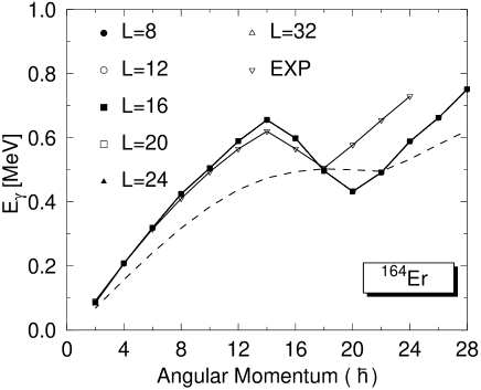
Figure 1: E_γ[MeV] versus angular momentum calculated for different values of $L$ in the Fomenko expansion, together with the experimental values and the HFB_e ones (dashed line). Notice that all points for different $L$ values lie on top of each other for all angular momenta.

We now turn to the problem of the divergences in calculations where the exchange terms are neglected. As we have seen in eq. (58) and in Appendix B, the poles appear whenever $u_{k}^{2}=v_{k}^{2}=1/2$ and $\varphi_{l}=\pi/2$. The first condition, obviously, can not be eluded. In the non-selfconsistent PAV method because the occupancies $v_{k}^{2}$ of the wave function are already determined by the solution of the HFB equations and in the self-consistent VAP because it would be against the variational principle. To investigate the behavior of the occupancies $v_{k}^{2}$, we have solved the selfconsistent cranked HFB_s equations along the Yrast band for the nucleus $\@@nuc{164}{Er}$. The wave functions $\Phi_{s}$ determined in this way have been analyzed in the canonical basis. In Fig. 2, we show the smallest values of the quantity $u_{k}^{2}-v_{k}^{2}$, for protons and neutrons, found in $\Phi_{s}$, as a function of the angular momentum. At small spins and up to spin 8 $\hbar$, the quantity $u_{k}^{2}-v_{k}^{2}$ for neutrons is rather small (around $-0.05$), at spin 10 $\hbar$ it reaches the critical value $u_{k}^{2}=v_{k}^{2}$ and from this point on it steadily increases up to the maximal value at a spin value of 28 $\hbar$. This behavior is typical of the high spin regime. At small angular momentum, the system is well paired and we may find a pair of nucleons close to the Fermi surface with $u_{k}^{2}\approx v_{k}^{2}$. As the spin increases the pairs align (states start being predominantly occupied or empty) and at high spins, when the pairing collapse takes place, the states become either fully occupied or empty. For protons the situation is even worse, we find two critical points, one around $I=12\hbar$ and the other around $I=22\hbar$.

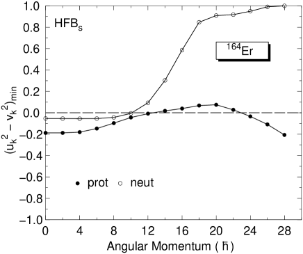
Figure 2: The smallest values of $(u_{k}^{2}-u_{k}^{2})$ along the Yrast line of $\@@nuc{164}{Er}$ for the HFB_s in the canonical basis.

The second condition for having the pole, i.e. that $\varphi_{l}=\pi/2$, is in principle avoidable, since $\varphi_{l}=\pi l/L$, taking L odd in the Fomenko expansion should be enough. This recipe, as we shall see below, helps in some cases but it does not guarantees that one is error free. The reason is very easy, to find convergence in the Fomenko expansion one must take L large enough, but then one may get too close to the critical $\pi/2$. That means in this way one avoids to get nonsense but the results may not be reliable. As we have seen above and in Appendix B, in the neighborhood of the poles we will get separately big contributions to the Hartree-Fock energy and to the pairing energy. If all exchange terms have been taken into account in the calculations, the sum of the divergent terms provides a finite value. This cancellation, however, is not guaranteed if some exchange terms have been neglected, as in the ${\rm HFB_{s}}$ approach, which we now discuss. In Table 1, we show for the nucleus $\@@nuc{164}{Er}$ the differences in the pairing, eq. (77), Hartree-Fock, eq. (75), and total, eq. (64), projected energies calculated for $L=8$ and $L=20$ (column labeled L-EVEN) and for $L=9$ and $L=21$ (column labeled L-ODD) as a function of the angular momentum. In the even-L calculations in the PAV_s approach, we find large $\Delta E$ values in the pairing and the HF energies around $I=10,12\hbar$ and $I=24\hbar$. These deviations do not cancel each other and give rise to large $\Delta E_{tot}$, indicating that no convergence is reached. For odd-L values the situation is much better. The largest $\Delta E_{tot}$ is around 20 keV which is more than one order of magnitude smaller than in the even-L case. Lastly, in the last column the difference of the total energy between $L=8$ and $L=9$ is displayed. We clearly observe that again large values around $I=10,12\hbar$ and $I=24\hbar$ are obtained. Interestingly, a comparison with fig. 2 shows that these spin values are those where $u_{k}^{2}-v_{k}^{2}$ is very small, i.e. the poles. The neutron system is responsible for the increase at $I=10\hbar$, see second column, and the proton one around $I=12\hbar$ and $I=24\hbar$.

	L-EVEN			L-ODD
I($\hbar$)	$\Delta E_{pai}$	$\Delta E_{hf}$	$\Delta E_{tot}$	$\Delta E_{pai}$	$\Delta E_{hf}$	$\Delta E_{tot}$	$E_{tot}^{8}-E_{tot}^{9}$
0	-1.12	-2.45	-3.55	1.46	0.94	2.39	5.8
2	-1.21	-2.43	-3.64	1.50	0.94	2.44	5.9
4	-1.71	-2.61	-4.31	1.86	1.02	2.88	7.0
6	-4.19	-3.62	-7.81	3.75	1.36	5.11	13.1
8	-11.76	-6.99	-18.76	8.55	1.80	10.35	31.6
10	57.62	-99.99	-42.37	12.67	0.31	12.98	71.0
12	-347.66	22.27	-325.39	8.40	-4.64	3.76	542.4
14	149.53	-10.35	139.17	-7.09	0.27	-6.81	-232.1
16	61.24	-6.07	55.17	-11.96	1.19	-10.77	-92.2
18	27.70	-3.33	24.37	-10.88	1.31	-9.57	-41.0
20	24.19	-3.12	21.07	-10.55	1.36	-9.19	-35.5
22	124.15	-15.49	108.66	-13.28	1.66	-11.62	-181.4
24	-144.09	17.41	-126.68	21.92	-2.65	19.27	211.8
26	-38.19	4.45	-33.75	21.73	-2.53	19.20	56.9
28	-9.22	1.01	-8.21	5.71	-0.63	5.09	13.4

Table 1: Differences (in keV) between the projected energies calculated with $L=9$ ($E_{i}^{9}$) and $L=21$ ($E_{i}^{21}$) and $L=8$ ($E_{i}^{8}$) and $L=20$ ($E_{i}^{20}$) in the Fomenko expansion for the nucleus $\@@nuc{164}{Er}$, calculated in the PAV_s approach. The last column displays the difference between the total energy calculated with $L=8$ and $L=9$.

¿From this table, we conclude that even-L values should be avoided and that the total energy for odd-L is a function of $L$. Usually, we are not interested in total energies but in relative ones, for instance in the $\gamma$-ray energy. Now the question is whether we can find a kind of plateau condition that provides us the optimal L-value for all $I$-values. In Fig. 3 we display the quantity $E_{\gamma}^{L}(I)/E_{\gamma}^{11}(I)$ as a function of $L$. We have chosen the value $L=11$ to normalize the $\gamma$-ray energies because it is large enough that in the absence of poles a good convergence would be found, and small enough that in the presence of poles we do not come too close to the critical $\varphi_{L}=\pi/2$. We found a good plateau for spin values 2 to $6\hbar$ and a rather good one for $I=16,18$ and $20\hbar$, the worst cases are for $I=14\hbar$ and $I=24\hbar$. This behavior is again strongly correlated with the nodes in Fig. 2. We observe that the largest deviations of the most reasonable values are about 7 %. It is clear that more sensitive quantities like second moments of inertia will show larger uncertainties.

All calculations of projected energies shown up to this point have been done with the prescription of eq. (33) for the density dependent part of the force, namely the projected density.

Figure 3: The transition energies E_γ[MeV] for a given angular momentum as a function of the parameter $L$ of the Fomenko expansion.

		DD1		DD2
I($\hbar$)	$\Delta E^{8-20}_{pai}$	$\Delta E^{8-20}_{hf}$	$\Delta E^{8-20}_{tot}$	$\Delta E^{8-20}_{hf}$	$\Delta E^{8-20}_{tot}$	$\Delta E^{9-21}_{tot}$
00	-17.27	17.28	0.01	-6.03	-23.30	-0.56
02	-26.45	26.45	0.01	-6.60	-33.05	-0.42
04	145.93	-145.92	0.01	-95.88	50.05	0.08
06	13.91	-13.90	0.01	18.93	32.85	1.21
08	6.24	-6.23	0.01	5.82	12.05	3.17
10	3.11	-3.11	0	2.61	5.72	3.16
12	1.15	-1.15	0	0.98	2.13	1.27
14	0.36	-0.36	0	0.32	0.68	0.38
16	0.12	-0.12	0	0.10	0.22	0.10
18	0.02	-0.02	0	0.02	0.04	0.01
20	0.01	-0.01	0	0.01	0.02	0
22	0	0	0	0	0.01	0
24	0	0	0	0	0	0
26	0	0	0	0	0	0
28	0	0	0	0	0	0

Table 2: Differences $\Delta E$ (in keV) between the projected energies calculated with $L=8$ ($E_{i}^{8}$) and $L=20$ ($E_{i}^{20}$) in the Fomenko expansion for the nucleus $\@@nuc{164}{Er}$ taking into account all the contributions of the force to the fields. [DD1] and [DD2] are meaning the prescription used for the density–dependent term. In the last column $\Delta E_{tot}$ is the difference between the projected energies calculated with $L=9$ and $L=21$.

We shall now discuss the convergence of our results with respect to the density dependence of the Hamiltonian used in the calculations. In order to isolate this issue, we do not neglect any exchange terms in the calculations, that means we solve the HFB_e equations. This provides us with the wave function $\Phi_{e}$ which we use to calculate the projected energy, which can calculated according to two prescriptions. Notice that $\Phi_{e}$ is different from $\Phi_{s}$ and that the levels occupancies of both wave functions are not necessarily the same. As it is shown in section B.1.1 the prescription using the projected density, which we shall label DD1, was divergence free, while the second prescription, the mixed density one (section B.1.2), from now on called DD2, was showing an integrable divergence. As in Table 1 we shall calculate separately the pairing and the Hartree-Fock contributions to the total energy. Since the density–dependent term does not contribute to the pairing energy (the parameter $x_{0}$ in the Gogny force is equal to $1$) this energy is independent of the prescription used for the density dependent term. In Table 2 we display the differences $\Delta E^{8-20}$ of projected energies calculated with the pairing energy, eq. (77), the HF energy, eq. (75) and the sum of both, the total energy. At low and medium spins, the difference of pairing energies for $L=8$ and 20 is not equal to zero indicating the known divergences. We find the largest value for $I=4\hbar$ indicating that the wave function $\Phi_{e}$ has a level occupancy at this spin value such that $u_{k}^{2}\approx v_{k}^{2}$. Inspection of the canonical basis indicates that the orbital is a neutron one, the proton system in this case does not have orbitals with $v_{k}^{2}$ close to 1/2. At high spins, the wave function $\Phi_{e}$ is not paired in the proton system (see ref. [18]) and in the neutron system it does not have orbitals with $v_{k}^{2}$ close to 1/2. To get convergence, either with the DD1 or the DD2 prescription, the difference of the total energy calculated with different L values, must be zero. This is the case in the DD1 approach where, even with even-L values, the HF energy differences are almost exactly the same as the pairing ones. As a result, both cancel out and the total energy is convergent, as expected. With the DD2 prescription and even-L values, however, the HF results are different from the pairing ones and as a result no convergence for the total energy is found. We know, however, that the DD2 divergence is integrable, that means if the integral is carefully performed the convergence must be found. This is what happens if we do the calculations with odd-L values (see last column) where the largest deviation found is 3 keV. Obviously, more sophisticated integration methods will provide better convergence.

An interesting point concerning the density prescriptions DD1 and DD2 is to know if there is a big difference in the results calculated with DD1 or DD2. In Fig. 4 we show the $\gamma$-ray energies along the yrast line of the nucleus ¹⁶⁴Er in the HFB_e with the DD1 (in the figure PAV1) and with DD2 (in the figure PAV2). As we can see the behavior is very similar and the physics is clearly the same. A similar conclusion was found in [15] in the Lipkin-Nogami approach.

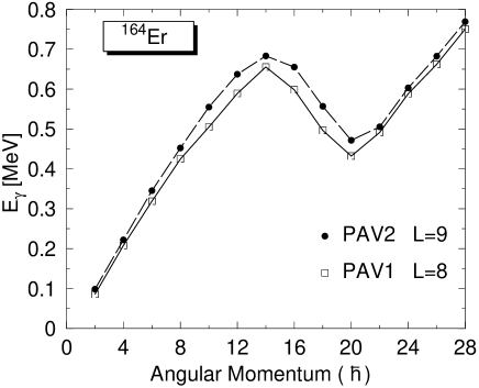
Figure 4: E_γ[MeV] versus angular momentum for both prescriptions of the density.

6 The variation after projection method : The nuclei ⁴⁸Cr and ⁵⁰Cr

In ref. [24] and [25] a good agreement between the HFB approximation, the exact shell model diagonalization and the experimental results was found for the rotational states of the nuclei ⁴⁸Cr and ⁵⁰Cr. Only the $\gamma$-ray energies along the yrast bands in the HFB approach were systematically around 0.5 MeV smaller than experimentally observed. A simulation with the exact shell model diagonalization in [24] showed that the shift was due to a deficient treatment of the pairing correlations of the HFB method in the weak pairing regime. It is well known that the variation after projection method is able to provide pairing correlations even at the limiting case when the HFB approach collapses to the HF one. In this section we shall investigate the mentioned nuclei in the VAP method.

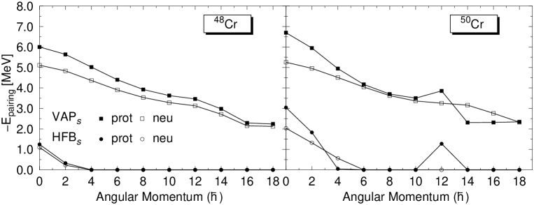
Figure 5: Pairing correlation energies in the HFB_s and VAP_s approaches for the nucleus ⁴⁸Cr and ⁵⁰Cr respectively.

The HFB calculations of refs. [24] and [25] were performed in the standard approximation, i.e. HFB_s. For nuclei like these with little pairing -low level density at the Fermi surface- is very unlikely to find orbitals with $v_{k}^{2}=u_{k}^{2}$, nevertheless we have checked during the minimization process of the VAP_s that no orbitals were populated in that way. Additionally, we have performed also the HFB_e and the VAP_e calculations. In Fig. 5, we represent the HFB_s and VAP_s (see eq.(77)) pairing energies for the nuclei ⁴⁸Cr, left hand side, and ⁵⁰Cr, right hand side. In the HFB_s approach the pairing energies are rather small, for ⁴⁸Cr practically zero for all spin values, with the exception of the $I=0$ and $2\hbar$ values where they are very small. For ⁵⁰Cr they are also very small and only for $I=0,2,4$ and $12\hbar$ differ from zero. In both nuclei we find the Coriolis antipairing effect that leads to a sharp transition from a (weakly) superfluid system to a normal one. The VAP_s solutions, on the other hand, are well paired and no sharp transition is seen, only a smooth decrease in the correlation energy is found.

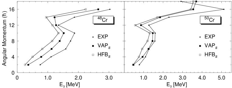
Figure 6: The transition ${\gamma}$-ray energies versus the angular momentum in the HFB_s and VAP_s approaches for the nucleus ⁴⁸Cr and ⁵⁰Cr. The experimental results are also shown.

In Fig. 6, the ${\gamma}$-ray energies along the yrast band are displayed in the HFB_s and VAP_s approaches together with the experimental results for ⁴⁸Cr, [26] and ⁵⁰Cr, [27]. As discussed in [24], the HFB_s ${\gamma}$-ray energies for ⁴⁸Cr show the same trend as the experimental ones but are about 0.5 MeV smaller. The VAP_s approach, on the other hand, due to the larger pairing energy leads to smaller moment of inertia improving the agreement with the experiment. The VAP_s results come closer to the experiment and the backbending is slightly better described. For ⁵⁰Cr the situation is similar, the VAP_s approach improves considerably the HFB_s one specially at low and medium spins. One may ask, however, why we do not get enough pairing correlations in the VAP_s method as to match the experimental results. There are several possible answers, first in our calculations we do not include p-n pairing which is known [28] to play an important role in these nuclei. Second, the fact that in these nuclei, in the HFB approximation, there are barely any pairing correlations indicates that the potential energy curve is rather flat against pairing fluctuations. This kind of fluctuations is not included in the PNP method.

In Figs. 7 and 8, we finally present the results of the exact HFB calculations, HFB_e, and the corresponding VAP_e method. The pairing correlation energies are represented in Fig. 7. As expected [18], the neglected pairing terms in the HFB_s approach have an antipairing effect, mainly the Coulomb term. The small pairing energy of the HFB_s approach is quenched in the HFB_e, in particular the proton pairing energies completely vanish. The pairing energies in the VAP_e approach display this effect even more clearly. The total VAP_e pairing energy is considerably reduced with respect to the VAP_s approach. Furthermore, while in the VAP_s the proton pairing energy is always larger than the neutron one in the VAP_e the proton pairing energy becomes always smaller than the neutron one.

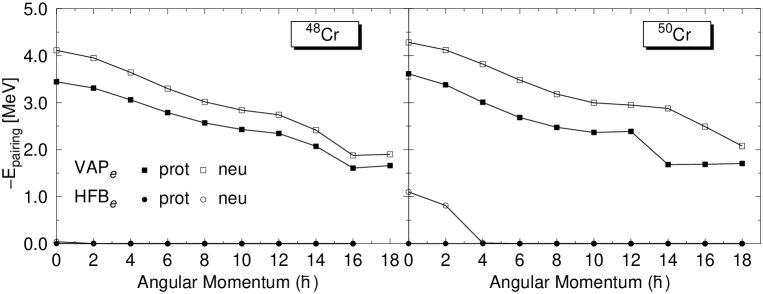
Figure 7: Pairing correlation energies in the HFB_e and VAP_e approaches for the nuclei ⁴⁸Cr and ⁵⁰Cr respectively.

In Fig. 8 we finally present the $\gamma$-ray energies in the HFB_e and the VAP_e together with the experimental ones. Since the pairing energies are negligible in the HFB_e and HFB_s for both nuclei, both sets of $\gamma$-ray energies practically coincide. With respect to the VAP_e values they are of the same quality as the VAP_s though somewhat smaller than these one, as expected from the behavior of the pairing correlations.

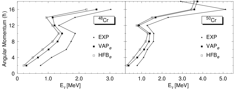
Figure 8: The transition ${\gamma}$-ray energies versus the angular momentum in the HFB_e and VAP_e approaches for the nuclei ⁴⁸Cr and ⁵⁰Cr. The experimental results are also shown.

7 Conclusions.

In this paper we have derived the expressions needed to perform a particle number projected HFB calculation with a finite–range and density dependent force in the triaxial basis. We have studied and thoroughly discussed the divergences that appear for special values of orbital occupancies when exchange terms are neglected. We have performed exact and approximate calculations (neglecting some exchange terms) and found that in the latter case some problems associated with the convergence of the particle number projection arise leading in some cases to an inaccuracy of about 10 % in the values of the $\gamma$-ray energies. Interestingly, all terms of the force, even of the Coulomb part, must be taken into account. This feature presents a challenge for interactions where a given force is used in the particle-hole channel and a different one in the particle-particle channel.

We have furthermore performed variation after the projection for the ^48,50Cr nuclei with the Gogny force. We found strong pairing correlations, at variance with the weekly correlated HFB approach. These correlations smoothly decrease with increasing angular momentum indicating that no sharp phase transition takes place as predicted by the HFB approach. The projected calculations improve the HFB ones but some correlations (probably T=0 pairing) not present in our approach are still missing.

Appendix A Appendix A: The Gogny Force.

In the calculations we use the Gogny interaction [29] as the effective force . The main ingredients of this force are the phenomenological density dependent term which was introduced to simulate the effect of a G–matrix interaction and the finite range of the force which allows to obtain the Pairing and Hartree–Fock fields from the same interaction. We use the parametrization D1S, which was fixed by Berger et al. [30]. The force is given by

$$v_{12} = \sum_{i=1}^{2}e^{-{(\vec{r}_{1}-\vec{r}_{2})}^{2}/\mu_{i}^{2}}(W_{i}+B_{i}P_{\sigma}-H_{i}P_{\tau}-M_{i}P_{\sigma}P_{\tau})+$$ (60)

$$+ W_{LS}(\vec{\sigma}_{1}+\vec{\sigma}_{2})\vec{k}\times\delta(\vec{r}_{1}-\vec{r}_{2})\vec{k}+$$

$$+ t_{3}(1+x_{0}P_{\sigma})\delta(\vec{r}_{1}-\vec{r}_{2})\rho^{1/3}\left(\frac{1}{2}(\vec{r}_{1}+\vec{r}_{2})\right),$$

and the Coulomb force

$$v_{12}^{C}=(1+2\tau_{1z})(1+2\tau_{2z})\frac{e^{2}}{|\vec{r}_{1}-\vec{r}_{2}|}.$$ (61)

The density operator, $\hat{\rho}(\vec{r})$, is given by

$$\hat{\rho}(\vec{r})=\sum_{i=1}^{A}\delta(\vec{r}-\vec{r}_{i})=\sum_{ij}\phi_{i}^{*}(\vec{r})\phi_{j}(\vec{r})\langle S_{i}|S_{j}\rangle c_{i}^{\dagger}c_{j}=\sum_{ij}f_{ij}(\vec{r})c_{i}^{\dagger}c_{j}\,.$$ (62)

In the two-body interaction used in the calculations we also include the one–body and two–body center of mass corrections.

$$\hat{T}=\sum_{i}\frac{{\vec{p}_{i}}^{\,2}}{2m}\left(1-\frac{1}{A}\right)-\frac{1}{Am}\sum_{i>j}\,\vec{p}_{i}\cdot\vec{p}_{j}$$ (63)

Appendix B Appendix B: Calculation of the projected energy in the canonical basis.

In this appendix we show that the projected energy is always well–defined if the direct (Hartree), exchange (Fock) and pairing terms of each component of the force are taken into account, i.e. if no exchange terms are neglected.

The projected energy can be written in the following way 

$$E^{P}=Tr(t\rho^{P})+E^{P}_{hf}+E^{P}_{g}$$ (64)

where

$$E^{P}_{hf} = \frac{1}{2}\sum_{k_{1}k_{2}k_{3}k_{4}}\bar{v}_{k_{1}k_{2}k_{3}k_{4}}\sum_{l}y_{l}\,\rho_{k_{3}k_{1}}(\varphi_{l})\rho_{k_{4}k_{2}}(\varphi_{l})$$ (65)

$$E^{P}_{g} = \frac{1}{4}\sum_{k_{1}k_{2}k_{3}k_{4}}\bar{v}_{k_{1}k_{2}k_{3}k_{4}}\sum_{l}y_{l}\,\kappa^{01}_{k_{1}k_{2}}(\varphi_{l})\kappa^{10}_{k_{3}k_{4}}(\varphi_{l})$$ (66)

These energies are given in terms of the $\varphi_{l}$-dependent density matrix $\rho(\varphi_{l})$ and the pairing tensors $\kappa^{01}(\varphi_{l})$ and $\kappa^{10}(\varphi_{l})$. These quantities can be easily evaluated in the canonical basis. In this basis, denoted by $\{a,a^{\dagger}\}$, the usual density matrix $\rho_{{k_{1}}{k_{2}}}=\langle\Phi|a_{k_{2}}^{\dagger}a_{k_{1}}|\Phi\rangle$ is diagonal and the usual pairing tensor $\kappa_{{k_{1}}{k_{2}}}=\langle\Phi|a_{k_{2}}a_{k_{1}}|\Phi\rangle$ has the canonical form. In this basis the quantities we are interested in are given by

$$\rho_{k_{1}k_{2}}(\varphi_{l}) = \frac{\langle\Phi|a_{k_{2}}^{\dagger}a_{k_{1}}e^{{\mathrm{i}}\varphi_{l}\hat{N}}|\Phi\rangle}{\langle\Phi|e^{{\mathrm{i}}\varphi_{l}\hat{N}}|\Phi\rangle}$$

$$\kappa^{01}_{k_{1}k_{2}}(\varphi_{l}) = \frac{\langle\Phi|a_{k_{1}}^{\dagger}a_{k_{2}}^{\dagger}e^{{\mathrm{i}}\varphi_{l}\hat{N}}|\Phi\rangle}{\langle\Phi|e^{{\mathrm{i}}\varphi_{l}\hat{N}}|\Phi\rangle},\quad\quad\kappa^{10}_{k_{1}k_{2}}(\varphi_{l})=\frac{\langle\Phi|a_{k_{2}}a_{k_{1}}e^{{\mathrm{i}}\varphi_{l}\hat{N}}|\Phi\rangle}{\langle\Phi|e^{{\mathrm{i}}\varphi_{l}\hat{N}}|\Phi\rangle}.$$ (67)

These matrix elements can be easily evaluated

$$\langle\Phi|e^{{\mathrm{i}}\varphi_{l}\hat{N}}|\Phi\rangle = \prod_{k>0}\langle-|(u_{k}+v_{k}a_{\bar{k}}a_{k})e^{{\mathrm{i}}\varphi_{l}\hat{N}}(u_{k}+v_{k}a_{k}^{\dagger}a_{\bar{k}}^{\dagger})|-\rangle$$

$$= \prod_{k>0}\langle-|(u_{k}+v_{k}a_{\bar{k}}a_{k})(u_{k}+v_{k}e^{2{\mathrm{i}}\varphi_{l}}a_{k}^{\dagger}a_{\bar{k}}^{\dagger})|-\rangle$$

$$= \prod_{k>0}(u_{k}^{2}+v_{k}^{2}e^{2{\mathrm{i}}\varphi_{l}})|-\rangle,$$

here $\bar{k}$ denotes the canonical conjugated state of $k$. To calculate $\langle\Phi|a_{k_{2}}^{\dagger}a_{k_{1}}e^{{\mathrm{i}}\varphi_{l}\hat{N}}|\Phi\rangle$, we shall proceed in the same way. Let us first assume $k_{2}\neq k_{1}$, then

$$\langle\Phi|a_{k_{2}}^{\dagger}a_{k_{1}}e^{{\mathrm{i}}\varphi_{l}\hat{N}}|\Phi\rangle=\prod_{k>0}\langle-|(u_{k}+v_{k}a_{\bar{k}}a_{k})a_{k_{2}}^{\dagger}a_{k_{1}}(u_{k}+v_{k}e^{2{\mathrm{i}}\varphi_{l}}a_{k}^{\dagger}a_{\bar{k}}^{\dagger})|-\rangle=0,$$ (69)

that means, the $\varphi_{l}$-dependent density matrix $\rho_{{k_{1}}{k_{2}}}(\varphi_{l})$, like the normal density matrix $\rho_{{k_{1}}{k_{2}}}$, is diagonal in the canonical basis. For $k_{2}=k_{1}=k$ we obtain

$$\langle\Phi|a_{k}^{\dagger}a_{k}e^{{\mathrm{i}}\varphi_{l}\hat{N}}|\Phi\rangle=v_{k}^{2}\cdot e^{2{\mathrm{i}}\varphi_{l}}\cdot\prod_{m>0,m\neq k}(u_{m}^{2}+v_{m}^{2}e^{2{\mathrm{i}}\varphi_{l}}).$$ (70)

Therefore, in the canonical basis, the matrix $\rho_{km}(\varphi_{l})$ is given by

$$\rho_{km}(\varphi_{l})=\delta_{km}\cdot\frac{v_{k}^{2}\cdot e^{2{\mathrm{i}}\varphi_{l}}}{u_{k}^{2}+v_{k}^{2}e^{2{\mathrm{i}}\varphi_{l}}}.$$ (71)

We see in this expression that for $u_{k}=v_{k}$ and $\varphi_{l}=\pi/2$, the matrix element diverges and one has to be very careful in the calculations. It is easy to show that $\rho_{\bar{k}\bar{m}}(\varphi_{l})=\rho_{km}(\varphi_{l})$ .

Let us now calculate the $\varphi_{l}$-dependent pairing tensors in the canonical basis

$$\langle\Phi|a_{k_{2}}^{\dagger}a_{k_{1}}^{\dagger}e^{{\mathrm{i}}\hat{N}\varphi_{l}}|\Phi\rangle = \prod_{m>0}\langle-|(u_{m}+v_{m}a_{\bar{m}}a_{m})a_{k_{2}}^{\dagger}a_{k_{1}}^{\dagger}(u_{m}+v_{m}a_{m}^{\dagger}a_{\bar{m}}^{\dagger}e^{2{\mathrm{i}}\varphi_{l}}|-\rangle$$ (72)

$$= \delta_{k_{1}\bar{k}_{2}}u_{k_{2}}v_{k_{2}}\prod_{m>0,m\neq k_{2}}(u_{m}^{2}+v_{m}^{2}\cdot e^{2{\mathrm{i}}\varphi_{l}})$$

in the same way

$$\langle\Phi|a_{k_{1}}a_{k_{2}}e^{{\mathrm{i}}\varphi_{l}\hat{N}}|\Phi\rangle=\delta_{k_{1}\bar{k}_{2}}u_{k_{2}}v_{k_{2}}\prod_{m>0,m\neq k_{2}}(u_{m}^{2}+v_{m}^{2}\cdot e^{2{\mathrm{i}}\varphi_{l}}).$$ (73)

The non-zero matrix elements are given by

$$\kappa_{k\bar{k}}^{01}=\frac{u_{k}v_{k}}{u_{k}^{2}+v_{k}^{2}\,e^{2{\mathrm{i}}\varphi_{l}}},\quad\quad\quad\kappa_{k\bar{k}}^{10}=\frac{u_{k}v_{k}e^{2{\mathrm{i}}\varphi_{l}}}{u_{k}^{2}+v_{k}^{2}\,e^{2{\mathrm{i}}\varphi_{l}}}$$ (74)

obviously, $\kappa_{k\bar{k}}^{01}=-\kappa_{\bar{k}k}^{01}$ and $\kappa_{k\bar{k}}^{10}=-\kappa_{\bar{k}k}^{10}$. Again the dangerous terms are for $u_{k}=v_{k}$ and $\varphi_{L}=\pi/2$.

¿From eq. (65) and using the expressions derived above, we obtain

$$E_{hf}^{P} = \frac{1}{2}\sum_{k_{1}k_{2}k_{3}k_{4}}{\bar{v}}_{k_{1}k_{2}k_{3}k_{4}}\sum_{l}y_{l}\rho_{kk}(\varphi_{l})\delta_{k_{3}k}\delta_{k_{1}k}\rho_{k^{\prime}k^{\prime}}(\varphi_{l})\delta_{k_{4}k^{\prime}}\delta_{k_{2}k^{\prime}}$$ (75)

$$= \frac{1}{2}\sum_{k,k^{\prime}}{\bar{v}}_{kk^{\prime}kk^{\prime}}\cdot\sum_{l}y_{l}\rho_{kk}(\varphi_{l})\rho_{k^{\prime}k^{\prime}}(\varphi_{l})$$

$$= \frac{1}{2}\sum_{k,k^{\prime}>0}({\bar{v}}_{kk^{\prime}kk^{\prime}}+{\bar{v}}_{\bar{k}k^{\prime}\bar{k}k^{\prime}}+{\bar{v}}_{k\bar{k^{\prime}}k\bar{k^{\prime}}}+{\bar{v}}_{\bar{k}\bar{k^{\prime}}\bar{k}\bar{k^{\prime}}})\sum_{l}y_{l}\rho_{kk}(\varphi_{l})\rho_{k^{\prime}k^{\prime}}(\varphi_{l}).$$

Taking into account that $y_{l}(\varphi_{l})\approx\langle\Phi|e^{{\mathrm{i}}\varphi_{l}\hat{N}}|\Phi\rangle$, we see that the possible poles of $\rho_{kk}(\varphi_{l})$ and $\rho_{k^{\prime}k^{\prime}}(\varphi_{l})$ are canceled when $k\neq k^{\prime}$, i.e. we may only have problems if $k=k^{\prime}$. The contribution to the Hartree- Fock energy in this case is given by

$$[E_{hf}^{P}]_{pole} = \sum_{k>0}\sum_{l}{\bar{v}}_{k\bar{k}k\bar{k}}\,\,y_{l}\frac{v_{k}^{4}e^{4{\mathrm{i}}\varphi_{l}}}{{(u_{k}^{2}+v_{k}^{2}e^{2{\mathrm{i}}\varphi_{l}})}^{2}}$$ (76)

$$= {\mathcal{N}}\sum_{k>0}\sum_{l}{\bar{v}}_{k\bar{k}k\bar{k}}\frac{v_{k}^{4}e^{4{\mathrm{i}}\varphi_{l}}}{{(u_{k}^{2}+v_{k}^{2}e^{2{\mathrm{i}}\varphi_{l}})}}\cdot\prod_{m>0,m\neq k}(u_{m}^{2}+v_{m}^{2}e^{2{\mathrm{i}}\varphi_{l}}).$$

where we have made use of eq. (5) and ${\mathcal{N}}=\left[\sum_{l=1}^{L}\langle{\Phi}|e^{i\varphi_{l}\hat{N}}|\Phi\rangle\right]^{-1}$. This contribution clearly diverges for $u_{k}^{2}=v_{k}^{2}$ and $\varphi_{l}=\pi/2$. The pairing energy term is given by eq. (66), in the canonical basis it takes the form

$$E_{pai}^{P} = \frac{1}{4}\sum_{k,k^{\prime}>0}\sum_{l}y_{l}({\bar{v}}_{\bar{k}k\bar{k}^{\prime}k^{\prime}}\kappa_{\bar{k}k}^{01}\kappa_{\bar{k}^{\prime}k^{\prime}}^{10}+{\bar{v}}_{k\bar{k}\bar{k}^{\prime}k^{\prime}}\kappa_{k\bar{k}}^{01}\kappa_{\bar{k}^{\prime}k^{\prime}}^{10}+$$ (77)

$$+ {\bar{v}}_{\bar{k}kk^{\prime}\bar{k}^{\prime}}\kappa_{\bar{k}k}^{01}\kappa_{k^{\prime}\bar{k}^{\prime}}^{10}+{\bar{v}}_{k\bar{k}k^{\prime}\bar{k}^{\prime}}\kappa_{k\bar{k}}^{01}\kappa_{k^{\prime}\bar{k}^{\prime}}^{10})$$

$$= \sum_{kk^{\prime}>0}\sum_{l}y_{l}{\bar{v}}_{k\bar{k}k^{\prime}\bar{k}^{\prime}}\kappa_{k\bar{k}}^{01}\kappa_{k^{\prime}\bar{k}^{\prime}}^{10}.$$

As before, $y_{l}$ cancels one possible pole, and if $k=k^{\prime}$ the contribution to the energy is

$$[E_{g}^{P}]_{pole} = \sum_{k>0}\sum_{l}{\bar{v}}_{k\bar{k}k\bar{k}}\,\,y_{l}\frac{u_{k}^{2}v_{k}^{2}e^{2{\mathrm{i}}\varphi_{l}}}{{(u_{k}^{2}+v_{k}^{2}e^{2{\mathrm{i}}\varphi_{l}})}^{2}}$$ (78)

$$= {\mathcal{N}}\sum_{k>0}\sum_{l}{\bar{v}}_{k\bar{k}k\bar{k}}\frac{u_{k}^{2}v_{k}^{2}e^{2{\mathrm{i}}\varphi_{l}}}{{(u_{k}^{2}+v_{k}^{2}e^{2{\mathrm{i}}\varphi_{l}})}}\cdot\prod_{m>0,m\neq k}(u_{m}^{2}+v_{m}^{2}e^{2{\mathrm{i}}\varphi_{l}})$$

which also diverges for $u_{k}^{2}=v_{k}^{2}$ and $\varphi_{l}=\pi/2$. The total contribution to the energy is given by the sum of eq.(76) and eq.(78), we obtain

$$[E_{hf}^{P}]_{pole}+[E_{g}^{P}]_{pole} = \sum_{k>0}\sum_{l}{\bar{v}}_{k\bar{k}k\bar{k}}\,\,\frac{y_{l}v_{k}^{2}e^{2{\mathrm{i}}\varphi}}{{(u_{k}^{2}+v_{k}^{2}e^{2{\mathrm{i}}\varphi_{l}})}^{2}}$$ (79)

$$= {\mathcal{N}}\sum_{k>0}\sum_{l}{\bar{v}}_{k\bar{k}k\bar{k}}v_{k}^{2}e^{2{\mathrm{i}}\varphi_{l}}\cdot\prod_{m>0,m\neq k}(u_{m}^{2}+v_{m}^{2}e^{2{\mathrm{i}}\varphi_{l}})$$

which clearly does not diverge at $u_{k}^{2}=v_{k}^{2}$ and $\varphi_{l}=\pi/2$.

This result shows that in case of particle number projection one cannot arbitrarily neglect exchange terms of any component of the two-body potential, including the Coulomb one.

B.1 Density–dependent interactions.

In the previous demonstration we have not considered the case of density–dependent interactions $\bar{v}_{k_{1}k_{2}k_{3}k_{4}}$ in the analysis of the convergence. We shall distinguish between the two choices for the Hamiltonian density in order to study this problem.

B.1.1 Projected density.

Taking into account the expression (33), one sees that the density–dependent energy depends only on the proton and neutron projected densities. We must therefore analyze the behavior of these densities in the presence of poles. The projected density is given by

$$\rho^{P}_{k_{1}k_{2}} = \sum_{l}y_{l}\rho_{k_{1}k_{2}}(\varphi_{l}).$$ (80)

As we saw in the previous section, any pole of $\rho_{k_{1}k_{2}}(\varphi_{l})$ will be canceled by a zero of the same order from the factor $y_{l}$. Therefore, if we take the projected density for the density dependent term, the total energy including this term is well–defined.

B.1.2 Mixed density.

In this case the energy of the density–dependent term is given by eq. (37). As we can see in this expression and in eq. (39), the densities $\rho(\varphi_{l_{\tau})}$ and the norms $y_{l_{\tau}}$ appear pairwise indicating a cancellation of possible poles and zeros. However, problems may arise if the interaction ${V}_{DD}$ itself has some poles. In this prescription ${V}_{DD}$ depends on $\rho(\vec{r},\varphi_{l})$ given by eq. (36). Writing the density matrix elements in the canonical basis we find that

$$\rho(\vec{r},\varphi_{l})=\sum_{k}\left(f_{kk}\left(\vec{r}\right)+f_{\bar{k}\bar{k}}\left(\vec{r}\right)\right)\frac{v_{k}^{2}e^{2i\varphi_{l}}}{u_{k}^{2}+v_{k}^{2}e^{2i\varphi_{l}}}$$ (81)

where the functions $f_{kk^{\prime}}(\vec{r})$ are defined in eq. (62). Clearly, if one of the $v_{k}^{2}$, let’s say $v_{k_{0}}^{2}$, equals $1/2$ then the density is singular at $\varphi_{l}=\pi/2$ and in the neighborhood of this point it behaves as

$$\rho(\vec{r},\varphi_{l})\sim-\frac{i}{2}\left(f_{k_{0}k_{0}}\left(\vec{r}\right)+f_{\overline{k}_{0}\overline{k}_{0}}\left(\vec{r}\right)\right)\frac{1}{\left(\varphi_{l}-\pi/2\right)}$$ (82)

which is clearly divergent. This singularity, however, does not pose any real drawback as the density dependence of the interaction is proportional to $\rho(\vec{r},\varphi_{l})^{\alpha}$ with $\alpha=1/3$ and therefore the singularity is integrable.

References

[1] P. Ring and P. Shuck, The Nuclear Many Body Problem
(Springer-Verlag, Berlin, 1980).
[2] K. Dietrich, H. J. Mang and J. H. Pradal,
Phys. Rev. 135 (1964) B22.
[3] J.L. Egido, H.J. Mang, P. Ring,
Nucl. Phys. A 339 (1980) 390-414.
[4]
J. L. Egido and P. Ring,
Nucl. Phys. A 383, 189 (1982);
Nucl. Phys. A 388, 19 (1982).
[5] H.J. Lipkin,, Ann. Phys. (NY) 12 (1960) 425;
Y. Nogami Phys. Rev. B 134 (1964)313
[6]
B. Gall, P. Bonche, J. Dobaczeski, H. Flocard, P. H. Heenen,
Z. Phys. A 348(1994) 183 .
[7]
P. Bonche, H. Flocard, P. H. Heenen,
Nucl. Phys. A 598, 169 (1996).
[8] A. Valor, J.L. Egido and L. M. Robledo,
Phys. Rev. C 53 (1996) 172.
[9]A.V. Afanasjev et al., Nucl. Phys. A 676(2000) 196.
[10]
J. Dechargé and D. Gogny,
Phy. Rev. C 21(1980) 1568 .
[11]V.N. Fomenko. J. Phys. (G.B) A 3 (1970) 8.
[12]
R. Balian and E. Brezin, Nuovo Cimento 64 (1969) 37.
[13] A. Valor. J. L. Egido and L. M. Robledo,
Nucl. Phys. A 665(2000)46-70.
[14]
P. Bonche, J. Dobaczeski, H. Flocard, P. H. Heenen and J. Meyer, Nucl.
Phys. A 510 (1990) 466.
[15] A. Valor, J.L. Egido and L. M. Robledo,
Phys. Lett. B 392 (1997) 249.
[16]
J.L. Egido, J. Lessing, V. Martin and L.M. Robledo, Nucl. Phys.
A 594 (1995) 70.
[17] F. Doenau,
Phy. Rev. C 58 (1998) 872.
[18] M. Anguiano, J.L. Egido and L.M. Robledo,
Nucl. Phys. A 683 (2001)227-254.
[19] M. Girod and B. Grammaticos,
Phys. Rev. C 27 (1983) 2317.
[20]
J. L. Egido and L. M. Robledo,
Phys. Rev. Lett. 70 (1993) 2876.
[21]
A.L. Goodman, in Advances in Nuclear Physics 11 (1979) 263.
[22] K. W. Schmid and F. Gruemmer,
Rep. Prog. Phys. 50 (1987) 731.
[23] E.N. Shurshikov and N.V. Timofeeva,
Nuclear Data Sheets 65 (1992)365.
[24] E. Caurier, J.L. Egido, G. Martinez-Pinedo, A. Poves, J.
Retamosa, L. M. Robledo and A. Zuker, Phys. Rev. Lett.75, 2466
(1995)
[25] G. Martinez-Pinedo, A. Poves, L. M. Robledo,
E. Caurier, F. Nowacki, J. Retamosa and A. Zuker, Phys. Rev. C54, R2150 (1996)
[26] J.A. Cameron et al., Phys. Rev C49, 1347 (1994); J.A. Cameron et
al., Phys. Lett. B319, 58 (1993); T.W. Burrows, Nucl. Data Sheets 68, 1
(1993).
[27] T.W. Burrows, Nuclear Data Sheets (1990); S.M. Lenzi et al.,
Phys. Rev C56, 1313 (1997).
[28] A. Poves and G. Martinez-Pinedo,
Phys. Lett. B430 (1998)203.
[29] D. Gogny, in “Nuclear selfconsistent fields”, Eds.
G. Ripka and M. Porneuf (North Holland, 1975).
[30]
J. F. Berger, M. Girod and D. Gogny,
Comp. Phys. Comm. 63, 365 (1991).