Ground state particle-particle correlations and double beta decay

Abstract

A self-consistent formalism for the double beta decay of Fermi type is provided. The particle-particle channel of the two-body interaction is considered first in the mean field equations and then in the QRPA. The resulting approach is called the QRPA with a self-consistent mean field (QRPASMF). The mode provided by QRPASMF, does not collapse for any strength of the particle-particle interaction. The transition amplitude for double beta decay is almost insensitive to the variation of the particle-particle interaction. Comparing it with the result of the standard $pnQRPA$, it is smaller by a factor 6. The prediction for transition amplitude agrees quite well with the exact result. The present approach is the only one which produces a strong decrease of the amplitude and at the same time does not alter the stability of the ground state.

I Introduction

Many body theories have been very successful in describing the collective properties of nuclear systems [1, 2, 3, 4, 5, 6, 7, 8, 9, 10, 11, 12]. Many properties are described by considering only the two-body interaction between protons or between neutrons. However there are several features which cannot be explained if one ignores the interactions of protons and neutrons [13, 14, 15, 16, 17, 18, 19, 20, 21, 22, 23, 24, 25, 26]. For example the pairing interaction between protons and neutrons seems to be important for determining both the ground state and the high spin states properties of nuclei having $Z=N$ [18, 20, 22, 25]. The monopole and dipole proton-neutron interaction was intensively studied in connection with the double beta decay process [27, 28, 29, 30]. This subject was considered by many theoreticians especially in connection to the neutrino-less double beta decay ($0\nu\beta\beta$). Indeed, this phenomenon if it exists, might be crucial for answering a fundamental question of physics, namely whether the neutrino is a Majorana or a Dirac particle. In order to make predictions in this field one needs reliable tests for the nuclear matrix elements. Unfortunately, up to date, such tests are missing. However, since essentially the same matrix elements are used for the two neutrino double beta decay ($2\nu\beta\beta$) for which plenty of data exist, the idea of using those NN interactions, which provide a realistic description of the $2\nu\beta\beta$ process has been widely adopted. The present status of the theories proposed for $2\nu\beta\beta$ is as follows: The approach which produces results closest to experimental data is the proton-neutron quasiparticle random phase approximation ($pnQRPA$). The predictions for the transition amplitude is however too high comparing it to the existent data. Therefore one has looked for modifications of the existent formalism in order to obtain the desired quenching of the theoretical result. The first new approach was proposed by Cha [31] for a related subject. Indeed he noticed that the single beta transition rate is very sensitive to varying the strength of the two-body interaction in the particle-particle (pp) channel. This idea was adopted by most of the groups working in the field of $2\nu\beta\beta$ [32, 33, 34, 35, 36]. The results are as follows: The transition amplitude is almost insensitive to the variation of the strength, $g_{pp}$, with which one multiplies the matrix elements of a realistic force, of the pp interaction for a large interval starting from zero. Then the amplitude is decreasing quickly reaching zero for $g_{pp}\approx 1$ which, as a matter of fact is very closed to its critical value where the $pnQRPA$ breaks down. It should be mentioned that $g_{pp}=1$ is just what a realistic force produces. Of course on the fast down sloping part of the plot the experimental data is met so one could assume that the problem is solved. However, in this region the $pnQRPA$ is not a good approach since the results are not stable against adding new correlations. A positive feature of the $pnQRPA$ is that the Ikeda sum rule (ISR) is fully satisfied for any value of $g_{pp}$. Several attempts have been made to stabilize the $pnQRPA$ ground state, or to move the value zero of the transition amplitude to the unrealistic region. Among the proposed approaches are the boson expansion technique (BE) [37, 38], the multiple commutators method (MCM)[39, 40], the renormalized $pnQRPA$ [41] and the fully renormalized $pnQRPA$ [42]. The first three methods succeed to shift the zero of the transition amplitude to the unphysical region but the Ikeda sum rule is violated by an amount ranging from 15 to 30%. Some complementary features of the boson expansion and re-normalization procedure were studied in ref.[43]. Ikeda sum rule is the difference of the total strengths for beta minus and beta plus transitions and is influenced by the completeness of the states participating in the process as well as by the correlations involved in the ground state. Some groups consider Ikeda sum rule as a signature for the fact that the formalism takes care of the Pauli principle [44]. However, even if the Pauli principle is preserved, ISR can be violated if the states involved do not have a good particle number.

Very recently we started investigating the consistency of the $pnQRPA$ treatment of the pp interaction and the structure of the mean field [45, 46]. Indeed, without exception all previous formalisms included the particle-particle proton-neutron interaction in the $pnQRPA$ approach but ignored this interaction when the mean field was defined. In the previous paper we investigated this problem within a consistent approach. We have proved that including the particle-particle interaction in the single particle mean field prevents the QRPA to collapse when the interaction strength is increased, despite the attractive character of the pp interaction. Moreover the RPA energy is an increasing function of the interaction strength. Here we shall call the procedure mentioned above as the QRPA with a self-consistent mean field, QRPASMF.

In the present paper we study the double beta Fermi decay by using the wave functions provided by the QRPASMF approach. We are studying the Fermi transition since this has the nice feature that for a single j case, the model is exactly solvable and therefore one can test the accuracy of the adopted approximations. The paper is organized as follows: In Section 2 we review briefly the results obtained in the previous paper. On this occasion we collect the main results needed for the present purposes. In Section 3, the QRPA formalism is written for the quasiparticle operators which admit the generalized BCS wave function as vacuum. As we showed in ref.[46] the generalized BCS wave function is the static ground state of the system under consideration. The exact treatment is presented in Section IV. The results for the four systems involved in the processes considered here, are shown in the tables. The equations defining the double beta transition amplitude as well as the ISR are given in Section V. The numerical results are discussed in Section VI while the final conclusions are summarized in Section VII.

II Brief review of the classical description of the static ground state

Since the present formalism is a natural continuation of our previous work [46], where the particle- hole (ph) and particle-particle (pp) interactions contribute to the structure of the ground state, it is worth summarizing the main achievements from ref.[46]. This will help us to define the context of the present subject as well as to fix the notations and conventions.

We consider a heterogeneous system of nucleons which move in a spherical shell model mean field and interact among themselves in the following manner. Alike nucleons interact through monopole pairing forces while protons and neutrons interact by a monopole particle-hole and a monopole particle-particle two-body term. Such a system is described by the following many-body Hamiltonian:

$$H = \sum_{\tau,j,m}(\epsilon_{\tau}-\lambda_{\tau})c^{{\dagger}}_{\tau jm}c_{\tau jm}$$ (1)

$$- \frac{G_{p}}{4}\sum_{j,m;j^{\prime},m^{\prime}}c^{{\dagger}}_{pjm}c^{{\dagger}}_{\widetilde{pjm}}c_{\widetilde{pj^{\prime}m^{\prime}}}c_{pj^{\prime}m^{\prime}}-\frac{G_{n}}{4}\sum_{j,m;j^{\prime},m^{\prime}}c^{{\dagger}}_{njm}c^{{\dagger}}_{\widetilde{njm}}c_{\widetilde{nj^{\prime}m^{\prime}}}c_{nj^{\prime}m^{\prime}}$$ (2)

$$+ 2{\chi}(c^{{\dagger}}_{pj}c_{nj})_{0}(c^{{\dagger}}_{nj^{\prime}}c_{pj^{\prime}})_{0}-2\chi_{1}(c^{{\dagger}}_{pj}c^{{\dagger}}_{nj})_{0}(c_{nj^{\prime}}c_{pj^{\prime}})_{0}.$$ (3)

$c^{{\dagger}}_{\tau jm}(c_{\tau jm})$ denotes the creation (annihilation) operator of one particle of $\tau$($=p,n$) type in the spherical shell model state $|\tau;nljm\rangle\equiv|\tau jm\rangle$. The time reversed state corresponding to $|\tau;nljm\rangle$ is denoted by $|\widetilde{\tau;jm}\rangle=(-)^{j-m}|\tau;j-m\rangle$. Several authors used this Hamiltonian to describe single and double beta Fermi transitions within a $pnQRPA$ formalism[44, 45, 46, 48].

The static ground state of this Hamiltonian is described by the stationary solutions of the time dependent equations of motion provided by the variational principle[11, 12, 47]:

$$\delta\int_{0}^{t}\langle\Psi|H-i\frac{\partial}{\partial t^{\prime}}|\Psi\rangle dt^{\prime}=0,$$ (4)

with the trial function $|\Psi\rangle$ having the following form:

$$|\Psi\rangle=\Psi(z_{p},z^{*}_{p};z_{n},z^{*}_{n};z_{pn},z^{*}_{pn})=e^{T_{pn}}e^{T_{p}}e^{T_{n}}|0\rangle.$$ (5)

The transformations specified by the operators T are given by:

$$T_{pn} = \sum_{jm}(z_{pnj}c^{{\dagger}}_{pjm}c^{{\dagger}}_{\widetilde{njm}}-z^{*}_{pnj}c_{\widetilde{njm}}c_{pjm}),$$ (6)

$$T_{p} = \sum_{jm}(z_{pj}c^{{\dagger}}_{pjm}c^{{\dagger}}_{\widetilde{pjm}}-z^{*}_{pj}c_{\widetilde{pjm}}c_{pjm}),$$ (7)

$$T_{n} = \sum_{jm}(z_{nj}c^{{\dagger}}_{njm}c^{{\dagger}}_{\widetilde{njm}}-z^{*}_{nj}c_{\widetilde{njm}}c_{njm}).$$ (8)

$|0\rangle$ stands for the particle vacuum state. These transformations depend on the parameters $z$ which are complex functions of time. The corresponding complex conjugate functions are denoted by $z^{*}$. The parameters ($z,z^{*}$) play the role of classical coordinates and conjugate momenta, respectively. The classical coordinates are related to the usual coefficients $U,V$ entering the Bogoliubov-Valatin (BV) transformations by the equations:

$$z_{pj} = \rho_{pj}e^{i\varphi_{pj}},\;U_{pj}=\cos 2\rho_{pj},\;V_{pj}=e^{-i\varphi_{pj}}\sin 2\rho_{pj},$$ (9)

$$z_{nj} = \rho_{nj}e^{i\varphi_{nj}},\;U_{nj}=\cos 2\rho_{nj},\;V_{nj}=e^{-i\varphi_{nj}}\sin 2\rho_{nj},$$ (10)

$$z_{pnj} = \rho_{pnj}e^{i\varphi_{pnj}},\;U_{j}=\cos\rho_{pnj},\;V_{j}=e^{-i\varphi_{pnj}}\sin\rho_{pnj}.$$ (11)

Denoting by ${\hat{U}}$ the transformation (2.3) which transforms the bare vacuum into the trial function $|\Psi\rangle$, and by $\alpha^{\dagger}$ the images of the particle creation operators through this transformation one easily proves that:

$$\left(\matrix{\alpha^{{\dagger}}_{1jm}\cr\alpha^{{\dagger}}_{2jm}\cr\alpha_{\widetilde{1jm}}\cr\alpha_{\widetilde{2jm}}}\right)=\left(\matrix{U_{pj}U_{j}&-V_{pj}V_{j}^{*}&-V_{pj}U_{j}&-U_{pj}V_{j}\cr-V_{nj}V^{*}_{j}&U_{nj}U_{j}&-U_{nj}V_{j}&-V_{nj}U_{j}\cr V^{*}_{pj}U_{j}&U_{pj}V^{*}_{j}&U_{pj}U_{j}&-V^{*}_{pj}V_{j}\cr U_{nj}V^{*}_{j}&V^{*}_{nj}U_{j}&-V^{*}_{nj}V_{j}&U_{nj}U_{j}}\right)\left(\matrix{c^{{\dagger}}_{pjm}\cr c^{{\dagger}}_{njm}\cr c_{\widetilde{pjm}}\cr c_{\widetilde{njm}}}\right).$$ (12)

The static ground state of the model Hamiltonian corresponds to a minimum value for the classical energy function:

$${\cal H} = \sum_{j}(\epsilon_{pj}-\lambda_{p})(2j+1)V^{2}_{{\rm eff},pj}+\sum_{j}(\epsilon_{nj}-\lambda_{n})(2j+1)V^{2}_{{\rm eff},nj}$$ (14)

$$-\frac{|\Delta_{p}|^{2}}{G_{p}}-\frac{|\Delta_{n}|^{2}}{G_{n}}+\frac{2|\beta_{-}|^{2}}{\chi}-\frac{2|\Delta_{pn}|^{2}}{\chi_{1}},$$

where the following notations have been used:

$$V^{2}_{{\rm eff},pj} = (U_{j}^{2}|V_{pj}|^{2}+|V_{j}|^{2}U_{nj}^{2}),$$ (15)

$$V^{2}_{{\rm eff},nj} = (U_{j}^{2}|V_{nj}|^{2}+|V_{j}|^{2}U_{pj}^{2}),$$ (16)

$$\Delta_{p} \equiv \frac{G_{p}}{2}\langle\Psi|\sum_{j,m}c^{{\dagger}}_{pjm}c^{{\dagger}}_{\widetilde{pjm}}|\Psi\rangle=\frac{G_{p}}{2}\sum_{j}(U^{2}_{j}U_{pj}V_{pj}-V_{j}^{2}U_{nj}{V_{nj}}^{*}),$$ (17)

$$\Delta_{n} \equiv \frac{G_{n}}{2}\langle\Psi|\sum_{j,m}c^{{\dagger}}_{njm}c^{{\dagger}}_{\widetilde{njm}}|\Psi\rangle=\frac{G_{n}}{2}\sum_{j}(U^{2}_{j}U_{nj}V_{nj}-V_{j}^{2}U_{pj}{V_{pj}}^{*}),$$ (18)

$$\beta_{-} \equiv \chi\langle\Psi|\sum_{j}(c^{{\dagger}}_{pj}c_{nj})_{0}|\Psi\rangle=\chi\sum_{j}\hat{j}(U_{j}V_{j}^{*}U_{pj}V_{pj}+U_{j}V_{j}U_{nj}{V_{nj}}^{*}),$$ (19)

$$\beta_{+} \equiv (\beta_{-})^{*}=\chi\langle\Psi|\sum_{j}(c^{{\dagger}}_{nj}c_{pj})_{0}|\Psi\rangle,$$ (20)

$$\Delta_{pn} \equiv \chi_{1}\langle\Psi|\sum_{j}(c^{{\dagger}}_{pj}c^{{\dagger}}_{nj})_{0}|\Psi\rangle=\chi_{1}\sum_{j}\hat{j}U_{j}V_{j}(U_{pj}^{2}-|V_{nj}|^{2}),\;{\hat{j}}=\sqrt{2j+1}.$$ (21)

The Fermi level energies $\lambda_{p}$ and $\lambda_{n}$ are determined so that the average number of protons and neutrons are equal to $Z$ and $N$, respectively:

$$Z=\sum_{j}(2j+1)V_{{\rm eff},pj}^{2},$$ (22)

$$N=\sum_{j}(2j+1)V_{{\rm eff},nj}^{2}.$$ (23)

As in ref.[46] we restrict our considerations to the single j case. In the paper quoted above we determined the minimum points of the classical energy ${\cal H}$, by solving the generalized BCS equations consisting of four equations for the gap parameters $\Delta_{p},\Delta_{n},\Delta_{pn}$ and $\beta_{-}$ and two constraint equations given by (2.11). The solutions determine the variables $V_{p},V_{n},V$ which by means of (2.7) and (2.3) provide the static ground state. The next step achieved in ref. [46] was the description of the small oscillations of the system around the static ground state. The procedure is equivalent to an RPA formalism. However the semi-classical approach used there requires a certain caution when is applied to transition amplitudes. The reason is that while the RPA approximation is a quadratic expansion of the energy function around its minimum point, the classical counterpart of transition amplitudes may achieve their minima in some points of the phase space, different from the energy minimum. In this case the transition amplitudes are to be either expanded around their own minima or around the energy minimum point. In the first case it is difficult to perform a consistent quantization of both energies and transition amplitudes while in the second case truncating the expansion at its second order might be not sufficient. In order to avoid these complications, here we adopt the quasiparticle random phase approximation (QRPA) with respect to the quasiparticle operators having the static ground state determined so far, as a vacuum state. The new method will be described in detail in the next Section.

III QRPASMF formalism for the single j case

Inserting the coefficients U and V determined by the pairing equations into Eq. (2.8) one obtains a generalized Bogoliubov-Valatin transformation for the quasiparticle operators $\alpha^{\dagger}_{1},\alpha^{\dagger}_{2}$. Reversing the BV transformation (2.8) and denoting by T the resulting matrix transformation, one obtains:

$$\left(\matrix{c^{{\dagger}}_{pjm}\cr c^{{\dagger}}_{njm}\cr c_{\widetilde{pjm}}\cr c_{\widetilde{njm}}}\right)=\left(\matrix{T_{p1}&T_{p2}&T_{\widetilde{p1}}&T_{\widetilde{p2}}\cr T_{n1}&T_{n2}&T_{\widetilde{n1}}&T_{\widetilde{n2}}\cr-T^{*}_{\widetilde{p1}}&-T^{*}_{\widetilde{p2}}&T^{*}_{p1}&T^{*}_{p2}\cr-T^{*}_{\widetilde{n1}}&-T^{*}_{\widetilde{n2}}&T^{*}_{n1}&T^{*}_{n2}}\right)\left(\matrix{\alpha^{{\dagger}}_{1jm}\cr\alpha^{{\dagger}}_{2jm}\cr\alpha_{\widetilde{1jm}}\cr\alpha_{\widetilde{2jm}}}\right).$$ (24)

Making use of this transformation we can easily express the single j restriction of the model Hamiltonian in the quasiparticle representation

$$H_{qp}=E_{11}\alpha^{\dagger}_{1}\alpha_{1}+E_{22}\alpha^{\dagger}_{2}\alpha_{2}+E_{12}\alpha^{\dagger}_{1}\alpha_{2}+E_{21}\alpha^{\dagger}_{2}\alpha_{1}+4\chi V^{\dagger}_{ph}V_{ph}-4\chi_{1}V^{\dagger}_{pp}V_{pp}.$$ (25)

The quasiparticle energies are given analytically in the Appendix A. The two-body terms are written in a factorized form. Ignoring the scattering terms, since they do not contribute to the QRPA equations, the factors involved are linear combinations of monopole two quasiparticle operators:

$$V^{\dagger}_{ph}= T_{p1}T^{*}_{\widetilde{n1}}A^{\dagger}_{11}+\frac{1}{\sqrt{2}}(T_{p1}T^{*}_{\widetilde{n2}}+T_{p2}T^{*}_{\widetilde{n1}})A^{\dagger}_{12}+T_{p2}T^{*}_{\widetilde{n2}}A^{\dagger}_{22}$$ (27)

$$+T_{\widetilde{p1}}T^{*}_{n1}A_{11}+\frac{1}{\sqrt{2}}(T_{\widetilde{p2}}T^{*}_{n1}+T_{\widetilde{p1}}T^{*}_{n2})A_{12}+T_{\widetilde{p2}}T^{*}_{n2}A_{22},$$

$$V^{\dagger}_{pp}= T_{p1}T_{n1}A^{\dagger}_{11}+\frac{1}{\sqrt{2}}(T_{p1}T_{n2}+T_{p2}T_{n1})A^{\dagger}_{12}+T_{p2}T_{n2}A^{\dagger}_{22}$$ (29)

$$-T_{\widetilde{p1}}T_{\widetilde{n1}}A_{11}-\frac{1}{\sqrt{2}}(T_{\widetilde{p1}}T_{\widetilde{n2}}+T_{\widetilde{p2}}T_{\widetilde{n1}})A_{12}-T_{\widetilde{p2}}T_{\widetilde{n2}}A_{22}.$$

The following notations for two quasiparticle operators are used:

$$A^{\dagger}_{kk} = \frac{1}{\sqrt{4\Omega}}\sum_{m}\alpha^{\dagger}_{kjm}\alpha^{\dagger}_{\widetilde{kjm}},~{}k=1,2$$ (30)

$$A^{\dagger}_{12} = \frac{1}{\sqrt{2\Omega}}\sum_{m}\alpha^{\dagger}_{1jm}\alpha^{\dagger}_{\widetilde{2jm}}.$$ (31)

For a compact writing of the forthcoming equations, it is convenient to introduce the following notations:

$$\Gamma^{\dagger}_{1}=A^{\dagger}_{11},~{}\Gamma^{\dagger}_{2}=A^{\dagger}_{12},~{}\Gamma^{\dagger}_{3}=A^{\dagger}_{22}.$$ (32)

Assuming the quasi-boson approximation for the commutators of the operators $\Gamma^{\dagger}_{k}$ and their hermitian conjugate, one obtains the following set of linear equations of motion:

$$\left[H,\Gamma^{\dagger}_{k}\right] = \sum_{l}\left(A_{kl}\Gamma^{\dagger}_{l}+B_{kl}\Gamma_{l}\right),$$ (33)

$$\left[H,\Gamma_{k}\right] = \sum_{l}\left(-B_{kl}\Gamma^{\dagger}_{l}-A_{kl}\Gamma_{l}\right).$$ (34)

where the matrices $A$ and $B$ are defined in the Appendix B. The QRPA approximation determines a boson operator $C^{\dagger}$ as a linear combination of the $\Gamma^{\dagger}$ and $\Gamma$ which describes a harmonic motion of the many-body system:

$$C^{\dagger} = \sum_{k}\left(X_{k}\Gamma^{\dagger}_{k}-Y_{k}\Gamma_{k}\right),$$ (35)

$$\left[H,C^{\dagger}\right] = \omega C^{\dagger},$$ (36)

$$\left[C,C^{\dagger}\right] = 1.$$ (37)

Equations (3.8) supply us with the QRPA equations for the phonon amplitudes X and Y:

$$\left(\matrix{A&B\cr-B&-A}\right)\left(\matrix{X\cr Y}\right)=\omega\left(\matrix{X\cr Y}\right),$$ (38)

while the boson condition (3.9) provides the normalization equation:

$$\sum_{k}\left(|X_{k}|^{2}-|Y_{k}|^{2}\right)=1.$$ (39)

IV Exact treatment

Restricting the model Hamiltonian to a single j shell, the resulting many-body Hamiltonian can be exactly treated. Indeed, its eigenvalues may be found through a diagonalization procedure in a many-body basis. Since in our application we consider a system of 12 neutrons and 4 protons distributed in shells of equal angular momenta ($\frac{19}{2}$), and which may decay through the channels of $\beta^{+},\beta^{-}$ and $2\nu\beta\beta$, the model Hamiltonian is to be considered for the following 4 systems with $(N,Z)=(13,3),(12,4),(11,5),(10,6)$, respectively. In what follows we shall refer to the above mentioned systems as to the grand mother, mother, intermediate and daughter nuclei, respectively. To specify the paternity of the many-body basis, they will be accompanied by the indices (gm), (m), (i), (d), respectively. Here the following basis, formed out of non-orthogonal states, will be used:

$$|n_{1},n_{2},n_{3}\rangle={\cal N}_{n_{1}n_{2}n_{3}}(A^{\dagger}_{pp})^{n_{1}}(A^{\dagger}_{nn})^{n_{2}}(A^{\dagger}_{pn})^{n_{3}}|0\rangle$$ (40)

where $A^{\dagger}_{pp},A^{\dagger}_{nn},A^{\dagger}_{pn}$ are monopole two-particle excitation operators:

$$A^{\dagger}_{pp}=\sum_{m}c^{\dagger}_{pjm}c^{\dagger}_{\widetilde{pjm}},$$ (41)

$$A^{\dagger}_{nn}=\sum_{m}c^{\dagger}_{njm}c^{\dagger}_{\widetilde{njm}},$$ (42)

$$A^{\dagger}_{pn}=\sum_{m}c^{\dagger}_{pjm}c^{\dagger}_{\widetilde{njm}}.$$ (43)

The powers $n_{1},n_{2},n_{3}$ appearing in the defining Eq. (4.1) are different for the four nuclei mentioned above. Indeed they are subject to the restrictions:

$$2n_{1}+n_{3}=Z,~{}2n_{2}+n_{3}=N.$$ (44)

The solutions of the above equations for integer numbers define the basis states for the nuclei involved in the transitions considered in the present paper. These are given in Table 1.

The states are normalized to unity. The normalization factors, denoted by ${\cal N}_{n_{1}n_{2}n_{3}}$, are listed in Table 2 while the overlaps of states are collected in Table 3.

In order to find the eigenvalues of the model Hamiltonian H in the non-orthogonal basis we have to calculate its matrix elements. This goal is achieved in Appendix C. Let us denote by ${\bar{H}}$ the resulting matrix associated to H. Also we denote by $O$ the overlap matrix. As we showed in ref. [46], the eigenvalue equation:

$$H|\Phi\rangle_{l}=|\Phi\rangle_{l},~{}l=gm,m,i,d,$$ (45)

with

$$|\Phi\rangle_{l}=\sum_{k}C_{k}|k\rangle_{l}$$ (46)

can be reduced to an ordinary eigenvalue problem for a symmetric matrix:

$${\widetilde{H}}X=EX,$$ (47)

where

$$\widetilde{H}=U^{-1}{\bar{H}}(U^{-1})^{T},~{}X=U^{T}C,$$ (48)

while $U$ is determined by the factorization:

$$O=UU^{T}.$$ (49)

Therefore the eigenvalues $E$ are determined by a standard diagonalization procedure for the symmetric matrix $\widetilde{H}$ and the eigenfunction $|\Phi\rangle$ is determined by the column vector

$$C=(U^{T})^{-1}X.$$ (50)

These results will be used in the next Section to calculate the transition amplitude for the double beta Fermi transition. The dependence of the energies obtained for the mother, intermediate and daughter nuclei, on the strength parameter of the pp interaction is shown in Fig. 1.

V Double beta transition.

The double beta decay with two neutrinos in the final state is considered to consist of two consecutive single $\beta^{-}$ decays. The intermediate state, reached by the first $\beta^{-}$ transition, consists of an odd-odd nucleus in a $pn$ excited state, one electron and one anti-neutrino. If in the intermediate state, the total lepton energy is approximated by the sum of the electron rest mass and half of the Q-value of the double beta decay process, the inverse of the process half-life can be factorized as follows:

$$(T^{2\nu}_{1/2})^{-1}=F|M_{F}|^{2},$$ (51)

where F is a lepton phase integral while the second factor is determined by the states characterizing the nuclei involved in the process and is given by the expression:

$$M_{F}=\sum_{k,k^{\prime}}\frac{{{}_{m}}\langle{0}^{+}|{\beta}^{+}|{0^{+}}_{k}{\rangle}_{m}{{}_{m}}\langle 0^{+}_{k}|0^{+}_{k^{\prime}}{\rangle}_{d}{{}_{d}}\langle 0^{+}_{k^{\prime}}|{\beta}^{+}|0^{+}{\rangle}_{d}}{E_{k}+\Delta E}$$ (52)

where the transition operator is

$${\beta}^{+}=\sum_{m}c^{\dagger}_{njm}c_{pjm}$$ (53)

The initial and final states are the ground states of the mother $(|0^{\dagger}\rangle_{m})$ and daughter $(|0^{\dagger}\rangle_{d})$ nuclei. In the QRPASMF formalism these are described by the phonon operator vacuum state while in the exact treatment these are the lowest states obtained through diagonalization, respectively. The intermediate states are one phonon states in the QRPASMF approach while in the exact treatment they are eigenstates of the model Hamiltonian describing the odd-odd system. The corresponding eigenvalues, normalized to the ground state energy of the mother nucleus, are denoted by $E_{k}$. Since the excited states corresponding to the two vacua are not orthogonal to each other the overlap matrix elements should be inserted between the matrix elements describing the two legs of the double beta transition. For the exact treatment the overlap of the eigenstates is obtained by multiplying the vectors of the weights produced by diagonalization with the overlap matrix. In the QRPASMF treatment, the overlap matrix elements are:

$${{}_{m}}\langle{0^{+}}_{k}|{0^{+}}_{k^{\prime}}{\rangle}_{d}=X^{m}_{1k}X^{d}_{1k^{\prime}}+X^{m}_{2k}X^{d}_{2k^{\prime}}+X^{m}_{3k}X^{d}_{3k^{\prime}}-Y^{m}_{1k}Y^{d}_{1k^{\prime}}-Y^{m}_{2k}Y^{d}_{2k^{\prime}}-Y^{m}_{3k}Y^{d}_{3k^{\prime}}.$$ (54)

The matrix elements describing single $\beta^{+}$ and $\beta^{-}$ transitions of the mother system satisfy the Ikeda sum rule:

$$\beta^{(-)}-\beta^{(+)}=N-Z,$$ (55)

where $\beta^{(-)}$ and $\beta^{(+)}$ denotes the total strength for $\beta^{-}$ and $\beta^{+}$ transitions respectively, while N, Z specifies the number of neutrons and protons.

VI Numerical results

We applied the formalism described in the previous sections to a system of 12 neutrons and 4 protons moving in a shell with $j=\frac{19}{2}$. We study the decay of this system to the daughter nucleus with $(N,Z)=(10,6)$. This transition is achieved in two steps, with the intermediate odd-odd system having $(N,Z)=(11,5)$. The static solution for the equations of motion were found using the following set of parameters for the model Hamiltonian restricted to the case of a single shell:

$$\epsilon_{p}=\epsilon_{n}=3MeV,~{}G_{p}=0.25MeV,~{}G_{n}=0.12MeV,~{}\chi=0.20MeV.$$ (56)

The strength of the pp interaction, $\chi_{1}$, is varied freely in the interval [0.0,1.5]MeV. For each value of $\chi_{1}$, we solved the generalized BCS equations for both mother and daughter nuclei. As a result one obtains the gaps and chemical potentials and subsequently the U and V coefficients. In the next step, the QRPA equation is solved. One should remark that, as shown in ref. [46], there are two constants of motion which results in having two spurious solutions. Therefore there exists only one physical solution which corresponds to the matrix elements $A_{11}$ and $B_{11}$, i.e. the degree of freedom accounted by the amplitudes $X_{1},Y_{1}$. The RPA energies and phonon amplitudes are used then to calculate the amplitude for the double beta decay, given by eq.(5.2). The results for $M_{F}$ are given, as function of $\chi_{1}$, in Fig. 2. The present QRPA approach is different from the standard $pnQRPA$, where the phonon operator is a neutron-hole proton-particle excitation. Here, due to the proton-neutron mixing in the quasiparticle operator $\alpha_{1jm}$, the phonon operator comprises also pn scattering terms $(c^{{\dagger}}_{p}c^{{\dagger}}_{n})$ as well as charge conserving excitation operators $(c^{{\dagger}}_{p}c_{p^{\prime}})$. Therefore one expects to obtain a description which is substantially different from the one provided by the standard $pnQRPA$. The double beta transition amplitude has been alternatively calculated by using the exact eigenstates of the model Hamiltonian H. Thus, H (2.1) was diagonalized for the three systems involved in the process, i.e. the mother, intermediate and daughter nuclei. The corresponding energies are plotted in Fig. 1 as function of $\chi_{1}$, for vanishing chemical potentials. Several remarks are worth to be mentioned. Note that due to the specific model space, $j=\frac{19}{2}$, and the proton and neutron numbers the mother and intermediate nuclei, have three different $0^{+}$ states while the daughter nucleus exhibits four independent states. The ground state of the mother nucleus gets higher in energy than the ground state of the intermediate nucleus. This happens for $\chi_{1}$ equal to about 0.9 MeV. It is not clear if the zero of the double beta transition amplitude in the standard $pnQRPA$ approach, at this value of $\chi_{1}$, is caused to some extent by this level crossing. The single beta transition to the odd-odd system is therefore virtual up to the intersection point and real from there on. As shown in Fig. 2, for the value of $\chi_{1}$ where the ground states of the two neighboring nuclei, mother and intermediate, are equal to each other, the transition amplitude has a minimum value. Increasing further the strength $\chi_{1}$ the amplitude is slowly increasing and finally reaches a plateau at about $\chi_{1}=1.6$. The agreement between the QRPASMF result and the exact one is quite good. The amplitude predicted by the QRPASMF formalism is varying very slowly with $\chi_{1}$ which, in fact, reflects the stability of the mean field with respect to the particle-particle interaction. Note that within QRPASMF the Fermi sea energies $\lambda_{p}$ and $\lambda_{n}$ depend on $\chi_{1}$, due to the adopted variational procedure. The exact result shown in Fig. 2, corresponds to those $\lambda_{p},\lambda_{n}$ provided by $QRPASMF$ for $\chi_{1}=1$. We checked that the Fermi energies are only slightly depending on $\chi_{1}$ and such a dependence does not essentially affect the exact results.

The previous theoretical investigations mostly focused on the decreasing part of the double beta decay amplitude within the standard $pnQRPA$ description, since the stable result is usually larger than the experimental one. Unfortunately the predictions in this region are not very stable and moreover show a zero for a certain $\chi_{1}$. In this context it is remarkable that the present formalism produces the desired moderate suppression of the transition amplitude and moreover the result is stable against adding more correlations.

The T=1 proton-neutron interaction was also considered in refs. [23] and [49] to define a generalized pairing field. The formalism was employed for the description of the Gamow-Teller $2\nu\beta\beta$ process. However the particle-particle two body interaction, whose strength causes the ground state instability is of dipole-dipole type and not included in the mean field. Accounting also for this dipole-dipole proton-neutron interaction requires a simultaneous treatment of the T=1 and T=0 proton-neutron pairing interactions. Note that such a problem does not appear for the Fermi double beta transition. Indeed here there is no particle- particle interaction term which is left out when the mean field is defined. Extension to the more complex situation of the Gamow-Teller double beta decay is under work and the results will be published in a forthcoming paper.

Let us compare the present results with those given by the standard $pnQRPA$: We recall that within the standard $pnQRPA$, used widely in the literature, first one treats the proton-proton and neutron-neutron pairing interactions by the usual BCS procedure (apart from the work of the Tuebingen group, which, as we mentioned before, included also proton-neutron pairing [23, 49]. In the quasiparticle representation, after ignoring the scattering terms the Hamiltonian reads:

$$H=E_{p}{\hat{N}}_{p}+E_{n}{\hat{N}}_{n}+\lambda_{1}A^{+}A+\lambda_{2}({A^{+}}^{2}+A^{2}),$$ (57)

where ${\hat{N}}_{p}$ and ${\hat{N}}_{n}$ denote the proton and neutron quasiparticle number operators, respectively. The quasiparticle energies $E_{p}$ and $E_{n}$ have simple expressions:

$$E_{\tau}=\frac{G_{\tau}\Omega}{2},~{}\tau=p,n.$$ (58)

The proton neutron two quasiparticle monopole operator is denoted by:

$$A^{\dagger}=\frac{1}{\sqrt{2\Omega}}\sum_{m}a^{\dagger}_{pjm}a^{\dagger}_{\widetilde{njm}}.$$ (59)

The coefficients $\lambda_{1}$ and $\lambda_{2}$ have simple expressions in terms of particle-hole and particle-particle interaction strengths.

$$\lambda_{1} = 2\chi(U_{p}^{2}V_{n}^{2}+U_{n}^{2}V_{p}^{2})-2\chi_{1}(U_{p}^{2}U_{n}^{2}+V_{p}^{2}V_{n}^{2}),$$ (60)

$$\lambda_{2} = 2(\chi+\chi_{1})U_{p}U_{n}V_{p}V_{n}.$$ (61)

The $pnQRPA$ energy can be expressed in terms of the strengths parameters $\lambda_{1},\lambda_{2}$, as

$$\omega=\sqrt{(E_{p}+E_{n}+\lambda_{1})^{2}-4\lambda_{2}^{2}}.$$ (62)

The transition amplitude (5.2) corresponding to this mode is represented in Fig. 3 as a function of $\chi_{1}$ and will be hereafter referred as the standard $pnQRPA$ transition amplitude. Comparing the curves for $M_{F}$ given in Fig. 2 and Fig. 3, one notices that the present formalism predicts an amplitude which is smaller by a factor 6 than the amplitude at the stable plateau at small $\chi_{1}$, given by the standard $pnQRPA$. Since in the three cases considered here, the exact treatment, the new QRPA and the standard $pnQRPA$, we consider the same energy shift ($\Delta E=2.5MeV$) in the denominator of eq. (5.2) we have to pay attention to possible different zero point energies in the mother and daughter nuclei. What is the reason for such a dramatic change in the magnitude of the transition amplitude? To see that, we plotted in Fig. 4 the ratios of the matrix elements describing the two legs of the double beta transition (see eq. (5.2)), obtained by the standard $pnQRPA$ and the QRPASMF approach. From there one sees that while the $\beta^{-}$ decay matrix of the first leg elements predicted by the two approaches are about the same, the matrix elements describing the second decay differ from each other by a factor of about six, in the beginning of interval. Although the matrix element describing the second decay in the present formalism is small it is only slightly changed by increasing the parameter $\chi_{1}$. Since the static ground state achieves the minimum for the classical energy one expects that the present RPA approach is a very good many-body approach. This is confirmed by the results shown in Fig. 5 where indeed the phonon backward amplitude $Y$ does not exceed 10$\%$ of the phonon forward amplitude in a large interval of $\chi_{1}$. By contradistinction within the standard $pnQRPA$ approach the Y amplitude for the daughter nucleus becomes equal to the X amplitude (see Fig. 6), but of opposite sign, at $\chi_{1}$ about 1. For the mother nucleus the equality for the magnitudes of the two amplitudes is reached at $\chi_{1}=1.2$. At the points mentioned above the $pnQRPA$ phonons collapse, respectively. The relationship of the two amplitudes suggests that the phonon operators become hermitian for this strength of the pp interaction, which prevents a well defined boson excitation. Note that this bad behavior does not show up in our formalism. The reason is that the pp interaction is considered in the definition of the mean field. The Ikeda sum rule ( ISR) is shown in Fig. 7. We notice that the predicted ISR differs from the $N-Z$ value by 25$\%$ for $\chi_{1}=1$. Of course the exact result agrees perfectly with the ISR. A possible reason for the discrepancy quoted above could be that in the present approach, the mother nucleus can decay by $\beta^{-}$ and by $\beta^{+}$ only to one state in each case. By contrast in the exact treatment the ground state of the mother nucleus is linked by non-vanishing matrix elements of $\beta^{-}$ to three states in the intermediate odd-odd nucleus and by $\beta^{+}$ to two states in the so called grandmother nucleus.

Before closing this Section we would like to comment the comparison of the three methods, exact, QRPASMF, pnQRPA, from a different view angle. Note that the QRPASMF result is depending very little on $\chi_{1}$ and, in a way, is averaging the behaviour of the exact result around the value of $\chi_{1}$ where the relative position of the ground states of mother and intermediate nuclei is changed. The monotonic behaviour of $M_{F}$ is consistent with the QRPASMF energy represented as function of $\chi_{1}$. The common feature, monotony, is caused by the fact that for each value of $\chi_{1}$ one determines the corresponding static ground state. Despite the fact the particle-particle proton-neutron interaction is attractive the QRPASMF mode does not collapse since, at the same time, the interaction increases the pairing energy gap and in this way the mode energy becomes an increasing function. In order to get a deeper understanding of the mechanism causing the fact that the $M_{F}$ value predicted by QRPASMF does not exhibit the allure of the similar function produced by the exact calculation, some additional comments are necessary. Indeed, from Fig. 1 it results that for a certain value of $\chi_{1}$ the ground states for the mother and intermediate nuclei have the same energy. However we cannot speak about a ground state degeneracy which might be related to a phase transition for the nuclear system since we deal with two distinct systems characterized by different number of protons and neutrons in the framework of the exact treatment. Note that this level crossing point produces a minimum value for $M_{F}$. On the other hand in the standard pnQRPA formalism, where one treats first the proton-proton and neutron-neutron pairing interactions, the small oscillations are treated with respect to a static ground state which is independent of $\chi_{1}$. Given the attractive character of the particle-particle interaction the mode energy is continuously decreasing and fatally reaches the value zero. At this point the ground state of the daughter nucleus becomes degenerate. This reflects the fact that the static ground state has two dominant components of the same magnitude. In contradistinction to what happens in the exact calculations, the components whose amplitudes become of equal magnitudes are both associated to even-even systems. Moreover, in the non-exact treatment the two degenerate states characterise the same superfluid system. In this respect the monotonic decreasing behaviours of the $M_{F}$ functions corresponding to the exact and the pnQRPA descriptions are caused by different physical circumstances. In the present formalism, when one passes from the mother to the intermediate nucleus by subtracting a neutron and adding a proton one obtains a state of two quasiparticles. Due to the presence of an energy gap caused by the proton-neutron pairing interaction the two systems, the mother and intermediate odd-odd nuclei, will never have equal energies. Moreover the above mentioned gap is an increasing function of $\chi_{1}$ which implies an overall repulsive character of the $\chi_{1}$-interaction with respect to this type of excitation. Aiming at removing possible confusions we stress the fact that the ”exact solution” in the present paper has different meaning than in all previous publications (see for example Refs [44,48]). Indeed our exact solutions are eigenstates of the many body Hamiltonian (2.1) while all previous publications deal with the exact eigenstates of the quasiparticle Hamiltonian (6.2) which is a severely truncated image of the initial Hamiltonian (2.1) through the Bogoliubov Valatin transformation.

Concerning the extension of the formalism to a realistic interaction and a large model space for single particle states the amount of work involved can be evaluated as follows. For the Fermi transition the extension is straightforward and no principle difficulties appear. As for the Gamow-Teller transition there are two ways to cope with this problem. a) To treat simultaneously the T=1 and T=0 pairing and project out the good particle number, angular momentum and isospin from the resulting generalized BCS wave function. The projected states are to be used in a time dependent variational equation to define the QRPA states. b) A deformed single particle mean field can be defined, as usual, by the spherical shell model term and the particle-particle proton-neutron two body interaction. At the second step the pairing interaction for the deformed single particle states is treated. Finally the usual QRPA procedure accounts for quasiparticle correlations. We would like to mention the fact that there is work in progress on these lines. The two extensions mentioned above have in common with the formalism of the present paper, the idea that first of all an optimal mean field, which assures a stable ground state for the QRPA vibrations, should be constructed by involving all types of particle-particle like interaction.

VII Conclusions

In the previous sections we developed a new formalism for the double beta decay. The QRPASMF formalism formulated here is different from the standard $pnQRPA$ approach in that the static ground state includes the correlations coming from the ph and pp two-body interaction. In the previous work we showed that this defines a stable ground state with respect to the RPA excitation. Here we show that the new formalism provides a double beta transition amplitude which does not vanish in a large interval of the pp interaction strength. Moreover this amplitude is diminished with respect to that predicted by the $pnQRPA$ in the stability interval of $\chi_{1}$, by a factor of 6. Such a suppression is due to the fact that the second leg of the double beta transition is very much quenched otherwise the first leg being only slightly modified. As a matter of fact this is an important result since it improves the agreement with the experimental data for the half life by a factor of 36. Therefore the present formalism produces a moderate suppression of the double beta transition amplitude. Moreover the predicted amplitude is not very insensitive to increasing the strength $\chi_{1}$ of the pp interaction. This seems at variance with previous theoretical studies which considered the particle-particle interaction very important for describing quantitatively the decay rate in $pnQRPA$ approach, because it was not included in the self-consistent mean field. The predicted result for the transition amplitude agrees quite well to the exact result. The exact transition amplitude exhibits a minimum, but does not vanish, for the value of the parameter $\chi_{1}$ where the ground state energy of the odd-odd system gets lower than the ground state of the mother nucleus. It is an open question whether this feature persists also in realistic calculations and contributes to the vanishing of the transition amplitude in the $pnQRPA$ formalism.

The Ikeda sum rule deviates from the N-Z value by an amount less than $4\%$ for $\chi_{1}=0$ and $25\%$ at $\chi_{1}=1.$ A possible explanation for this discrepancy is that in the single j level, the QRPA ground state of the mother nucleus is $\beta^{-}$ decaying to only one state in the odd-odd nucleus. This feature contrasts to the exact calculations where there are three channels for the beta minus and two channels for the beta plus decay.

Concluding the results of the present paper constitute a very important test of our idea that the suppression of the transition amplitude with increasing strength $\chi_{1}$ of the particle-particle interaction is caused by a instability of the ground state. This un-wanted feature can be cured by considering the contribution of the particle-hole and particle-particle two-body interaction already in the single particle mean field. The agreement of the present approach with the exact results are encouraging us to apply the proposed formalism to a realistic two-body interaction and an extended model space for the single particle motion.

VIII Appendix A

Here we give the analytical expressions for the quasiparticle energies appearing in Eq. (3.2).

$$E_{11} = (\epsilon_{p}-\lambda_{p})(|T_{p1}|^{2}-|T_{\widetilde{p1}}|^{2})+(\epsilon_{n}-\lambda_{n})(|T_{n1}|^{2}-|T_{\widetilde{n1}}|^{2})+\Delta_{p}T_{p1}T_{\widetilde{p1}}+\Delta_{n}T_{n1}T_{\widetilde{n1}}$$ (64)

$$+\frac{2\beta}{\sqrt{2\Omega}}(T_{p1}T_{n1}-T_{\widetilde{p1}}T_{\widetilde{n1}})+\frac{2\Delta_{pn}}{\sqrt{2\Omega}}(T_{p1}T_{\widetilde{n1}}+T_{\widetilde{p1}}T_{n1}),$$

$$E_{22} = (\epsilon_{p}-\lambda_{p})(|T_{p2}|^{2}-|T_{\widetilde{p2}}|^{2})+(\epsilon_{n}-\lambda_{n})(|T_{n2}|^{2}-|T_{\widetilde{n2}}|^{2})+\Delta_{p}T_{p2}T_{\widetilde{p2}}+\Delta_{n}T_{n2}T_{\widetilde{n2}}$$ (66)

$$+\frac{2\beta}{\sqrt{2\Omega}}(T_{p2}T_{n2}-T_{\widetilde{p2}}T_{\widetilde{n2}})+\frac{\Delta_{pn}}{\sqrt{2\Omega}}(T_{p2}T_{\widetilde{n2}}+T_{\widetilde{p2}}T_{n2}),$$

$$E_{12} = (\epsilon_{p}-\lambda_{p})(T_{p1}T_{p2}-T_{\widetilde{p1}}T_{\widetilde{p2}})+(\epsilon_{n}-\lambda_{n})(T_{n1}T_{n2}-T_{\widetilde{n1}}T_{\widetilde{n2}})$$ (70)

$$+\frac{1}{2}\Delta_{p}(T_{p1}T_{\widetilde{p2}}+T_{p2}T_{\widetilde{p1}})+\frac{1}{2}\Delta_{n}(T_{n1}T_{\widetilde{n2}}+T_{n2}T_{\widetilde{n1}})$$

$$+\frac{\beta}{\sqrt{2\Omega}}(T_{p1}T_{n2}+T_{p2}T_{n1}-T_{\widetilde{p1}}T_{\widetilde{n2}}-T_{\widetilde{p2}}T_{\widetilde{n1}})$$

$$+\frac{\Delta_{pn}}{\sqrt{2\Omega}}(T_{p1}T_{\widetilde{n2}}+T_{p2}T_{\widetilde{n1}}+T_{\widetilde{p1}}T_{n2}+T_{\widetilde{p2}}T_{n1}),$$

$$E_{21} = E_{12}.$$ (71)

IX Appendix B

By elementary calculations one finds the explicit expression for the matrix elements $A_{ik}$ and $B_{ik}$ involved in the linearized equations of motion (3.6). They are listed below:

$$A_{11} = 2E_{11}+4\chi(T_{\widetilde{p1}}^{2}T_{n1}^{2}+T_{p1}^{2}T_{\widetilde{n1}}^{2})-4\chi_{1}(T_{\widetilde{n1}}^{2}T_{\widetilde{p1}}^{2}+T_{p1}^{2}T_{n1}^{2}),$$ (72)

$$A_{12} = \sqrt{2}E_{21}+2\sqrt{2}\chi(T_{n1}^{2}T_{\widetilde{p1}}T_{\widetilde{p2}}+T_{p1}^{2}T_{\widetilde{n1}}T_{\widetilde{n2}}+T_{\widetilde{p1}}^{2}T_{n1}T_{n2}+T_{\widetilde{n1}}^{2}T_{p1}T_{p2})$$ (74)

$$-2\sqrt{2}\chi_{1}(T_{\widetilde{n1}}^{2}T_{\widetilde{p1}}T_{\widetilde{p2}}+T_{\widetilde{p1}}^{2}T_{\widetilde{n1}}T_{\widetilde{n2}}+T_{p1}^{2}T_{n1}T_{n2}+T_{n1}^{2}T_{p1}T_{p2}),$$

$$A_{13} = 4\chi(T_{\widetilde{p1}}T_{\widetilde{p2}}T_{n1}T_{n2}+T_{p1}T_{p2}T_{\widetilde{n1}}T_{\widetilde{n2}})$$ (75)

$$- 4\chi_{1}(T_{p1}T_{n1}T_{p2}T_{n2}+T_{\widetilde{p1}}T_{\widetilde{n1}}T_{\widetilde{p2}}T_{\widetilde{n2}}),$$ (76)

$$A_{21} = A_{12},$$ (77)

$$A_{22} = E_{11}+E_{22}+2\chi[(T_{\widetilde{p2}}T_{n1}+T_{\widetilde{p1}}T_{n2})^{2}+(T_{\widetilde{n2}}T_{p1}+T_{\widetilde{n1}}T_{p2})^{2}]$$ (79)

$$-2\chi_{1}[(T_{\widetilde{p2}}T_{\widetilde{n1}}+T_{\widetilde{p1}}T_{\widetilde{n2}})^{2}+(T_{n2}T_{p1}+T_{n1}T_{p2})^{2}],$$

$$A_{23} = \sqrt{2}E_{21}+2\sqrt{2}\chi(T_{\widetilde{p2}}^{2}T_{n1}T_{n2}+T_{\widetilde{n2}}^{2}T_{p1}T_{p2}+T_{n2}^{2}T_{\widetilde{p1}}T_{\widetilde{p2}}+T_{p2}^{2}T_{\widetilde{n1}}T_{\widetilde{n2}})$$ (81)

$$-2\sqrt{2}\chi_{1}(T_{\widetilde{n2}}^{2}T_{\widetilde{p1}}T_{\widetilde{p2}}+T_{\widetilde{p2}}^{2}T_{\widetilde{n1}}T_{\widetilde{n2}}+T_{n2}^{2}T_{p1}T_{p2}+T_{p2}^{2}T_{n1}T_{n2}),$$

$$A_{31} = A_{13},$$ (82)

$$A_{32} = A_{23},$$ (83)

$$A_{33} = 2E_{22}+4\chi(T_{\widetilde{p2}}^{2}T_{n2}^{2}+T_{p2}^{2}T_{\widetilde{n2}}^{2})-4\chi_{1}(T_{\widetilde{p2}}^{2}T_{\widetilde{n2}}^{2}+T_{p2}^{2}T_{n2}^{2}).$$ (84)

$$B_{11} = 8(\chi+\chi_{1})T_{\widetilde{p1}}T_{\widetilde{n1}}T_{p1}T_{n1},$$ (85)

$$B_{12} = 2\sqrt{2}(\chi+\chi_{1})(T_{\widetilde{p1}}T_{\widetilde{n2}}T_{p1}T_{n1}+T_{\widetilde{p1}}T_{\widetilde{n1}}T_{p2}T_{n1}+T_{\widetilde{n1}}T_{\widetilde{p2}}T_{p1}T_{n1}+T_{\widetilde{n1}}T_{\widetilde{p1}}T_{p1}T_{n2}),$$ (86)

$$B_{13} = 4\chi(T_{\widetilde{p1}}T_{\widetilde{n2}}T_{p2}T_{n1}+T_{\widetilde{n1}}T_{\widetilde{p2}}T_{p1}T_{n2})+4\chi_{1}(T_{\widetilde{p1}}T_{\widetilde{n1}}T_{n2}T_{p2}+T_{\widetilde{p2}}T_{\widetilde{n2}}T_{n1}T_{p1}),$$ (87)

$$B_{21} = B_{12}$$ (88)

$$B_{22} = 2\chi\left((T_{\widetilde{p2}}T_{n1}+T_{\widetilde{p1}}T_{n2})(T_{\widetilde{n2}}T_{p1}+T_{\widetilde{n1}}T_{p2})+(T_{\widetilde{n2}}T_{p1}+T_{\widetilde{n1}}T_{p2})(T_{\widetilde{p2}}T_{n1}+T_{\widetilde{p1}}T_{n2})\right)$$ (90)

$$+2\chi_{1}\left((T_{\widetilde{p2}}T_{\widetilde{n1}}+T_{\widetilde{p1}}T_{\widetilde{n2}})(T_{n2}T_{p1}+T_{n1}T_{p2})+(T_{n2}T_{p1}+T_{n1}T_{p2})(T_{\widetilde{p2}}T_{\widetilde{n1}}+T_{\widetilde{p1}}T_{\widetilde{n2}})\right),$$

$$B_{23} = 2\sqrt{2}(\chi+\chi_{1})$$ (92)

$$\left[(T_{\widetilde{p2}}T_{\widetilde{n2}}(T_{n1}T_{p2}+T_{p1}T_{n2})+T_{p2}T_{n2}(T_{\widetilde{p1}}T_{\widetilde{n2}}+T_{\widetilde{p2}}T_{\widetilde{n1}})\right],$$

$$B_{31} = B_{13},$$ (93)

$$B_{32} = B_{23},$$ (94)

$$B_{33} = 8(\chi+\chi_{1})T_{\widetilde{p2}}T_{\widetilde{n2}}T_{p2}T_{n2}.$$ (95)

X Appendix C

To calculate the matrix elements of H in the basis (4.1) we need to know the result of acting with H on a given representative state. To give an example let us consider the proton-proton pairing interaction and determine the vector expansion:

$$-\frac{G}{4}A^{\dagger}_{pp}A_{pp}|l\rangle_{k}=\sum_{m}{\cal P}_{lm}|m\rangle_{k},~{}k=gm,m,i,d.$$ (96)

Once the expansion coefficients are known, the matrix elements of the pairing interaction are readily obtained:

$$-\frac{G}{4}\langle n|A^{\dagger}_{pp}A_{pp}|l\rangle_{k}=\sum_{m}O^{(k)}_{nm}{\cal P}_{lm}.$$ (97)

The expansion coefficients associated to various two-body terms of the model Hamiltonian considered for a single j-shell are listed in tables 4-7, for the grand mother, mother, intermediate and daughter systems respectively. Using the expansion coefficients and the overlap matrix we derived analytical expressions for the matrices ${\bar{H}}$ corresponding to the basis labeled by $gm$, $m$, $i$, $d$, respectively. Further, these matrices are treated as described in Section IV.

TABLE I.: The basis states describing the nuclei ”grand mother” $|gm\rangle$, mother $|m\rangle$, intermediate $|i\rangle$ and daughter $|d\rangle$ in a single j shell.

	(N,Z)=(13,3)	(N,Z)=(12,4)	(N,Z)=(11,5)	(N,Z)=(10,6)
	$x$=gm	$x$=m	$x$=i	$x$=d
$|1\rangle_{x}$	$|0,5,3\rangle$	$|2,6,0\rangle$	$|2,5,1\rangle$	$|3,5,0\rangle$
$|2\rangle_{x}$	$|1,6,1\rangle$	$|1,5,2\rangle$	$|1,4,3\rangle$	$|2,4,2\rangle$
$|3\rangle_{x}$		$|0,4,4\rangle$	$|0,3,5\rangle$	$|1,3,4\rangle$
$|4\rangle_{x}$				$|0,2,6\rangle$

TABLE II.: The values of $({\cal N}^{(x)}_{k})^{-1}/a$ with $a=(30\times{10!})^{\frac{1}{2}}$. The norm of the state $|k\rangle_{x}$ is denoted by ${\cal N}^{(x)}_{k}$. The index ”x” labels the $0^{+}$ states in grand mother (gm), mother (m), intermediate (i) and daughter (d) nuclei, respectively

$x$	$|1\rangle_{x}$	$|2\rangle_{x}$	$|3\rangle_{x}$	$|4\rangle_{x}$
gm	$2^{7}\times 3$	$2^{8}\times 3\times\sqrt{2}$
m	$2^{9}\times 3\times\sqrt{5}$	$2^{7}\times\sqrt{13}$	$2^{6}\times 3\times\sqrt{\frac{11}{5}}$
i	$2^{9}\times\sqrt{3}$	$2^{7}\times\sqrt{\frac{23}{5}}$	$2^{4}\times\sqrt{286}$
d	$2^{10}\times 3$	$\frac{2^{8}}{5}\times\sqrt{58}$	$\frac{2^{5}}{5}\times\sqrt{1122}$	$2^{4}\times\sqrt{429}$

TABLE III.: The overlaps of states characterizing the grand mother (gm), mother (m), intermediate odd-odd (i) and daughter (d) nuclei.

[h] Nucleus $|1\rangle$ $|2\rangle$ $|3\rangle$ $|4\rangle$ $|1\rangle$ 1 -$\frac{\sqrt{2}}{3}$ gm $|2\rangle$ -$\frac{\sqrt{2}}{3}$ 1 $|1\rangle$ 1 $-\frac{3}{\sqrt{65}}$ $\frac{1}{3\sqrt{11}}$ m $|2\rangle$ $-\frac{3}{\sqrt{65}}$ 1 $-3\sqrt{\frac{5}{143}}$ $|3\rangle$ $\frac{1}{3\sqrt{11}}$ $-3\sqrt{\frac{5}{143}}$ 1 $|1\rangle$ 1 $-2\sqrt{\frac{5}{69}}$ $\frac{5}{\sqrt{858}}$ i $|2\rangle$ $-2\sqrt{\frac{5}{69}}$ 1 $-\sqrt{\frac{110}{299}}$ $|3\rangle$ $\frac{5}{\sqrt{858}}$ $-\sqrt{\frac{110}{299}}$ 1 $|1\rangle$ 1 $-\frac{3}{\sqrt{58}}$ $\frac{2}{3}\sqrt{\frac{6}{187}}$ $-\frac{1}{6}\sqrt{\frac{3}{143}}$ $|2\rangle$ $-\frac{3}{\sqrt{58}}$ 1 $-\frac{53}{22}\sqrt{\frac{33}{493}}$ $\frac{1}{2}\sqrt{\frac{66}{377}}$ d $|3\rangle$ $\frac{3}{3}\sqrt{\frac{6}{187}}$ $-\frac{53}{22}\sqrt{\frac{33}{493}}$ 1 $-\sqrt{\frac{13}{34}}$ $|4\rangle$ $-\frac{1}{6}\sqrt{\frac{3}{143}}$ $\frac{1}{2}\sqrt{\frac{66}{377}}$ $-\sqrt{\frac{13}{34}}$ 1

TABLE IV.: The actions of various terms of the model Hamiltonian on the states describing the grand mother nucleus (N,Z)=(13,3).

$O|n\rangle_{gm}$	$|1\rangle_{gm}$	$|2\rangle_{gm}$
$A^{\dagger}_{pp}A_{pp}|1\rangle_{gm}$		$-6\frac{{\cal N}^{(gm)}_{1}}{{\cal N}^{(gm)}_{2}}$
$A^{\dagger}_{pp}A_{pp}|2\rangle_{gm}$		36
$A^{\dagger}_{nn}A_{nn}|1\rangle_{gm}$	60	$-6\frac{{\cal N}^{(gm)}_{1}}{{\cal N}^{(gm)}_{2}}$
$A^{\dagger}_{nn}A_{nn}|2\rangle_{m}$		96
$B^{\dagger}_{pn}B_{pn}|1\rangle_{gm}$	36	$6\frac{{\cal N}^{(gm)}_{1}}{{\cal N}^{(gm)}_{2}}$
$B^{\dagger}_{pn}B_{pn}|2\rangle_{gm}$	$24\frac{{\cal N}^{(gm)}_{2}}{{\cal N}^{(gm)}_{1}}$	18
$A^{\dagger}_{pn}A_{pn}|1\rangle_{gm}$	24
$A^{\dagger}_{pn}A_{pn}|2\rangle_{gm}$	$-24\frac{{\cal N}^{(gm)}_{2}}{{\cal N}^{(gm)}_{1}}$	6

TABLE V.: The actions of various terms of the model Hamiltonian on the states describing the mother nucleus (N,Z)=(12,4).

$O|n\rangle_{m}$	$|1\rangle_{m}$	$|2\rangle_{m}$	$|3\rangle_{m}$
$A^{\dagger}_{pp}A_{pp}|1\rangle_{m}$	72
$A^{\dagger}_{pp}A_{pp}|2\rangle_{m}$	$-2\frac{{\cal N}^{(m)}_{2}}{{\cal N}^{(m)}_{1}}$	32
$A^{\dagger}_{pp}A_{pp}|3\rangle_{m}$		$-12\frac{{\cal N}^{(m)}_{3}}{{\cal N}^{(m)}_{2}}$
$A^{\dagger}_{nn}A_{nn}|1\rangle_{m}$	120
$A^{\dagger}_{nn}A_{nn}|2\rangle_{m}$	$-2\frac{{\cal N}^{(m)}_{2}}{{\cal N}^{(m)}_{1}}$	60
$A^{\dagger}_{nn}A_{nn}|3\rangle_{m}$		$-12\frac{{\cal N}^{(m)}_{3}}{{\cal N}^{(m)}_{2}}$	36
$B^{\dagger}_{pn}B_{pn}|1\rangle_{m}$	4	$48\frac{{\cal N}^{(m)}_{1}}{{\cal N}^{(m)}_{2}}$
$B^{\dagger}_{pn}B_{pn}|2\rangle_{m}$	$2\frac{{\cal N}^{(m)}_{2}}{{\cal N}^{(m)}_{1}}$	30	$20\frac{{\cal N}^{(m)}_{2}}{{\cal N}^{(m)}_{3}}$
$B^{\dagger}_{pn}B_{pn}|3\rangle_{m}$		$12\frac{{\cal N}^{(m)}_{3}}{{\cal N}^{(m)}_{2}}$	40
$A^{\dagger}_{pn}A_{pn}|1\rangle_{m}$		$-48\frac{{\cal N}^{(m)}_{1}}{{\cal N}^{(m)}_{2}}$
$A^{\dagger}_{pn}A_{pn}|2\rangle_{m}$		14	$-20\frac{{\cal N}^{(m)}_{2}}{{\cal N}^{(m)}_{3}}$
$A^{\dagger}_{pn}A_{pn}|3\rangle_{m}$			36

TABLE VI.: The actions of various terms of the model Hamiltonian on the states describing the intermediate odd-odd nucleus (N,Z)=(11,5).

$O|n\rangle_{i}$	$|1\rangle_{i}$	$|2\rangle_{i}$	$|3\rangle_{i}$
$A^{\dagger}_{pp}A_{pp}|1\rangle_{i}$	64
$A^{\dagger}_{pp}A_{pp}|2\rangle_{i}$	$-6\frac{{\cal N}^{(i)}_{2}}{{\cal N}^{(i)}_{1}}$	28
$A^{\dagger}_{pp}A_{pp}|3\rangle_{i}$		$-20\frac{{\cal N}^{(i)}_{3}}{{\cal N}^{(i)}_{2}}$
$A^{\dagger}_{nn}A_{nn}|1\rangle_{i}$	100
$A^{\dagger}_{nn}A_{nn}|2\rangle_{i}$	$-6\frac{{\cal N}^{(i)}_{2}}{{\cal N}^{(i)}_{1}}$	64
$A^{\dagger}_{nn}A_{nn}|3\rangle_{i}$		$-20\frac{{\cal N}^{(i)}_{3}}{{\cal N}^{(i)}_{2}}$	36
$B^{\dagger}_{pn}B_{pn}|1\rangle_{i}$	20	$40\frac{{\cal N}^{(i)}_{1}}{{\cal N}^{(i)}_{2}}$
$B^{\dagger}_{pn}B_{pn}|2\rangle_{i}$	$6\frac{{\cal N}^{(i)}_{2}}{{\cal N}^{(i)}_{1}}$	38	$16\frac{{\cal N}^{(i)}_{2}}{{\cal N}^{(i)}_{3}}$
$B^{\dagger}_{pn}B_{pn}|3\rangle_{i}$		$20\frac{{\cal N}^{(i)}_{3}}{{\cal N}^{(i)}_{2}}$	40
$A^{\dagger}_{pn}A_{pn}|1\rangle_{i}$	6	$-40\frac{{\cal N}^{(i)}_{1}}{{\cal N}^{(i)}_{2}}$
$A^{\dagger}_{pn}A_{pn}|2\rangle_{i}$		24	$-16\frac{{\cal N}^{(i)}_{2}}{{\cal N}^{(i)}_{3}}$
$A^{\dagger}_{pn}A_{pn}|3\rangle_{i}$			50

TABLE VII.: The actions of various terms of the model Hamiltonian on the states describing the daughter nucleus (N,Z)=(10,6)

$O|n\rangle_{d}$	$|1\rangle_{d}$	$|2\rangle_{d}$	$|3\rangle_{d}$	$|4\rangle_{d}$
$A^{\dagger}_{pp}A_{pp}|1\rangle_{d}$	96
$A^{\dagger}_{pp}A_{pp}|2\rangle_{d}$	$-2\frac{{\cal N}^{(d)}_{2}}{{\cal N}^{(d)}_{1}}$	56
$A^{\dagger}_{pp}A_{pp}|3\rangle_{d}$		$-12\frac{{\cal N}^{(d)}_{3}}{{\cal N}^{(d)}_{2}}$	24
$A^{\dagger}_{pp}A_{pp}|4\rangle_{d}$			$-30\frac{{\cal N}^{(d)}_{4}}{{\cal N}^{(d)}_{3}}$
$A^{\dagger}_{nn}A_{nn}|1\rangle_{d}$	120
$A^{\dagger}_{nn}A_{nn}|2\rangle_{d}$	$-2\frac{{\cal N}^{(d)}_{2}}{{\cal N}^{(d)}_{1}}$	80
$A^{\dagger}_{nn}A_{nn}|3\rangle_{d}$		$-12\frac{{\cal N}^{(d)}_{3}}{{\cal N}^{(d)}_{2}}$	48
$A^{\dagger}_{nn}A_{nn}|4\rangle_{d}$			$-30\frac{{\cal N}^{(d)}_{4}}{{\cal N}^{(d)}_{3}}$	24
$B^{\dagger}_{pn}B_{pn}|1\rangle_{d}$	6	$60\frac{{\cal N}^{(d)}_{1}}{{\cal N}^{(d)}_{2}}$
$B^{\dagger}_{pn}B_{pn}|2\rangle_{d}$	$2\frac{{\cal N}^{(d)}_{2}}{{\cal N}^{(d)}_{1}}$	32	$32\frac{{\cal N}^{(d)}_{2}}{{\cal N}^{(d)}_{3}}$
$B^{\dagger}_{pn}B_{pn}|3\rangle_{d}$		$12\frac{{\cal N}^{(d)}_{3}}{{\cal N}^{(d)}_{2}}$	42	$12\frac{{\cal N}^{(d)}_{3}}{{\cal N}^{(d)}_{4}}$
$B^{\dagger}_{pn}B_{pn}|4\rangle_{d}$			$30\frac{{\cal N}^{(d)}_{4}}{{\cal N}^{(d)}_{3}}$	36
$A^{\dagger}_{pn}A_{pn}|1\rangle_{d}$		$-60\frac{{\cal N}^{(d)}_{1}}{{\cal N}^{(d)}_{2}}$
$A^{\dagger}_{pn}A_{pn}|2\rangle_{d}$		14	$-32\frac{{\cal N}^{(d)}_{2}}{{\cal N}^{(d)}_{3}}$
$A^{\dagger}_{pn}A_{pn}|3\rangle_{d}$			$36$	$-12\frac{{\cal N}^{(d)}_{1}}{{\cal N}^{(d)}_{2}}$
$A^{\dagger}_{pn}A_{pn}|4\rangle_{d}$				66

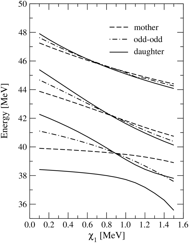
FIG. 1.: The exact energies for the states of the mother (dashed line) intermediate (dashed dot line) and daughter (full line) are plotted as function of the particle-particle interaction strength, $\chi_{1}$.

FIG. 2.: The transition amplitudes for the double beta ($2\nu\beta\beta$) Fermi transition, corresponding to the exact eigenstates and energies of the model Hamiltonian (full line) and the new QRPA approach of the present paper(dashed line), are plotted as function of $\chi_{1}$.

FIG. 3.: The transition amplitude for the double beta Fermi transition calculated within the standard $pnQRPA$, is represented as function of $\chi_{1}$.

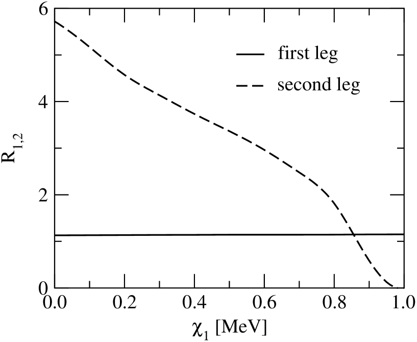
FIG. 4.: The ratio of the first single beta matrix element involved in eq (5.2) obtained within the standard pnQRPA and the present approach respectively (full line), is represented as function of $\chi_{1}$. The ratio corresponding to the second leg of the double beta transition is plotted by a dashed line.

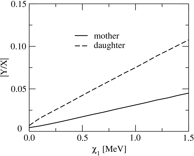
FIG. 5.: The magnitude of the ratio of the phonon amplitudes calculated within the present approach, is represented as function of $\chi_{1}$ for mother (full line) and daughter nuclei (dashed line).

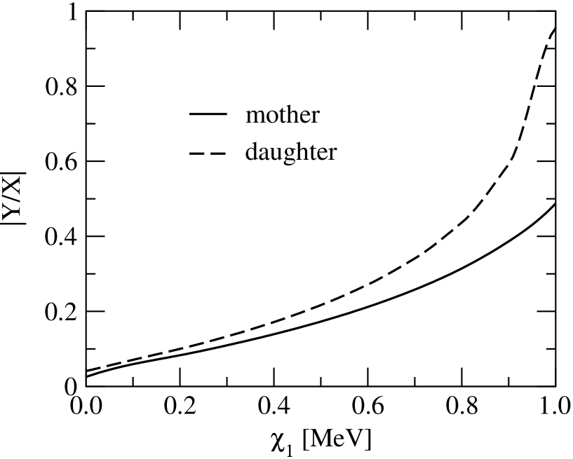
FIG. 6.: The magnitude of the ratio of the phonon amplitudes, calculated within the standard $pnQRPA$, is represented as function of $\chi_{1}$ for mother (full line) and daughter nuclei (dashed line).

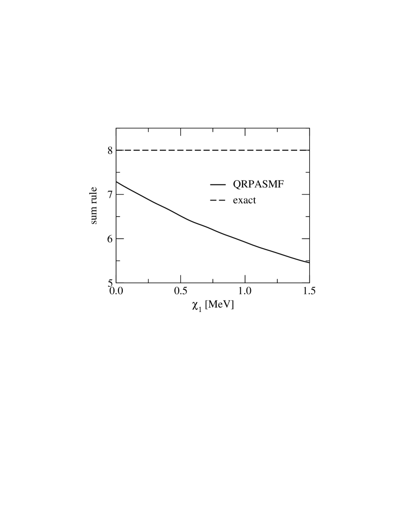
FIG. 7.: The $N-Z$ sum rule corresponding to the exact description of nuclear states(dashed line) an to the present approach, is represented as function of $\chi_{1}$.

REFERENCES

• [1] L. S. Kisslinger and R. A. Sorensen, Mat. Fys. Medd. Dan. Vid. Selsk. 32,No 16 (1960), pp. 5-82.
• [2] S. T. Belyaev, Matt. Phys. Medd. 31 (1959) 5-55.
• [3] B. F. Bayman, Nucl. Phys. 15 (1960) 33.
• [4] R. R. Chasman, Phys. Rev. 132 (1963) 343.
• [5] M. Baranger and M. Veneroni, Ann. Phys.114(1978)123
• [6] H. Toki, K. Neergard, P. Vogel and A. Faessler, Nucl. Phys. A279 (1977) 1.
• [7] I. Hamamoto, Nucl. Phys. A271 (1976) 15.
• [8] F. Grummer, K. W. Schmid and A. Faessler, Nucl. Phys. A326 (1979) 1.
• [9] A. Ikeda, N. Onishi, Prog. Theor. Phys. 70 (1983) 128.
• [10] E. Marshalek, Nucleonika 23 (1978) 409.
• [11] E. Moya de Guerra and F. Villars, Nucl. Phys. A285 (1977) 297, A298 (1978) 109.
• [12] A. A. Raduta, V. Ceausescu, A. Gheorghe and M. S. Popa, Nucl. Phys. A 427 (1984) 1.
• [13] A. Goswami, Nucl. Phys. 60 (1964) 228.
• [14] P. Camiz, A. Covello and M. Jean, Nuovo Cimento 36 (1965) 663; 42 (1966) 199.
• [15] M. Jean, Proc. Predeal Summer School, Predeal, Romania 1969.
• [16] H. H. Wolter, A. Faessler and P. U. Sauer, Phys. Lett. B 31 (1970) 516.
• [17] A. L. Goodman, Nucl. Phys. A 186 (1972) 475.
• [18] K. Langanke, D. J. Dean, S. E. Koonin and P.B. Radha, Nucl. Phys. A 613 (1997) 253.
• [19] A. L. Goodman, Adv. Nucl. Phys. 11 (1979) 263.
• [20] A. L. Goodman, Phys. Rev. C 58 (1998) R3051.
• [21] Y. Takahashi, Prog. Th. Phys., 46 (1971) 1749.
• [22] E. M. Muller, K. Muhlhaus, K. Neergard and U. Mosel, Nucl. Phys. A 383 (1982) 233.
• [23] M. Cheoun, A. Bobyk, A. Faessler, F. Symkovic and G. Teneva, Nucl. Phys. A561(1993)74, A564 (1993) 329.
• [24] J. Engel, S. Pittel, M. Stoitsov, P. Vogel and J. Dukelsky, Phys. Rev. 55 (1997) 1781.
• [25] W. Satula and R. Wyss, Phys. Lett. B 393 (1997) 1.
• [26] J. Terasaki, R. Wyss and P. H. Heenen, Phys. Lett. B 437 (1998) 1.
• [27] W.C. Haxton, G.J. Stephensen Jr., Prog. Part. Nucl. Phys. 12 (1984) 409.
• [28] A. Faessler, Prog. Part.Nucl. Phys. 21 (1988) 183.
• [29] A. Faessler and F. Simkovic J. Phys. G 24 (1998) 2139.
• [30] J. Suhonen and O. Civitarese, Phys. Rep. 300 (1998) 123.
• [31] D. Cha, Phys. Rev. C27 (1983) 2269.
• [32] P. Vogel and P. Fisher, Phys. Rev. C32 (1985) 1362.
• [33] P. Vogel and M. R. Zirnbauer, Phys. Rev. Lett. 57(1986) 3148.
• [34] O. Civitarese, A. Faessler and T. Tomoda, Phys. Lett. B194 (1986) 11.
• [35] H. V. Klapdor and K. Grotz, Phys. Lett. B 142 (1984) 323.
• [36] J. Suhonen, T. Taigel and A. Faessler,Nucl. Phys. A 486 (1988) 91.
• [37] A. A. Raduta, A. Faessler, S. Stoica and W. Kaminski Phys. Lett. B 254 (1991) 7.
• [38] A. A. Raduta, A. Faessler and S. Stoica Nucl. Phys. A 534 (1991) 149.
• [39] A. Grifiths and P. Vogel, Phys. Rev. C 46 (1992) 181.
• [40] J. Suhonen, Nucl. Phys. A 563 (1993) 205.
• [41] J. Toivanen and J. Suhonen, Phys. Rev. Lett. 75 (1995) 410.
• [42] A. A. Raduta, M. C. Raduta, A. Faessler and W. A. Kaminski, Nucl. Phys. A 634 (1998) 497.
• [43] A. A. Raduta, F. Simkovic and A. Faessler, Jour. Phys. G 26 (2000) 793.
• [44] F. Simkovic, A. A. Raduta, M. Veselsky and A. Faessler, Phys. Rev. C 61 (2000) 044319.
• [45] A.A. Raduta, O. Haug, F. Šimkovic, and A. Faessler, J. Phys. G 26 (2000) 1327; Nucl. Phys. A 671 (2000) 255.
• [46] A. A. Raduta, L. Pacearescu, V. Baran, P. Sarriguren and E. Moya de Guerra, Nucl. Phys. A 675 (2000) 503.
• [47] F. Villars, Nucl. Phys. A 285 (1977) 269.
• [48] M. Sambataro and J. Suhonen, Phys. Rev. C 56 (1997) 782.
• [49] M. K. Cheoun, A. Faessler, F. Simkovic, and G. Teneva, A. Bobyk, Nucl. Phys. A 587 (1995) 301.
Refer to caption