Remarks on the extraction of freeze-out parameters

Abstract

I review the extraction of kinetic and chemical freeze-out parameters from experimental data, with particular emphasis on the underlying assumptions and the validity of the conclusions.

1 INTRODUCTION

Collisions of elementary particles, hadrons, and nuclei at ultrarelativistic energies produce a multitude of particles (“multiparticle production”). Final-state interactions between the produced particles determine the dynamical evolution of the system. In $e^{+}e^{-}$ and hadron-hadron collisions only few particles are produced, and it is unlikely that many final-state interactions occur. The particles decouple (“freeze out”) from the system soon after production.

On the other hand, in $AA$ collisions the density of produced particles is sufficiently large over an extended region in space-time, such that the mean free path of produced particles becomes small and many final-state interactions occur. These interactions drive the system towards local thermodynamic, i.e., thermal, mechanical, and chemical equilibrium. In local thermodynamic equilibrium, the evolution of the system is governed by the equations of ideal fluid dynamics [1]. If the system is only thermally and mechanically, i.e., kinetically, but not chemically equilibrated, these equations have to be supplemented by rate equations which determine the chemical composition of the system [2]. In both cases, pressure gradients between dense, equilibrated matter and the vacuum drive collective expansion, which cools and dilutes the system. Freeze-out of particles occurs when microscopic interaction rates become smaller than the macroscopic expansion rate of the system.

By definition, after freeze-out the momenta of the produced particles do not change. The experimentally measured spectra of hadronic particles thus reflect the state of the system at freeze-out. The question is whether the spectra can also tell us about the state of the system prior to freeze-out? For instance, can they tell us whether the system was in thermodynamic, or at least kinetic equilibrium? Do they provide information as to whether a quark-gluon plasma (QGP), i.e., an equilibrated state of quarks and gluons, was created at some stage during the evolution of the system?

These questions are addressed in the following. In section 2, I discuss whether the exponential nature of single-inclusive, invariant particle spectra is sufficient to conclude that the system was in thermal equilibrium. In section 3, it is argued that in $AA$ collisions collective expansion is likely to occur prior to kinetic freeze-out. In section 4, I discuss how final-state particle ratios yield information about the thermodynamic conditions at chemical freeze-out. Conclusions are given in section 5.

2 EXPONENTIAL PARTICLE SPECTRA

In multiparticle production processes, single-inclusive, invariant particle spectra are typically exponential in the transverse momentum, $p_{T}$. The reason for the exponential behavior is the phase space of the final multiparticle state [3]. Consider for instance a process where two particles (or nuclei) collide and produce $N$ particles in the final state. Label the 4-momenta of the two incoming particles as ${p_{1}^{\prime}}^{\mu}$ and ${p_{2}^{\prime}}^{\mu}$, and the 4-momenta of the $N$ outgoing particles as $p_{1}^{\mu},\,p_{2}^{\mu},\,\ldots,\,p_{N}^{\mu}$. All 4-momenta are on-shell, $p_{i}^{\mu}\equiv(E_{i},{\bf p}_{i})$, $E_{i}\equiv\sqrt{{\bf p}_{i}^{2}+m_{i}^{2}}$. The total 4-momentum is conserved, $P^{\mu}\equiv{p_{1}^{\prime}}^{\mu}+{p_{2}^{\prime}}^{\mu}\equiv\sum_{i=1}^{N}p_{i}^{\mu}$. Up to constants depending on ${p_{1}^{\prime}}^{\mu}$ and ${p_{2}^{\prime}}^{\mu}$, the total cross section for this process is [3]

$$\sigma\sim\int\prod_{i=1}^{N}\,\frac{{\rm d}^{3}{\bf p}_{i}}{E_{i}}\;\delta^{(4)}\left(P^{\mu}-\sum_{i=1}^{N}p_{i}^{\mu}\right)\;|{\cal M}(P,p_{1},\ldots,p_{N})|^{2}\,\,,$$ (1)

where the integration is over the $3\,N$ dimensional momentum space of particles in the final state, the delta function represents energy conservation, and $|{\cal M}|^{2}$ is the modulus squared of the matrix element for the $2\rightarrow N$ process. The single-inclusive, invariant cross section for the production of a certain particle species – without loss of generality assumed to have 4-momentum $p_{1}^{\mu}$ – is then (again, up to constants)

$$E_{1}\,\frac{{\rm d}\sigma}{{\rm d}^{3}{\bf p}_{1}}\sim\int\prod_{i=2}^{N}\,\frac{{\rm d}^{3}{\bf p}_{i}}{E_{i}}\;\delta^{(4)}\left(P^{\mu}-p_{1}^{\mu}-\sum_{i=2}^{N}p_{i}^{\mu}\right)\;|{\cal M}(P,p_{1},\ldots,p_{N})|^{2}\,\,.$$ (2)

Let us introduce the “average” matrix element,

$$\left\langle|{\cal M}(P,p_{1},\ldots,p_{N})|^{2}\right\rangle_{p_{2},\ldots,p_{N}}$$ (3)

$$\equiv \left[\Phi(P-p_{1})\right]^{-1}\;\int\prod_{i=2}^{N}\,\frac{{\rm d}^{3}{\bf p}_{i}}{E_{i}}\;\delta^{(4)}\left(P^{\mu}-p_{1}^{\mu}-\sum_{i=2}^{N}p_{i}^{\mu}\right)\;|{\cal M}(P,p_{1},\ldots,p_{N})|^{2}\,\,,$$

where the average is over the $3\,(N-1)$ dimensional momentum space of the unobserved $N-1$ particles in the single-inclusive production of the particle with momentum $p_{1}$, and

$$\Phi(P-p_{1})\equiv\int\prod_{i=2}^{N}\,\frac{{\rm d}^{3}{\bf p}_{i}}{E_{i}}\;\delta^{(4)}\left(P^{\mu}-p_{1}^{\mu}-\sum_{i=2}^{N}p_{i}^{\mu}\right)$$ (4)

is the corresponding Lorentz-invariant momentum-space volume. The momentum-space volume has dimension MeV^2(N-3). Then, the single-inclusive cross section can be written as

$$E_{1}\,\frac{{\rm d}\sigma}{{\rm d}^{3}{\bf p}_{1}}\sim\Phi(P-p_{1})\;\left\langle|{\cal M}(P,p_{1},\ldots,p_{N})|^{2}\right\rangle_{p_{2},\ldots,p_{N}}\,\,.$$ (5)

Dynamical information about the $2\rightarrow N$ process is contained in the second term only. The first factor, the momentum-space volume, is in some sense trivial.

To compute the momentum-space volume, for the sake of simplicity (and because it allows us to obtain a purely analytic result) let us assume that all $N$ particles in the final state are massless. In this case, no other scale with the dimension of energy enters $\Phi(P-p_{1})$, and for dimensional reasons,

$$\Phi(P-p_{1})\sim\left[(P-p_{1})^{2}\right]^{N-3}\,\,.$$ (6)

Because $\Phi(P-p_{1})$ is Lorentz-invariant, one may evaluate the right-hand side in the C.M. frame of the incoming particles, where $P^{\mu}\equiv(E,{\bf 0})$, with the result

$$\Phi(P-p_{1})\sim E^{2(N-3)}\left(1-\frac{E_{1}}{E/2N}\,\frac{N-3}{N}\,\frac{1}{N-3}\right)^{N-3}\,\,.$$ (7)

In the limit $N\gg 1$, the term in parentheses is a representation for the exponential function, $\lim_{n\rightarrow\infty}(1+x/n)^{n}\equiv e^{x}$, such that

$$\Phi(P-p_{1})\sim\exp\left(-\frac{E_{1}}{E/2N}\right)\,\,,\;\;\;\;N\gg 1\,\,.$$ (8)

Now insert this into Eq. (5), and divide by the total cross section to obtain the invariant momentum spectrum. Then, for a given rapidity $y_{1}$, for instance $y_{1}=0$, one obtains

$$\left.\frac{{\rm d}N}{{\rm d}y_{1}\,{\rm d}^{2}{\bf p}_{T,1}}\right|_{y_{1}=0}\sim\exp\left(-\frac{p_{T,1}}{E/2N}\right)\,\,.$$ (9)

Provided that the average matrix element squared $\langle|{\cal M}|^{2}\rangle$ does not contain a strong (exponential) dependence on $p_{T,1}$, the invariant momentum spectrum decreases exponentially with $p_{T,1}$, with an inverse slope parameter $T_{\rm slope}=E/2N$, which proves our original assertion. The exponential behavior of the transverse momentum spectra is due to phase space [4]. No assumption about thermal equilibration is necessary to obtain this result.

Nevertheless, single-inclusive particle spectra are also exponential in thermal equilibrium, i.e., for a system at temperature $T$. In this case, the invariant transverse momentum spectrum is given by the Cooper-Frye formula [5]

$$E_{1}\,\frac{{\rm d}N}{{\rm d}^{3}{\bf p}_{1}}=\int_{\Sigma}{\rm d}\Sigma\cdot p_{1}\;f\left(\frac{p_{1}\cdot u}{T},\lambda_{1}\right)\,\,,$$ (10)

where $\Sigma$ is the 3-dimensional space-time hypersurface on which the transverse momentum spectrum is computed, ${\rm d}\Sigma^{\mu}$ is the normal vector on $\Sigma$, and $f(x,\lambda)$ is the thermal distribution function. For Boltzmann particles, $f(x,\lambda)\sim\lambda\,\exp(-x)$; $\lambda\equiv\exp(\mu/T)$ is the fugacity of the particle, and $\mu$ the chemical potential. The 4-vector $u^{\mu}$ in Eq. (10) is the 4-velocity of the system, i.e., the average 4-velocity of particle flow. In the rest frame of the system, $u^{\mu}\equiv(1,{\bf 0})$.

For the sake of simplicity, compute the spectrum at constant time, where ${\rm d}\Sigma^{\mu}=({\rm d}^{3}{\bf x},{\bf 0})$, such that

$$E_{1}\,\frac{{\rm d}N}{{\rm d}^{3}{\bf p}_{1}}\sim V\,\lambda_{1}\,E_{1}\,\;\exp\left(-\frac{E_{1}}{T}\right)\,\,.$$ (11)

For ultrarelativistic particles, the energy per particle is related to the temperature via $E/N=3\,T$, such that at midrapidity

$$\left.\frac{{\rm d}N}{{\rm d}y_{1}\,{\rm d}^{2}{\bf p}_{T,1}}\right|_{y_{1}=0}\sim\exp\left(-\frac{p_{T,1}}{E/3N}\right)\,\,.$$ (12)

This is rather similar to Eq. (9), except that the (inverse) slope of the $p_{T}$-spectrum is equal to the true thermodynamic temperature $T=E/3N$, while previously, $T_{\rm slope}=E/2N$ is a factor 3/2 larger.

The origin of this discrepancy is that invariant momentum space is not identical to thermodynamic momentum space. For a single particle, the former is ${\rm d}^{3}{\bf p}/E$, while the latter is ${\rm d}^{3}{\bf p}$. The missing factor of $1/E$ is responsible for the difference in the exponential slope.

From an experimental point of view, without a fully exclusive measurement one cannot precisely tell the number of particles in the final state, such that the energy per particle $E/N$ is unknown. The important point is that then there is no possibility to distinguish between the two cases Eqs. (9) and (12): usually, the strategy is to perform an exponential fit to transverse momentum spectra with a slope parameter $T_{\rm slope}$, but in this way one cannot test whether the relationship between $E/N$ and $T_{\rm slope}$ is the same as in thermal equilibrium. Although the spectra are exponential, like for a thermal system, the system need not be in thermal equilibrium. Although the slope parameter is a quantity with the same dimension as temperature, temperature is not defined, if the system is not in thermal equilibrium. One may even go one step further: although single-inclusive spectra for different particle species may have the same slope parameter, this does not mean that the system is in thermal equilibrium. It is simply due to the fact that the slope is proportional to the energy per particle $E/N$, which is a constant for all $N$ particles in the final state of a $2\rightarrow N$ process at a given C.M. energy $E$.

3 KINETIC FREEZE-OUT

Slope parameters for the most abundant particle species show different behavior as a function of particle mass in $AA$ as compared to $pp$ collisions [6]. In $AA$ collisions, they increase linearly with the particle mass,

$$T_{{\rm slope},\,AA}\simeq a+b\;m\,\,,$$ (13)

while in $pp$ collisions, they are independent of the particle mass,

$$T_{{\rm slope},\,pp}\simeq a\,\,.$$ (14)

For CERN-SPS energies, $a\simeq 140$ MeV for both $AA$ and $pp$ collisions, while $b$ depends on the system size; it increases with the mass number $A$ of the nuclei.

Although there might be other explanations for this behavior, the most natural interpretation is in terms of collective motion. The parameter $a$ is the slope parameter determined by multiparticle momentum space. Since the energy per particle $E/N$ is an intensive quantity, in both cases $a\sim E/N$ is independent of the system size. Once the particles are created, however, the environment matters, i.e., whether there are many final-state interactions, like in $AA$ collisions, or whether the particles more or less freely stream towards the detector, like in $e^{+}e^{-}$ and $pp$ collisions. As explained in the introduction, in the first case local kinetic equilibration of the system leads to pressure gradients, which in turn generate collective motion. The constant $b$ parametrizes this collective motion; it is proportional to the (average) collective flow velocity of the expanding system [7]. The larger the system, the more final-state interactions occur, and the larger is the collective flow velocity. Consequently, $b$ increases with the system size.

A word of caution is in order. The fact that there is collective motion in $AA$ collisions does not necessarily mean that local kinetic equilibrium is established and, consequently, ideal fluid dynamics applies to determine the evolution of the system. Pressure gradients which drive collective motion occur also in systems away from equilibrium. Nevertheless, the fact that there is collective motion indicates that there are final-state interactions, which will eventually drive the system towards kinetic equilibrium, unless the macroscopic expansion rate considerably exceeds the microscopic scattering rate. Therefore, the ideal-fluid approximation for the dynamical evolution of the system might not be too bad, especially for collisions of large nuclei at ultrarelativistic energies.

Freeze-out of particles occurs when microscopic interaction rates become small as compared to the macroscopic collective expansion rate. In fluid dynamical models, one commonly assumes kinetic freeze-out to happen instantaneously along space-time hypersurfaces of constant density or temperature. This is certainly an idealization: microscopically, a particle has a certain probability to decouple anywhere and anytime during the evolution of the system [8].

The invariant momentum spectra of frozen-out particles are computed according to Eq. (10), with the freeze-out hypersurface $\Sigma\equiv\Sigma_{\rm f.o.}$. There are a number of conceptual problems with this formula, a discussion of which is beyond the scope of this talk, see Refs. [9] for more details. In practice, however, the Cooper-Frye formula (10) is sufficient to compute the particle spectra to reasonable accuracy.

Let us assume that kinetic freeze-out happens across a surface of constant temperature $T_{\rm f.o.}$. Applying the mean-value theorem to Eq. (10), the spectrum of frozen-out particles at midrapidity $y=0$ is

$$\left.\frac{{\rm d}N}{{\rm d}y\,{\rm d}^{2}{\bf p}_{T}}\right|_{y=0}\sim\exp\left(-\langle\gamma\rangle\frac{m_{T}-{\bf p}_{T}\cdot\langle{\bf v}_{T}\rangle}{T_{\rm f.o.}}\right)\,\,,$$ (15)

where $\langle{\bf v}_{T}\rangle$ and $\langle\gamma\rangle$ are suitably defined average values for the transverse fluid 3-velocity and the Lorentz gamma factor along the freeze-out hypersurface. At $y=0$, it is reasonable to neglect longitudinal collective motion, such that $\gamma\simeq(1-{\bf v_{T}}^{2})^{-1/2}$ is determined by ${\bf v}_{T}$. Assuming azimuthal symmetry, the spectrum (15) then depends only on two parameters, the kinetic freeze-out temperature $T_{\rm f.o.}$ and the modulus of the average transverse collective flow velocity $\langle v_{T}\rangle$.

Table 1: Kinetic freeze-out temperatures and average transverse flow velocities for $PbPb$ collisions at $E_{\rm Lab}=158\,A$GeV.

Ref.	$T_{\rm f.o.}$ [MeV]	$\langle v_{T}\rangle$
[10]	140	0.55
[11]	110 – 120	0.60
[12]	120 – 140
[13]	130	0.50
[14]	120	0.43
[15]	100	0.55
[16]	140	0.55

Table 1 shows values for $T_{\rm f.o.}$ and $\langle v_{T}\rangle$ extracted by several authors from experimental spectra for $PbPb$ collisions at CERN-SPS energies, $E_{\rm Lab}=158\,A$GeV. From Eq. (15) it is obvious that $T_{\rm f.o.}$ and $\langle v_{T}\rangle$ are correlated: fits of similar quality can be obtained by trading off a lower value for $T_{\rm f.o.}$ against a higher value for $\langle v_{T}\rangle$ and vice versa. This can also be seen in the values quoted in Table 1. This ambiguity can be removed by two-particle correlations, where $T_{\rm f.o.}$ and $\langle v_{T}\rangle$ are correlated in the opposite way [15].

4 CHEMICAL FREEZE-OUT

In principle, there is another, independent way to determine thermodynamic quantities at freeze-out. First note that, in order to compute the transverse momentum spectrum (15) of particle species $i$, one not only needs to know the temperature and the transverse flow velocity along the freeze-out hypersurface, which determine the shape of the spectrum as a function of $p_{T}$, but also the fugacity $\lambda_{i,{\rm f.o.}}\equiv\exp(\mu_{i,{\rm f.o.}}/T_{\rm f.o.})$, which determines the absolute normalization of the spectrum, cf. Eq. (10). In general, $\mu_{i,{\rm f.o.}}$ varies along the freeze-out hypersurface, but in order to proceed, let us make the assumption (the first of three) that it is constant, like the temperature $T_{\rm f.o.}$. In the following, we shall drop the subscript “f.o.”, but remember that all thermodynamic quantities, as well as the flow 4-velocity $u^{\mu}$, are taken on the freeze-out hypersurface.

The second assumption we shall make is that all particle species freeze out across the same freeze-out hypersurface. This is certainly an idealization, as the mean free paths of different particle species are different [8]. Under these two assumptions, the ratio of the total particle numbers of particle species $i$ and $j$ is

$$\frac{N_{i}}{N_{j}}\equiv\frac{\int({\rm d}^{3}{\bf p}_{i}/E_{i})\,\int_{\Sigma}{\rm d}\Sigma\cdot p_{i}\,f(p_{i}\cdot u/T,\lambda_{i})}{\int({\rm d}^{3}{\bf p}_{j}/E_{j})\,\int_{\Sigma}{\rm d}\Sigma\cdot p_{j}\,f(p_{j}\cdot u/T,\lambda_{j})}\equiv\frac{\int_{\Sigma}{\rm d}\Sigma\cdot{\cal N}_{i}}{\int_{\Sigma}{\rm d}\Sigma\cdot{\cal N}_{j}}\,\,,$$ (16)

where

$${\cal N}_{i}^{\mu}\equiv\int\frac{{\rm d}^{3}{\bf p}_{i}}{E_{i}}\,p_{i}^{\mu}f\left(\frac{p_{i}\cdot u}{T},\lambda_{i}\right)$$ (17)

is the 4-current of particle species $i$. In kinetic equilibrium the 4-current assumes the simple form ${\cal N}_{i}^{\mu}\equiv n_{i}\,u^{\mu}$, where $n_{i}=n_{i}(T,\mu_{i})$ is the density of particles of species $i$ in the local rest frame. The flow 4-velocity $u^{\mu}$ is common to all particle species because the system is assumed to be kinetically equilibrated immediately prior to freeze-out. Equation (16) becomes [17]

$$\frac{N_{i}}{N_{j}}\equiv\frac{n_{i}(T,\mu_{i})}{n_{j}(T,\mu_{j})}\,\,,$$ (18)

because the factor $\int_{\Sigma}{\rm d}\Sigma\cdot u$ cancels between numerator and denominator. The result (18) is remarkable in the sense that, under the present assumptions, the ratio of total particle yields is independent of the detailed dynamical evolution of the system prior to freeze-out. Moreover, this ratio is the same as for a system in global kinetic equilibrium at temperature $T$ with chemical potentials $\mu_{1},\,\mu_{2},\ldots$.

Let us now make the third assumption, namely that the system is not only in kinetic, i.e., thermal and mechanical equilibrium, but also in chemical equilibrium. This assumption is fulfilled if inelastic (and not only elastic) collision rates are sufficiently large. In this case, the chemical potential of particle species $i$ is given by

$$\mu_{i}=b_{i}\;\mu_{B}+s_{i}\;\mu_{S}+e_{i}\;\mu_{e}+\ldots\,\,,$$ (19)

where $\mu_{B},\,\mu_{S},$ and $\mu_{e}$ are baryon, strangeness, and electric charge chemical potentials, respectively, and $b_{i},\,s_{i},\,e_{i}$ are baryon, strangeness, and electric charges of particle species $i$. The ellipsis in Eq. (19) stands for possible other conserved charges with associated chemical potentials.

Global baryon, strangeness, and charge conservation impose additional conditions which allow to eliminate all charge chemical potentials except for one, e.g. $\mu_{B}$. Then, all particle ratios are a function of two parameters only, $T$ and $\mu_{B}$. Taking into account the known (vacuum) values for the hadronic masses $m_{i}$ and the (vacuum) partial decay widths $\Gamma_{i\rightarrow jk\ldots}$, one can then extract $T$ and $\mu_{B}$ from ($4\pi$ extrapolated) data via a $\chi^{2}$ analysis.

Different authors use slightly different strategies to perform such $\chi^{2}$ fits. Some introduce a hard-core repulsion between hadrons [18, 19], some relax the assumption of chemical equilibration of strangeness [20, 21], some conserve strangeness exactly in the canonical ensemble [22]. In essence, all methods introduce at least one additional parameter, which of course improves the quality of the fit, but does not fundamentally change the underlying assumptions. All fits are roughly of the same quality, which makes it hard to draw definite conclusions regarding the necessity of the individual approach.

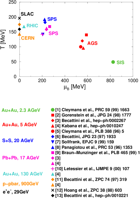
Figure 1: Values for temperature $T$ and chemical potential $\mu_{B}$ extracted from particle ratios. Different collision energies and systems are shown in different colors. Different symbols indicate differences in the fitting procedure, for more details see listed references (numbering not identical with that in main text).

Results of $\chi^{2}$ analyses for $e^{+}e^{-}$, $pp$, as well as $AA$ collisions with equal-mass nuclei at various collision energies are compiled in Fig. 1 (see also [17, 23] for a similar compilation). Two features are remarkable: first, as noted by Cleymans and Redlich [17], all $(T,\mu_{B})$ combinations fall on a line of constant energy per particle, $\langle E\rangle/\langle N\rangle\simeq 1$ GeV. The value 1 GeV can be intuitively understood as setting the energy scale below which inelastic collisions cease and therefore chemical equilibration becomes impossible.

The second feature is that, at CERN-SPS energies and above, the freeze-out temperature is $T\sim 160$ MeV, which is somewhat higher than the kinetic freeze-out temperature discussed in the last section. This can be understood rather naturally noting that the extraction of a freeze-out temperature from particle ratios assumed chemical equilibrium, while the extraction from single-inclusive spectra only assumed kinetic equilibrium. Thus, particle ratios determine the temperature at chemical freeze-out, and not at kinetic freeze-out. Since chemical equilibrium requires frequent inelastic collisions, while kinetic equilibrium only requires frequent elastic collisions, chemical freeze-out occurs earlier, i.e., at larger temperatures, than kinetic freeze-out. In order to distinguish quantities at chemical from those at kinetic freeze-out, in the following the former will be denoted with a subscript “ch.”, and the latter with the subscript “f.o.”, as above.

Given a set of hadronic masses $m_{i}$ and decay widths $\Gamma_{i\rightarrow jk\ldots}$, the extracted values of $(T,\mu_{B})_{\rm ch.}$ displayed in Fig. 1 are relatively insensitive to errors in the experimental determination of total particle numbers. This can be seen in the non-relativistic approximation,

$$n_{i}(T,\mu_{i})\sim\exp\left(\frac{\mu_{i}-m_{i}}{T}\right)\,\,,$$ (20)

such that Eq. (18) becomes

$$\frac{N_{i}}{N_{j}}\sim\exp\left(\frac{\mu_{i,{\rm ch.}}-\mu_{j,{\rm ch.}}}{T_{\rm ch.}}-\frac{m_{i}-m_{j}}{T_{\rm ch.}}\right)\,\,.$$ (21)

Errors in the determination of $N_{i}$ and $N_{j}$ influence the fitted values for $T_{\rm ch.}$ and $\mu_{B,{\rm ch.}}$ only logarithmically.

On the other hand, as can be also seen from Eq. (21), the values for the hadronic masses $m_{i}$ entering the fit influence $T_{\rm ch.}$ and $\mu_{B,{\rm ch.}}$ linearly. Most fits assume that the hadronic masses and decay widths at chemical freeze-out are the same as in vacuum. At such large temperatures and chemical potentials, however, a change of mass and decay width due to in-medium interactions cannot be excluded [24, 25, 26], $m_{i}\rightarrow m_{i}^{*},\;\Gamma_{i\rightarrow jk}\rightarrow\Gamma^{*}_{i\rightarrow jk}$. These interactions are elastic collisions which still occur at chemical freeze-out, since the system remains kinetically equilibrated. In [25], such an analysis was performed for $PbPb$ collisions at CERN-SPS energies in the framework of a chiral model. In this model, masses in general decrease at large density and temperature, such that the value for the chemical freeze-out temperature is smaller than for a fit with vacuum masses, $T_{\rm ch.}\simeq 144$ MeV. Interestingly, in the calculation of [25] it turns out to be approximately the same as the kinetic freeze-out temperature, although at kinetic freeze-out, particles have to attain their vacuum masses, due to the absence of any kind of interaction. Clearly, more work has to be done to understand and possibly refine the freeze-out picture, for instance, also to include in-medium modifications of the decay widths.

5 CONCLUSIONS

In this talk, I first discussed single-inclusive, invariant particle spectra in a $2\rightarrow N$ process. I explicitly demonstrated that the momentum space volume of the final-state particles gives rise to the exponential nature of these spectra. For the special case of massless particles, I showed that the slope of the spectra differs from the one for a thermally equilibrated system of particles, i.e., that exponential particle spectra alone are not indicative for the existence of thermal equilibrium.

I then argued that the slope characteristics for different particle species suggest collective motion in $AA$ collisions. Single-inclusive, invariant particle spectra then yield information about the average temperature $T_{\rm f.o.}$ and average collective flow velocity $\langle v_{T}\rangle$ at kinetic freeze-out.

Finally, I discussed the extraction of the chemical freeze-out parameters $T_{\rm ch.}$ and $\mu_{B,{\rm ch.}}$ from particle ratios. This analysis is based upon rather restrictive assumptions, and depends sensitively on the hadronic masses and decay widths.

Nevertheless, it is astonishing that a fit with essentially two parameters can reproduce a multitude of data with reasonably good quality. There could be several explanations. First, the state preceding chemical freeze-out is indeed in thermodynamic equilibrium. The degrees of freedom could be hadrons, but since $T_{\rm ch.}$ is close to the temperature of the confinement-deconfinement transition, it is, however, also conceivable that at some earlier stage in the evolution of the system a thermodynamically equilibrated QGP has existed [18, 27]. From thermodynamic arguments alone, however, one can never distinguish between these two possibilities: by definition, a state in thermodynamic equilibrium has no knowledge about its past.

The discussion of section 2 allows for a second explanation. Multiparticle production saturates the available phase space, such that final-state hadrons have exponential spectra with a slope that can be interpreted as a temperature, and an absolute normalization that can be interpreted as a fugacity. Although the discussion of section 2 has shown that the final state need not be thermodynamically equilibrated to have these properties, it then at least looks like hadrons are “born into thermodynamic equilibrium” [28]. In principle, the chemical composition could then immediately freeze out. In this case, no additional assumptions about an equilibrated state preceding chemical freeze-out are necessary. As seen in section 3, there certainly are elastic interactions which cause collective motion, but this could in principle happen after chemical freeze-out.

To distinguish between the first and second scenario, a more thorough understanding of multiparticle production in $AA$ collisions is necessary. The only way to achieve this is to compare $AA$ with $pp$ and $pA$ collisions. It is therefore mandatory to gather more experimental data on the latter at comparable collision energies.

Acknowledgements

I am indebted to J. Cleymans, B. Cole, K. Kajantie, R. Kuhn, K. Redlich, and E. Shuryak for discussions. Thanks go Columbia University’s Nuclear Theory Group for providing the computing facilities necessary to complete this work.

References

- [1] R.B. Clare and D. Strottman, Phys. Rept. 141 (1986) 177; D.H. Rischke, nucl-th/9809044.
- [2] P. Koch, B. Müller, J. Rafelski, Phys. Rept. 142 (1986) 167; D.M. Elliott and D.H. Rischke, Nucl. Phys. A 671 (2000) 583.
- [3] R. Hagedorn, Relativistic Kinematics, W.A. Benjamin, 1963; E. Byckling and K. Kajantie, Particle Kinematics, Wiley, 1973.
- [4] J. Hormuzdiar, G. Mahlon, S.D.H. Hsu, nucl-th/0001044.
- [5] F. Cooper, G. Frye, E. Schonberg, Phys. Rev. D 11 (1975) 192.
- [6] NA44 collaboration, I.G. Bearden et al., Phys. Rev. Lett. 78 (1997) 2080.
- [7] T. Csörgö, B. Lörstad, J. Zimanyi, Phys. Lett. B 338 (1994) 134.
- [8] S.A. Bass, these proceedings.
- [9] K.A. Bugaev, Nucl. Phys. A 606 (1996) 559; V.K. Magas et al., Nucl. Phys. A 661 (1999) 596.
- [10] B.R. Schlei, Heavy Ion Physics 5 (1997) 403.
- [11] C.M. Hung and E. Shuryak, Phys. Rev. C 57 (1998) 1891.
- [12] P. Huovinen, P.V. Ruuskanen, J. Sollfrank, Nucl. Phys. A 650 (1999) 227.
- [13] A. Dumitru and D.H. Rischke, Phys. Rev. C 59 (1999) 354.
- [14] B. Kämpfer, hep-ph/9612336.
- [15] T. Csörgö and B. Lörstad, Nucl. Phys. A 590 (1995) 465c, Phys. Rev. C 54 (1996) 1390; B. Tomasik, U.A. Wiedemann, U. Heinz, nucl-th/9907096.
- [16] A. Ster, T. Csörgö, B. Lörstad, Nucl. Phys. A 661 (1999) 419c.
- [17] J. Cleymans and K. Redlich, Phys. Rev. C 60 (1999) 054908.
- [18] P. Braun-Munzinger, J. Stachel, J.P. Wessels, N. Xu, Phys. Lett. B 344 (1995) 43; P. Braun-Munzinger, I. Heppe, J. Stachel, Phys. Lett. B 465 (1999) 15.
- [19] M.I. Gorenstein et al., J. Phys. G 24 (1998) 1777.
- [20] F. Becattini, J. Phys. G 23 (1997) 1933; F. Becattini et al., hep-ph/0002267.
- [21] J. Letessier and J. Rafelski, Int. J. Mod. Phys. E 9 (2000) 107.
- [22] J. Cleymans, H. Oeschler, K. Redlich, Phys. Rev. C 59 (1999) 1663.
- [23] J. Sollfrank, J. Phys. G 23 (1997) 1903.
- [24] G.E. Brown, M. Rho, C. Song, nucl-th/0010008.
- [25] D. Zschiesche et al., Nucl. Phys. A 681 (2001) 34.
- [26] W. Florkowski and W. Broniowski, Phys. Lett. B 477 (2000) 73; M. Michalec, W. Florkowski, W. Broniowski, nucl-th/0103029.
- [27] U. Heinz and M. Jacob, nucl-th/0002042.
- [28] R. Stock, Nucl. Phys. A 630 (1998) 535c, Phys. Lett. B 456 (1999) 277; U. Heinz, Nucl. Phys. A 661 (1999) 140c.