Determination of $\pi N$ scattering lengths from pionic hydrogen and pionic deuterium data

Abstract

The $\pi$N s-wave scattering lengths have been inferred from a joint analysis of the pionic hydrogen and the pionic deuterium x-ray data using a non-relativistic approach in which the $\pi$N interaction is simulated by a short-ranged potential. This potential is assumed to be isospin invariant and its range, the same for isospin I=3/2 and I=1/2, is regarded as a free parameter. The proposed model admits an exact solution of the pionic hydrogen bound state problem, i.e. the $\pi$N scattering lengths can be expressed analytically in terms of the range parameter and the shift ($\epsilon$) and width ($\Gamma$) of the 1s level of the pionic hydrogen. We demonstrate that for small shifts and short ranges from the exact expression one retrieves the standard range independent Deser-Trueman formula. The $\pi$d scattering length has been calculated exactly by solving the Faddeev equations and also by using a static approximation. It has been shown that the same very accurate static formula for $\pi$d scattering length can be derived (i) from a set of boundary conditions; (ii) by a reduction of Faddeev equations; and (iii) through a summation of Feynman diagrams. By imposing the requirement that the $\pi$d scattering length, resulting from Faddeev-type calculation, be in agreement with pionic deuterium data, we obtain bounds on the $\pi$N scattering lengths. The dominant source of uncertainty on the deduced values of the $\pi$N scattering lengths are the experimental errors in the pionic hydrogen data.

PACS numbers: 11.80.Jy, 13.75.Gx, 25.80.Dj, 25.80.Hp, 36.10.Gv

I Introduction

The determination of low-energy pion-nucleon ($\pi$N) parameters has been the focus of much theoretical and experimental efforts. The s-wave $\pi$N scattering lengths are of particular importance serving as testing ground for various theoretical considerations. In addition to that, their isovector combination provides input in the Goldberger-Miyazawa-Oehme [1] sum rule to be used to extract the $\pi$NN coupling constant. In recent years major advances have been made in the experimental and theoretical investigation of the $\pi$N system. With the advent of meson factories (LAMPF, PSI and TRIUMF) and the corresponding influx of the new high accuracy $\pi$N scattering data considerable progress has been achieved in the $\pi$N phase shift analyses [2, 3, 4] providing means to examine even such subtleties as isospin symmetry breaking effects [3, 5, 6] Recently, the $\pi$N scattering experiments have been complemented by high quality pionic x-ray measurements performed, both on pionic hydrogen [7, 8] and on pionic deuterium [9]. The measurements of the shifts and widths in the 1s levels in these atomic systems, resulting from strong $\pi$N interaction, allows to extract directly the corresponding scattering lengths, i.e. $a_{\pi p}$ and $a_{\pi d}$, respectively. Therefore, the new x-ray data constitute an independent source of information on the low-energy $\pi$N scattering parameters. On the theoretical side, the physical quantities bearing on the low-energy $\pi$N interaction have now become accessible to calculations [10] conducted within quantum chromodynamics (QCD). Since QCD is known to be highly non-perturbative at low energies, its low-energy implementation has been based instead on a chiral perturbation theory in which the effective Lagrangian is expanded in increasing powers of derivatives in meson fields and quark masses. This approach in practice involves a Taylor expansion in the meson four-momenta and therefore it may be expected that the lower the energy is, the more accurate are the predictions. In this context, the precise knowledge of the experimental values of the low-energy $\pi$N scattering parameters is essential for further development of the theory.

The purpose of this work is to extract the s-wave $\pi$N scattering lengths using exclusively the pionic hydrogen and pionic deuterium x-ray data. The key reason for proceeding along this route is that the low-energy regime can be thereby investigated without recourse to scattering data and there is no danger that the low-energy parameters have been largely determined by the data at high energies. Our treatment is purely phenomenological based on an isospin invariant potential model and we wish to clarify at the onset that this approach relinquishes any pretense of being a theory in favour of practicable calculational scheme. The investigation has two parts. In part one we take as our input the values of the $\pi$N scattering lengths determined previously from pionic hydrogen data and use them in a microscopic calculation of the $\pi$d scattering length. The latter has not been measured directly in a scattering experiment but may be extracted from the pionic deuterium x-ray data by applying the Deser-Trueman formula [11]. It is an empirical fact that the $\pi$N scattering lengths are small as compared with the deuteron size and it has been a common practice [12] to use the multiple scattering expansion for calculating the $\pi$d scattering length. Since this series rapidly converges, what has been confirmed by early Faddeev calculations [13, 14, 15], in the past with the poorly known $\pi$d scattering length there was little incentive to go beyond the second order (for a review, cf. [16, 17, 18]). At present, the experimental error on $\pi$d scattering length is at the level of 2% and the adequacy of the second order formula might be questionated. Strictly speaking, a truncation of the multiple scattering series can really only receive its justification when we actually quantify the magnitude of the higher-order terms to establish whether they are truly negligible. This question is examined in detail in this paper and the $\pi$d zero-energy scattering problem is solved exactly within a three-body formalism by introducing a zero-range model to simulate the $\pi$N s-wave interaction. One advantageous feature of this model is that it allows to obtain an analytic solution of the three-body problem in the static approximation. We demonstrate that the static solution can be obtained either by reduction of the Faddeev equations, or by imposing a suitable set of boundary conditions, or finally by performing a summation of Feynman diagrams. All three methods converge to the same analytic formula expressing the $\pi$d scattering length in terms of the $\pi$N scattering lengths. Static solution in coordinate space is very appealing and helps to develop an intuitive picture of how the individual $\pi$N amplitudes contribute to build up the $\pi$d scattering length. By solving numerically the Faddeev equations we show that the accuracy of the static approximation is comparable with the present experimental uncertainty on $a_{\pi d}$. In order to find out what the pionic deuterium data can teach us about the $\pi$N scattering lengths, the $\pi$d scattering lengths obtained as a solution of the Faddeev equations is compared with experiment. It turns out that the three-body calculation is in agreement with experiment only when the input $\pi$N scattering lengths belong to a relatively small subset of values that are consistent with pionic hydrogen data. The $\pi$N scattering lengths that belong to this subset simultaneously satisfy the constraints imposed by the pionic hydrogen and pionic deuterium data.

In part two of the present work we introduce explicitly a range parameter in order to examine the validity of the zero-range model. To achieve this goal it is essential to devise a simple and transparent representation of the $\pi$N interaction in which the two-body scattering problem with and without Coulomb interaction admits an analytic solution and we show that a two-channel isospin invariant separable potential lends itself to that end. Moreover, within this representation the exact bound state condition appropriate for the pionic hydrogen problem takes also an analytic form. The latter being a single complex constraint, is equivalent to two real equations that can be explicitly solved and as a result the $\pi$N scattering lengths are obtained as functions of the range parameter together with the 1s level shift and width in the pionic hydrogen. In particular, when the level shift is small as compared with the Coulomb energy and the range of the interaction is small in comparison with the Bohr radius, from the exact bound state condition we retrieve the Deser-Trueman formula (independent of the range parameter). Regarding the range as a free parameter we are able to extend the zero-range model and by varying this parameter in physically reasonable limits we find the results to be insensitive to the value of the range. The uncertainty on the $\pi$N scattering length caused by the lack of knowledge of the range is much smaller than that resulting from the experimental errors on the pionic hydrogen level shift and width.

The organization of this paper is as follows. In Sec. II we develop a zero-range model and review various derivations leading to the static solution of the $\pi$d scattering problem. The accuracy of the static solution is examined by comparing it with the solution of the Faddeev equations. We infer isoscalar and isovector $\pi$N scattering lengths that are consistent with both, pionic hydrogen and pionic deuterium data. In Sec. III we lift the zero-range limitation by introducing a finite range into our formalism. We present an exact treatment of the pionic hydrogen and we derive Deser-Trueman formula for that particular case. The $\pi$d scattering length obtained from the solution of the Faddeev equation is compared with experiment. Finally, the results are summarized in Sec. IV.

II Zero-range model

The central issue we wish to address in this section is how to construct a theoretical framework in which we can use the pionic deuterium data to gain information on the $\pi$N scattering lengths. The measurement of the shift and the width of the 1s level in pionic deuterium presents us with the value of $\pi$d scattering length $a_{\pi d}$. The latter quantity is defined as the elastic $\pi$d scattering amplitude evaluated at zero kinetic energy of the incident pion. This amplitude is necessarily complex because absorption reaction channels are open even at the very threshold. The most important of them is the $\pi^{-}d\to nn$ reaction, and to a lesser extend the radiative absorption $\pi^{-}d\to\gamma nn$ channel. In principle, there would be also the charge-exchange break-up channel $\pi^{-}d\to\pi^{0}nn$ that is open at threshold but this process is strongly suppressed by the centrifugal barrier. Indeed, with s-wave $\pi$N interaction there is no spin-flip possible so that for the two neutrons the $\mbox{}^{1}S_{0}$ state is not available, whereas the $\mbox{}^{3}S_{1}$ state is forbidden and they have to be produced in higher partial waves. On the whole, however, the absorptive effects are not large at threshold, judging from the magnitude of the imaginary part of the $\pi$d scattering length which empirically constitutes only about a quarter of the real part of $a_{\pi d}$. Strictly speaking, the absorptive processes contribute to both, the real and the imaginary part of $a_{\pi d}$ but in the following we are going to ignore the absorptive corrections to the real part of $a_{\pi d}$. Disregarding the absorptive processes, we shall concentrate our attention on a microscopic calculation of $a_{\pi d}$ and in order to be able to solve the ensuing three-body problem we introduce a potential description of the $\pi$N interaction to be used in the appropriate Faddeev equations.

In order to facilitate the discussion of the Faddeev approach, it is instructive to take the static model as our point of departure. The attractive feature of the static model is that it is much easier to develop and to compute since the final result for pion-deuteron scattering length takes the form of a single analytic formula that does not require off-shell information. Moreover, in our case the latter model also happens to be extremely good approximation to the full solution of the three-body problem. The earliest version of a static model, due to Brueckner [19], was based on the fixed scatterer concept and ignored all isospin complications. Here, we wish to make it somewhat more realistic introducing as our dynamical framework a set of appropriate boundary conditions, but on the other hand, we are prepared to content ourselves with a theory that has isospin invariant point like interactions. Labeling the pion as $1$ and the nucleons as $2$ and $3$, the boundary conditions representing the zero-range $\pi$-N interaction taking place on nucleon $i$ where $i=2,3$, may be written as

$$\lim_{x_{1}\to x_{i}}\overline{|\mathchoice{{\hbox{\boldmath$\displaystyle x$}}}{{\hbox{\boldmath$\textstyle x$}}}{{\hbox{\boldmath$\scriptstyle x$}}}{{\hbox{\boldmath$\scriptscriptstyle x$}}}_{1}-\mathchoice{{\hbox{\boldmath$\displaystyle x$}}}{{\hbox{\boldmath$\textstyle x$}}}{{\hbox{\boldmath$\scriptstyle x$}}}{{\hbox{\boldmath$\scriptscriptstyle x$}}}_{i}|\Psi(\mathchoice{{\hbox{\boldmath$\displaystyle x$}}}{{\hbox{\boldmath$\textstyle x$}}}{{\hbox{\boldmath$\scriptstyle x$}}}{{\hbox{\boldmath$\scriptscriptstyle x$}}}_{1},\mathchoice{{\hbox{\boldmath$\displaystyle x$}}}{{\hbox{\boldmath$\textstyle x$}}}{{\hbox{\boldmath$\scriptstyle x$}}}{{\hbox{\boldmath$\scriptscriptstyle x$}}}_{2},\mathchoice{{\hbox{\boldmath$\displaystyle x$}}}{{\hbox{\boldmath$\textstyle x$}}}{{\hbox{\boldmath$\scriptstyle x$}}}{{\hbox{\boldmath$\scriptscriptstyle x$}}}_{3})}=(\mu/m)(b_{0}+b_{1}\,\mathchoice{{\hbox{\boldmath$\displaystyle I$}}}{{\hbox{\boldmath$\textstyle I$}}}{{\hbox{\boldmath$\scriptstyle I$}}}{{\hbox{\boldmath$\scriptscriptstyle I$}}}\cdot\mathchoice{{\hbox{\boldmath$\displaystyle\tau$}}}{{\hbox{\boldmath$\textstyle\tau$}}}{{\hbox{\boldmath$\scriptstyle\tau$}}}{{\hbox{\boldmath$\scriptscriptstyle\tau$}}}_{i})\lim_{x_{1}\to x_{i}}\dfrac{\textstyle{\rm d}}{\textstyle{\rm d}x_{1}}\;\overline{|\mathchoice{{\hbox{\boldmath$\displaystyle x$}}}{{\hbox{\boldmath$\textstyle x$}}}{{\hbox{\boldmath$\scriptstyle x$}}}{{\hbox{\boldmath$\scriptscriptstyle x$}}}_{1}-\mathchoice{{\hbox{\boldmath$\displaystyle x$}}}{{\hbox{\boldmath$\textstyle x$}}}{{\hbox{\boldmath$\scriptstyle x$}}}{{\hbox{\boldmath$\scriptscriptstyle x$}}}_{i}|\Psi(\mathchoice{{\hbox{\boldmath$\displaystyle x$}}}{{\hbox{\boldmath$\textstyle x$}}}{{\hbox{\boldmath$\scriptstyle x$}}}{{\hbox{\boldmath$\scriptscriptstyle x$}}}_{1},\mathchoice{{\hbox{\boldmath$\displaystyle x$}}}{{\hbox{\boldmath$\textstyle x$}}}{{\hbox{\boldmath$\scriptstyle x$}}}{{\hbox{\boldmath$\scriptscriptstyle x$}}}_{2},\mathchoice{{\hbox{\boldmath$\displaystyle x$}}}{{\hbox{\boldmath$\textstyle x$}}}{{\hbox{\boldmath$\scriptstyle x$}}}{{\hbox{\boldmath$\scriptscriptstyle x$}}}_{3})}$$ (1)

where the bar denotes an average over directions $\mathchoice{{\hbox{\boldmath$\displaystyle x$}}}{{\hbox{\boldmath$\textstyle x$}}}{{\hbox{\boldmath$\scriptstyle x$}}}{{\hbox{\boldmath$\scriptscriptstyle x$}}}_{1}-\mathchoice{{\hbox{\boldmath$\displaystyle x$}}}{{\hbox{\boldmath$\textstyle x$}}}{{\hbox{\boldmath$\scriptstyle x$}}}{{\hbox{\boldmath$\scriptscriptstyle x$}}}_{i}$ what is equivalent to projecting out the s-wave component of the wave function $\Psi$, and the boundary condition (1) is to be imposed for each of the two nucleons. The vectors $\textstyle I$ and $\textstyle\tau$ are, respectively, the pion and the nucleon isospin operators, whereas $b_{0}$ and $b_{1}$ denote the isoscalar and isovector $\pi$-N scattering lengths, $\mu$ is the $\pi$-N reduced mass and $m$ is the pion mass. In the following we choose the c.m. of the two nucleons as the origin of the coordinate system, i.e. we set $\mathchoice{{\hbox{\boldmath$\displaystyle x$}}}{{\hbox{\boldmath$\textstyle x$}}}{{\hbox{\boldmath$\scriptstyle x$}}}{{\hbox{\boldmath$\scriptscriptstyle x$}}}_{2}=\textstyle{\frac{1}{2}}\mathchoice{{\hbox{\boldmath$\displaystyle r$}}}{{\hbox{\boldmath$\textstyle r$}}}{{\hbox{\boldmath$\scriptstyle r$}}}{{\hbox{\boldmath$\scriptscriptstyle r$}}}$ and $\mathchoice{{\hbox{\boldmath$\displaystyle x$}}}{{\hbox{\boldmath$\textstyle x$}}}{{\hbox{\boldmath$\scriptstyle x$}}}{{\hbox{\boldmath$\scriptscriptstyle x$}}}_{3}=-\textstyle{\frac{1}{2}}\mathchoice{{\hbox{\boldmath$\displaystyle r$}}}{{\hbox{\boldmath$\textstyle r$}}}{{\hbox{\boldmath$\scriptstyle r$}}}{{\hbox{\boldmath$\scriptscriptstyle r$}}}$ with $\textstyle r$ being the nucleon-nucleon separation vector. The pion vector in this Jacobi coordinate system will be denoted as $\textstyle\rho$. When the wave function $\Psi(\mathchoice{{\hbox{\boldmath$\displaystyle r$}}}{{\hbox{\boldmath$\textstyle r$}}}{{\hbox{\boldmath$\scriptstyle r$}}}{{\hbox{\boldmath$\scriptscriptstyle r$}}},\mathchoice{{\hbox{\boldmath$\displaystyle\rho$}}}{{\hbox{\boldmath$\textstyle\rho$}}}{{\hbox{\boldmath$\scriptstyle\rho$}}}{{\hbox{\boldmath$\scriptscriptstyle\rho$}}})$ describing the $\pi$NN system for the case of $\pi^{-}$ scattered off the deuteron is known, the amplitude leading to the final state with asymptotic wave function $\Phi_{f}$ is $-\left\langle\Phi_{f}|V|\Psi\right\rangle$ where $V$ denotes the potentials that have been taken out in the derivation of $\Phi_{f}$. For elastic scattering $\Phi_{f}(\mathchoice{{\hbox{\boldmath$\displaystyle\rho$}}}{{\hbox{\boldmath$\textstyle\rho$}}}{{\hbox{\boldmath$\scriptstyle\rho$}}}{{\hbox{\boldmath$\scriptscriptstyle\rho$}}},\mathchoice{{\hbox{\boldmath$\displaystyle r$}}}{{\hbox{\boldmath$\textstyle r$}}}{{\hbox{\boldmath$\scriptstyle r$}}}{{\hbox{\boldmath$\scriptscriptstyle r$}}})=\exp{(\imath\mathchoice{{\hbox{\boldmath$\displaystyle p$}}}{{\hbox{\boldmath$\textstyle p$}}}{{\hbox{\boldmath$\scriptstyle p$}}}{{\hbox{\boldmath$\scriptscriptstyle p$}}}^{\prime}\cdot\mathchoice{{\hbox{\boldmath$\displaystyle\rho$}}}{{\hbox{\boldmath$\textstyle\rho$}}}{{\hbox{\boldmath$\scriptstyle\rho$}}}{{\hbox{\boldmath$\scriptscriptstyle\rho$}}})}\,\psi_{d}(\mathchoice{{\hbox{\boldmath$\displaystyle r$}}}{{\hbox{\boldmath$\textstyle r$}}}{{\hbox{\boldmath$\scriptstyle r$}}}{{\hbox{\boldmath$\scriptscriptstyle r$}}})$ where $\mathchoice{{\hbox{\boldmath$\displaystyle p$}}}{{\hbox{\boldmath$\textstyle p$}}}{{\hbox{\boldmath$\scriptstyle p$}}}{{\hbox{\boldmath$\scriptscriptstyle p$}}}^{\prime}$ is the momentum of the outgoing pion, $\psi_{d}$ is the deuteron wave function and $V$ is the sum of the two $\pi$N potentials as asymptotically there is no $\pi$-deuteron interaction. Although in our formalism we never needed $\pi$N potentials and the $\pi$N interaction is represented by the boundary condition (1), it is in fact possible to give a formal expression for such potential (cf. [20]) and for the operator $V$ we take

$$V\Psi(\mathchoice{{\hbox{\boldmath$\displaystyle\rho$}}}{{\hbox{\boldmath$\textstyle\rho$}}}{{\hbox{\boldmath$\scriptstyle\rho$}}}{{\hbox{\boldmath$\scriptscriptstyle\rho$}}},\mathchoice{{\hbox{\boldmath$\displaystyle r$}}}{{\hbox{\boldmath$\textstyle r$}}}{{\hbox{\boldmath$\scriptstyle r$}}}{{\hbox{\boldmath$\scriptscriptstyle r$}}})=-\frac{2\pi}{\mu}\left\{(b_{0}+b_{1}\,\mathchoice{{\hbox{\boldmath$\displaystyle I$}}}{{\hbox{\boldmath$\textstyle I$}}}{{\hbox{\boldmath$\scriptstyle I$}}}{{\hbox{\boldmath$\scriptscriptstyle I$}}}\cdot\mathchoice{{\hbox{\boldmath$\displaystyle\tau$}}}{{\hbox{\boldmath$\textstyle\tau$}}}{{\hbox{\boldmath$\scriptstyle\tau$}}}{{\hbox{\boldmath$\scriptscriptstyle\tau$}}}_{2})\,\delta(\mathchoice{{\hbox{\boldmath$\displaystyle\rho$}}}{{\hbox{\boldmath$\textstyle\rho$}}}{{\hbox{\boldmath$\scriptstyle\rho$}}}{{\hbox{\boldmath$\scriptscriptstyle\rho$}}}-\textstyle{\frac{1}{2}}\mathchoice{{\hbox{\boldmath$\displaystyle r$}}}{{\hbox{\boldmath$\textstyle r$}}}{{\hbox{\boldmath$\scriptstyle r$}}}{{\hbox{\boldmath$\scriptscriptstyle r$}}})\dfrac{\textstyle{\rm d}}{\textstyle{\rm d}\rho}|\mathchoice{{\hbox{\boldmath$\displaystyle\rho$}}}{{\hbox{\boldmath$\textstyle\rho$}}}{{\hbox{\boldmath$\scriptstyle\rho$}}}{{\hbox{\boldmath$\scriptscriptstyle\rho$}}}-\textstyle{\frac{1}{2}}\mathchoice{{\hbox{\boldmath$\displaystyle r$}}}{{\hbox{\boldmath$\textstyle r$}}}{{\hbox{\boldmath$\scriptstyle r$}}}{{\hbox{\boldmath$\scriptscriptstyle r$}}}|+(b_{0}+b_{1}\,\mathchoice{{\hbox{\boldmath$\displaystyle I$}}}{{\hbox{\boldmath$\textstyle I$}}}{{\hbox{\boldmath$\scriptstyle I$}}}{{\hbox{\boldmath$\scriptscriptstyle I$}}}\cdot\mathchoice{{\hbox{\boldmath$\displaystyle\tau$}}}{{\hbox{\boldmath$\textstyle\tau$}}}{{\hbox{\boldmath$\scriptstyle\tau$}}}{{\hbox{\boldmath$\scriptscriptstyle\tau$}}}_{3})\,\delta(\mathchoice{{\hbox{\boldmath$\displaystyle\rho$}}}{{\hbox{\boldmath$\textstyle\rho$}}}{{\hbox{\boldmath$\scriptstyle\rho$}}}{{\hbox{\boldmath$\scriptscriptstyle\rho$}}}+\textstyle{\frac{1}{2}}\mathchoice{{\hbox{\boldmath$\displaystyle r$}}}{{\hbox{\boldmath$\textstyle r$}}}{{\hbox{\boldmath$\scriptstyle r$}}}{{\hbox{\boldmath$\scriptscriptstyle r$}}})\dfrac{\textstyle{\rm d}}{\textstyle{\rm d}\rho}|\mathchoice{{\hbox{\boldmath$\displaystyle\rho$}}}{{\hbox{\boldmath$\textstyle\rho$}}}{{\hbox{\boldmath$\scriptstyle\rho$}}}{{\hbox{\boldmath$\scriptscriptstyle\rho$}}}+\textstyle{\frac{1}{2}}\mathchoice{{\hbox{\boldmath$\displaystyle r$}}}{{\hbox{\boldmath$\textstyle r$}}}{{\hbox{\boldmath$\scriptstyle r$}}}{{\hbox{\boldmath$\scriptscriptstyle r$}}}|\right\}\Psi(\mathchoice{{\hbox{\boldmath$\displaystyle\rho$}}}{{\hbox{\boldmath$\textstyle\rho$}}}{{\hbox{\boldmath$\scriptstyle\rho$}}}{{\hbox{\boldmath$\scriptscriptstyle\rho$}}},\mathchoice{{\hbox{\boldmath$\displaystyle r$}}}{{\hbox{\boldmath$\textstyle r$}}}{{\hbox{\boldmath$\scriptstyle r$}}}{{\hbox{\boldmath$\scriptscriptstyle r$}}}).$$ (2)

Denoting the incident pion momentum as $\textstyle p$ and making use of the boundary conditions (1) in (2), the $\pi$-d elastic scattering amplitude $f(\mathchoice{{\hbox{\boldmath$\displaystyle p$}}}{{\hbox{\boldmath$\textstyle p$}}}{{\hbox{\boldmath$\scriptstyle p$}}}{{\hbox{\boldmath$\scriptscriptstyle p$}}}^{\prime},\mathchoice{{\hbox{\boldmath$\displaystyle p$}}}{{\hbox{\boldmath$\textstyle p$}}}{{\hbox{\boldmath$\scriptstyle p$}}}{{\hbox{\boldmath$\scriptscriptstyle p$}}})$ takes the form

$$f(\mathchoice{{\hbox{\boldmath$\displaystyle p$}}}{{\hbox{\boldmath$\textstyle p$}}}{{\hbox{\boldmath$\scriptstyle p$}}}{{\hbox{\boldmath$\scriptscriptstyle p$}}}^{\prime},\mathchoice{{\hbox{\boldmath$\displaystyle p$}}}{{\hbox{\boldmath$\textstyle p$}}}{{\hbox{\boldmath$\scriptstyle p$}}}{{\hbox{\boldmath$\scriptscriptstyle p$}}})=\frac{\nu}{m}\int\textstyle{\rm e}^{-\imath\,\mathchoice{{\hbox{\boldmath$\displaystyle p$}}}{{\hbox{\boldmath$\textstyle p$}}}{{\hbox{\boldmath$\scriptstyle p$}}}{{\hbox{\boldmath$\scriptscriptstyle p$}}}^{\prime}\cdot\mathchoice{{\hbox{\boldmath$\displaystyle\rho$}}}{{\hbox{\boldmath$\textstyle\rho$}}}{{\hbox{\boldmath$\scriptstyle\rho$}}}{{\hbox{\boldmath$\scriptscriptstyle\rho$}}}}\;\psi_{d}^{\dagger}(\mathchoice{{\hbox{\boldmath$\displaystyle r$}}}{{\hbox{\boldmath$\textstyle r$}}}{{\hbox{\boldmath$\scriptstyle r$}}}{{\hbox{\boldmath$\scriptscriptstyle r$}}})\;\left\{\delta(\mathchoice{{\hbox{\boldmath$\displaystyle\rho$}}}{{\hbox{\boldmath$\textstyle\rho$}}}{{\hbox{\boldmath$\scriptstyle\rho$}}}{{\hbox{\boldmath$\scriptscriptstyle\rho$}}}-\textstyle{\frac{1}{2}}\mathchoice{{\hbox{\boldmath$\displaystyle r$}}}{{\hbox{\boldmath$\textstyle r$}}}{{\hbox{\boldmath$\scriptstyle r$}}}{{\hbox{\boldmath$\scriptscriptstyle r$}}})|\mathchoice{{\hbox{\boldmath$\displaystyle\rho$}}}{{\hbox{\boldmath$\textstyle\rho$}}}{{\hbox{\boldmath$\scriptstyle\rho$}}}{{\hbox{\boldmath$\scriptscriptstyle\rho$}}}-\textstyle{\frac{1}{2}}\mathchoice{{\hbox{\boldmath$\displaystyle r$}}}{{\hbox{\boldmath$\textstyle r$}}}{{\hbox{\boldmath$\scriptstyle r$}}}{{\hbox{\boldmath$\scriptscriptstyle r$}}}|+\delta(\mathchoice{{\hbox{\boldmath$\displaystyle\rho$}}}{{\hbox{\boldmath$\textstyle\rho$}}}{{\hbox{\boldmath$\scriptstyle\rho$}}}{{\hbox{\boldmath$\scriptscriptstyle\rho$}}}+\textstyle{\frac{1}{2}}\mathchoice{{\hbox{\boldmath$\displaystyle r$}}}{{\hbox{\boldmath$\textstyle r$}}}{{\hbox{\boldmath$\scriptstyle r$}}}{{\hbox{\boldmath$\scriptscriptstyle r$}}})|\mathchoice{{\hbox{\boldmath$\displaystyle\rho$}}}{{\hbox{\boldmath$\textstyle\rho$}}}{{\hbox{\boldmath$\scriptstyle\rho$}}}{{\hbox{\boldmath$\scriptscriptstyle\rho$}}}+\textstyle{\frac{1}{2}}\mathchoice{{\hbox{\boldmath$\displaystyle r$}}}{{\hbox{\boldmath$\textstyle r$}}}{{\hbox{\boldmath$\scriptstyle r$}}}{{\hbox{\boldmath$\scriptscriptstyle r$}}}|\right\}\Psi(\mathchoice{{\hbox{\boldmath$\displaystyle\rho$}}}{{\hbox{\boldmath$\textstyle\rho$}}}{{\hbox{\boldmath$\scriptstyle\rho$}}}{{\hbox{\boldmath$\scriptscriptstyle\rho$}}},\mathchoice{{\hbox{\boldmath$\displaystyle r$}}}{{\hbox{\boldmath$\textstyle r$}}}{{\hbox{\boldmath$\scriptstyle r$}}}{{\hbox{\boldmath$\scriptscriptstyle r$}}})\textstyle{\rm d}^{3}\rho\;\textstyle{\rm d}^{3}r,$$ (3)

where $\nu$ is $\pi$-d reduced mass. Given the elastic $\pi$-d scattering amplitude (3), the $\pi$-d scattering length follows immediately from

$$a_{\pi d}=f(0,0).$$ (4)

With the $\pi$-N interaction assumed to be isospin invariant, it will be convenient for us to adopt an isospin notation. For the initial $\pi^{-}$-d system, the isotopic spin wave function has the form

$$\chi_{a}=\pi^{-}\tfrac{1}{\sqrt{2}}(p_{2}n_{3}-n_{2}p_{3}),$$ (5)

where the symbols $p,n,\pi^{-}$ in (5) stand for the isospin wave functions of the corresponding particles. The wave function (5) is antisymmetric in the nucleon labels, as appropriate for the state where the isospin of the two-nucleon subsystem $I_{23}$ equals zero. As a result of the interaction, the two nucleons can undergo a transition to a symmetric configuration corresponding to $I_{23}=1$ and we shall need also a function that is symmetric under two-nucleon permutation

$$\chi_{s}=\tfrac{1}{2}\pi^{-}(p_{2}n_{3}+n_{2}p_{3})-\tfrac{1}{\sqrt{2}}\pi^{0}n_{2}n_{3}.$$ (6)

Since our interest here is confined to s-wave interactions, no spin flip is possible and therefore the spin part of the wave function does not change. Regarding the nucleons as fixed scattering centers, we may anticipate that the wave function $\Psi(\mathchoice{{\hbox{\boldmath$\displaystyle\rho$}}}{{\hbox{\boldmath$\textstyle\rho$}}}{{\hbox{\boldmath$\scriptstyle\rho$}}}{{\hbox{\boldmath$\scriptscriptstyle\rho$}}},\mathchoice{{\hbox{\boldmath$\displaystyle r$}}}{{\hbox{\boldmath$\textstyle r$}}}{{\hbox{\boldmath$\scriptstyle r$}}}{{\hbox{\boldmath$\scriptscriptstyle r$}}})$ for the full system of the target nucleons and the meson will take the approximate form

$$\Psi(\mathchoice{{\hbox{\boldmath$\displaystyle\rho$}}}{{\hbox{\boldmath$\textstyle\rho$}}}{{\hbox{\boldmath$\scriptstyle\rho$}}}{{\hbox{\boldmath$\scriptscriptstyle\rho$}}},\mathchoice{{\hbox{\boldmath$\displaystyle r$}}}{{\hbox{\boldmath$\textstyle r$}}}{{\hbox{\boldmath$\scriptstyle r$}}}{{\hbox{\boldmath$\scriptscriptstyle r$}}})=e^{\imath\mathchoice{{\hbox{\boldmath$\displaystyle p$}}}{{\hbox{\boldmath$\textstyle p$}}}{{\hbox{\boldmath$\scriptstyle p$}}}{{\hbox{\boldmath$\scriptscriptstyle p$}}}\cdot\mathchoice{{\hbox{\boldmath$\displaystyle\rho$}}}{{\hbox{\boldmath$\textstyle\rho$}}}{{\hbox{\boldmath$\scriptstyle\rho$}}}{{\hbox{\boldmath$\scriptscriptstyle\rho$}}}}\,u_{d}(r)\,\chi_{a}+A(\mathchoice{{\hbox{\boldmath$\displaystyle r$}}}{{\hbox{\boldmath$\textstyle r$}}}{{\hbox{\boldmath$\scriptstyle r$}}}{{\hbox{\boldmath$\scriptscriptstyle r$}}})\left[\dfrac{\exp{(\imath p|\mathchoice{{\hbox{\boldmath$\displaystyle\rho$}}}{{\hbox{\boldmath$\textstyle\rho$}}}{{\hbox{\boldmath$\scriptstyle\rho$}}}{{\hbox{\boldmath$\scriptscriptstyle\rho$}}}-\textstyle{\frac{1}{2}}\mathchoice{{\hbox{\boldmath$\displaystyle r$}}}{{\hbox{\boldmath$\textstyle r$}}}{{\hbox{\boldmath$\scriptstyle r$}}}{{\hbox{\boldmath$\scriptscriptstyle r$}}}|)}}{|\mathchoice{{\hbox{\boldmath$\displaystyle\rho$}}}{{\hbox{\boldmath$\textstyle\rho$}}}{{\hbox{\boldmath$\scriptstyle\rho$}}}{{\hbox{\boldmath$\scriptscriptstyle\rho$}}}-\textstyle{\frac{1}{2}}\mathchoice{{\hbox{\boldmath$\displaystyle r$}}}{{\hbox{\boldmath$\textstyle r$}}}{{\hbox{\boldmath$\scriptstyle r$}}}{{\hbox{\boldmath$\scriptscriptstyle r$}}}|}+\dfrac{\exp{(\imath p|\mathchoice{{\hbox{\boldmath$\displaystyle\rho$}}}{{\hbox{\boldmath$\textstyle\rho$}}}{{\hbox{\boldmath$\scriptstyle\rho$}}}{{\hbox{\boldmath$\scriptscriptstyle\rho$}}}+\textstyle{\frac{1}{2}}\mathchoice{{\hbox{\boldmath$\displaystyle r$}}}{{\hbox{\boldmath$\textstyle r$}}}{{\hbox{\boldmath$\scriptstyle r$}}}{{\hbox{\boldmath$\scriptscriptstyle r$}}}|)}}{|\mathchoice{{\hbox{\boldmath$\displaystyle\rho$}}}{{\hbox{\boldmath$\textstyle\rho$}}}{{\hbox{\boldmath$\scriptstyle\rho$}}}{{\hbox{\boldmath$\scriptscriptstyle\rho$}}}+\textstyle{\frac{1}{2}}\mathchoice{{\hbox{\boldmath$\displaystyle r$}}}{{\hbox{\boldmath$\textstyle r$}}}{{\hbox{\boldmath$\scriptstyle r$}}}{{\hbox{\boldmath$\scriptscriptstyle r$}}}|}\right]\chi_{a}+$$ (7)

$$\mbox{}+X(\mathchoice{{\hbox{\boldmath$\displaystyle r$}}}{{\hbox{\boldmath$\textstyle r$}}}{{\hbox{\boldmath$\scriptstyle r$}}}{{\hbox{\boldmath$\scriptscriptstyle r$}}})\left[\dfrac{\exp{(\imath p|\mathchoice{{\hbox{\boldmath$\displaystyle\rho$}}}{{\hbox{\boldmath$\textstyle\rho$}}}{{\hbox{\boldmath$\scriptstyle\rho$}}}{{\hbox{\boldmath$\scriptscriptstyle\rho$}}}-\textstyle{\frac{1}{2}}\mathchoice{{\hbox{\boldmath$\displaystyle r$}}}{{\hbox{\boldmath$\textstyle r$}}}{{\hbox{\boldmath$\scriptstyle r$}}}{{\hbox{\boldmath$\scriptscriptstyle r$}}}|)}}{|\mathchoice{{\hbox{\boldmath$\displaystyle\rho$}}}{{\hbox{\boldmath$\textstyle\rho$}}}{{\hbox{\boldmath$\scriptstyle\rho$}}}{{\hbox{\boldmath$\scriptscriptstyle\rho$}}}-\textstyle{\frac{1}{2}}\mathchoice{{\hbox{\boldmath$\displaystyle r$}}}{{\hbox{\boldmath$\textstyle r$}}}{{\hbox{\boldmath$\scriptstyle r$}}}{{\hbox{\boldmath$\scriptscriptstyle r$}}}|}-\dfrac{\exp{(\imath p|\mathchoice{{\hbox{\boldmath$\displaystyle\rho$}}}{{\hbox{\boldmath$\textstyle\rho$}}}{{\hbox{\boldmath$\scriptstyle\rho$}}}{{\hbox{\boldmath$\scriptscriptstyle\rho$}}}+\textstyle{\frac{1}{2}}\mathchoice{{\hbox{\boldmath$\displaystyle r$}}}{{\hbox{\boldmath$\textstyle r$}}}{{\hbox{\boldmath$\scriptstyle r$}}}{{\hbox{\boldmath$\scriptscriptstyle r$}}}|)}}{|\mathchoice{{\hbox{\boldmath$\displaystyle\rho$}}}{{\hbox{\boldmath$\textstyle\rho$}}}{{\hbox{\boldmath$\scriptstyle\rho$}}}{{\hbox{\boldmath$\scriptscriptstyle\rho$}}}+\textstyle{\frac{1}{2}}\mathchoice{{\hbox{\boldmath$\displaystyle r$}}}{{\hbox{\boldmath$\textstyle r$}}}{{\hbox{\boldmath$\scriptstyle r$}}}{{\hbox{\boldmath$\scriptscriptstyle r$}}}|}\right]\chi_{s},\hskip 28.45274pt$$ (8)

where $u_{d}$ is the spatial part of deuteron wave function that includes also the deuteron spin and in particular may contain also the D-component. The projectile enters with momentum $\textstyle p$ and in the initial asymptotic region the pion and the target have separate wave functions (a plane wave and $u_{d}(r)$, respectively) and the propagation from one scattering center to another is described by a superposition of spherical waves. The hitherto unknown amplitudes denoted in (8), respectively, as $A(\mathchoice{{\hbox{\boldmath$\displaystyle r$}}}{{\hbox{\boldmath$\textstyle r$}}}{{\hbox{\boldmath$\scriptstyle r$}}}{{\hbox{\boldmath$\scriptscriptstyle r$}}})$ and $X(\mathchoice{{\hbox{\boldmath$\displaystyle r$}}}{{\hbox{\boldmath$\textstyle r$}}}{{\hbox{\boldmath$\scriptstyle r$}}}{{\hbox{\boldmath$\scriptscriptstyle r$}}})$ multiplying these outgoing waves emitted by the two centers account for the multiple scattering phenomena. They will be determined from the boundary conditions (1). To satisfy Pauli principle the wave function (8) must be antisymmetric in the two nucleon variables. This implies that we have to stipulate that the coefficients $A(\mathchoice{{\hbox{\boldmath$\displaystyle r$}}}{{\hbox{\boldmath$\textstyle r$}}}{{\hbox{\boldmath$\scriptstyle r$}}}{{\hbox{\boldmath$\scriptscriptstyle r$}}})$ and $X(\mathchoice{{\hbox{\boldmath$\displaystyle r$}}}{{\hbox{\boldmath$\textstyle r$}}}{{\hbox{\boldmath$\scriptstyle r$}}}{{\hbox{\boldmath$\scriptscriptstyle r$}}})$ are even under permutation of the nucleons, i.e. they must be invariant under the reflections $\mathchoice{{\hbox{\boldmath$\displaystyle r$}}}{{\hbox{\boldmath$\textstyle r$}}}{{\hbox{\boldmath$\scriptstyle r$}}}{{\hbox{\boldmath$\scriptscriptstyle r$}}}\to-\mathchoice{{\hbox{\boldmath$\displaystyle r$}}}{{\hbox{\boldmath$\textstyle r$}}}{{\hbox{\boldmath$\scriptstyle r$}}}{{\hbox{\boldmath$\scriptscriptstyle r$}}}$. For zero-energy scattering considered in this work, however, this is always the case because $A(r)$ and $X(r)$ depend then only upon the magnitude of $\textstyle r$. It is worth noting that the wave function (8) includes explicitly virtual charge exchange amplitude $X(r)$. Since our interest here is confined to zero-energy scattering, in the following we take $p=0$ in (8). Equations for the functions $A(r)$ and $X(r)$ may be obtained by substituting (8) in (1) for $i=2$ and equating the coefficients multiplying the same isospin functions. With two different isospin functions we obtain two equations and this procedure determines uniquely $A(r)$ and $X(r)$. Owing to the proper antisymmetrization of our wave function the boundary condition for $i=3$ will be then automatically satisfied. The equations obtained from (1) are

$$A(r) = \tilde{b}_{0}u_{d}(r)+(\tilde{b}_{0}/r)\,A(r)+\sqrt{2}(\tilde{b}_{1}/r)\,X(r),$$ (9a)

$$-X(r) = \sqrt{2}\tilde{b}_{1}u_{d}(r)+\sqrt{2}(\tilde{b}_{1}/r)\,A(r)+(\tilde{b}_{0}+\tilde{b}_{1})/r\,X(r).$$ (9b)

In (9) we introduced the abbreviation $\tilde{b}_{j}=(1+m/M)b_{j}$ where $M$ is the nucleon mass. The $\pi$-d scattering length is given by the overlap integral

$$a_{\pi d}=(2\nu/m)\,\int u_{d}(r)^{\dagger}A(r)\,\textstyle{\rm d}^{3}r$$ (10)

where $A(r)$ is the solution of (9)

$$A(r)=\frac{\tilde{b}_{0}+(\tilde{b}_{0}+\tilde{b}_{1})(\tilde{b}_{0}-2\tilde{b}_{1})/r}{1-\tilde{b}_{1}/r-(\tilde{b}_{0}+\tilde{b}_{1})(\tilde{b}_{0}-2\tilde{b}_{1})/r^{2}}\;u_{d}(r).$$ (11)

Using (11) in (10) and expanding $A(r)$ in powers of the $\pi$N scattering lengths, we retrieve the well known second order formula for the $\pi$-d scattering length (cf. [18])

$$a_{\pi d}^{(2)}=\frac{2\nu}{m}\left[\tilde{b}_{0}+(\tilde{b}_{0}^{2}-2\,\tilde{b}_{1}^{2})\left\langle\frac{1}{r}\right\rangle\right],$$ (12)

where the expectation value is taken with respect to the deuteron wave function. As advertised at the beginning of this section, formula (11) provides a complete solution of the problem. To examine the accuracy of the static formula we have to compare it with the exact solution of the three-body problem. The latter will be obtained by solving the Faddeev equations on which we now embark.

To solve the Faddeev equations it will be convenient for us to work in momentum space. Introducing the Faddeev partitions, we write the three-body wave function as

$$\Psi=\psi^{(1)}(\mathchoice{{\hbox{\boldmath$\displaystyle q$}}}{{\hbox{\boldmath$\textstyle q$}}}{{\hbox{\boldmath$\scriptstyle q$}}}{{\hbox{\boldmath$\scriptscriptstyle q$}}}_{1},\mathchoice{{\hbox{\boldmath$\displaystyle k$}}}{{\hbox{\boldmath$\textstyle k$}}}{{\hbox{\boldmath$\scriptstyle k$}}}{{\hbox{\boldmath$\scriptscriptstyle k$}}}_{1})+\psi^{(2)}(\mathchoice{{\hbox{\boldmath$\displaystyle q$}}}{{\hbox{\boldmath$\textstyle q$}}}{{\hbox{\boldmath$\scriptstyle q$}}}{{\hbox{\boldmath$\scriptscriptstyle q$}}}_{2},\mathchoice{{\hbox{\boldmath$\displaystyle k$}}}{{\hbox{\boldmath$\textstyle k$}}}{{\hbox{\boldmath$\scriptstyle k$}}}{{\hbox{\boldmath$\scriptscriptstyle k$}}}_{2})+\psi^{(3)}(\mathchoice{{\hbox{\boldmath$\displaystyle q$}}}{{\hbox{\boldmath$\textstyle q$}}}{{\hbox{\boldmath$\scriptstyle q$}}}{{\hbox{\boldmath$\scriptscriptstyle q$}}}_{3},\mathchoice{{\hbox{\boldmath$\displaystyle k$}}}{{\hbox{\boldmath$\textstyle k$}}}{{\hbox{\boldmath$\scriptstyle k$}}}{{\hbox{\boldmath$\scriptscriptstyle k$}}}_{3}),$$ (13)

where $\mathchoice{{\hbox{\boldmath$\displaystyle q$}}}{{\hbox{\boldmath$\textstyle q$}}}{{\hbox{\boldmath$\scriptstyle q$}}}{{\hbox{\boldmath$\scriptscriptstyle q$}}}_{1}$ denotes the relative momentum of the (23) pair whereas $\mathchoice{{\hbox{\boldmath$\displaystyle k$}}}{{\hbox{\boldmath$\textstyle k$}}}{{\hbox{\boldmath$\scriptstyle k$}}}{{\hbox{\boldmath$\scriptscriptstyle k$}}}_{1}$ is the c.m. momentum of particle 1 and cyclic permutations are implied. To obtain Faddeev equations for the amplitudes, the different partitions are written as (cf. [13])

$$\psi^{(1)}(\mathchoice{{\hbox{\boldmath$\displaystyle q$}}}{{\hbox{\boldmath$\textstyle q$}}}{{\hbox{\boldmath$\scriptstyle q$}}}{{\hbox{\boldmath$\scriptscriptstyle q$}}},\mathchoice{{\hbox{\boldmath$\displaystyle k$}}}{{\hbox{\boldmath$\textstyle k$}}}{{\hbox{\boldmath$\scriptstyle k$}}}{{\hbox{\boldmath$\scriptscriptstyle k$}}}) = (2\pi)^{3}\phi(\mathchoice{{\hbox{\boldmath$\displaystyle q$}}}{{\hbox{\boldmath$\textstyle q$}}}{{\hbox{\boldmath$\scriptstyle q$}}}{{\hbox{\boldmath$\scriptscriptstyle q$}}})\delta(\mathchoice{{\hbox{\boldmath$\displaystyle k$}}}{{\hbox{\boldmath$\textstyle k$}}}{{\hbox{\boldmath$\scriptstyle k$}}}{{\hbox{\boldmath$\scriptscriptstyle k$}}}-\mathchoice{{\hbox{\boldmath$\displaystyle p$}}}{{\hbox{\boldmath$\textstyle p$}}}{{\hbox{\boldmath$\scriptstyle p$}}}{{\hbox{\boldmath$\scriptscriptstyle p$}}})\chi_{a}+[F(\mathchoice{{\hbox{\boldmath$\displaystyle q$}}}{{\hbox{\boldmath$\textstyle q$}}}{{\hbox{\boldmath$\scriptstyle q$}}}{{\hbox{\boldmath$\scriptscriptstyle q$}}},\mathchoice{{\hbox{\boldmath$\displaystyle k$}}}{{\hbox{\boldmath$\textstyle k$}}}{{\hbox{\boldmath$\scriptstyle k$}}}{{\hbox{\boldmath$\scriptscriptstyle k$}}})\chi_{a}+G(\mathchoice{{\hbox{\boldmath$\displaystyle q$}}}{{\hbox{\boldmath$\textstyle q$}}}{{\hbox{\boldmath$\scriptstyle q$}}}{{\hbox{\boldmath$\scriptscriptstyle q$}}},\mathchoice{{\hbox{\boldmath$\displaystyle k$}}}{{\hbox{\boldmath$\textstyle k$}}}{{\hbox{\boldmath$\scriptstyle k$}}}{{\hbox{\boldmath$\scriptscriptstyle k$}}})\chi_{s}]/(E-q^{2}/M-k^{2}/2\nu);$$ (14a)

$$\psi^{(2)}(\mathchoice{{\hbox{\boldmath$\displaystyle q$}}}{{\hbox{\boldmath$\textstyle q$}}}{{\hbox{\boldmath$\scriptstyle q$}}}{{\hbox{\boldmath$\scriptscriptstyle q$}}},\mathchoice{{\hbox{\boldmath$\displaystyle k$}}}{{\hbox{\boldmath$\textstyle k$}}}{{\hbox{\boldmath$\scriptstyle k$}}}{{\hbox{\boldmath$\scriptscriptstyle k$}}}) = [A(-\mathchoice{{\hbox{\boldmath$\displaystyle q$}}}{{\hbox{\boldmath$\textstyle q$}}}{{\hbox{\boldmath$\scriptstyle q$}}}{{\hbox{\boldmath$\scriptscriptstyle q$}}},\mathchoice{{\hbox{\boldmath$\displaystyle k$}}}{{\hbox{\boldmath$\textstyle k$}}}{{\hbox{\boldmath$\scriptstyle k$}}}{{\hbox{\boldmath$\scriptscriptstyle k$}}})\chi_{a}-X(-\mathchoice{{\hbox{\boldmath$\displaystyle q$}}}{{\hbox{\boldmath$\textstyle q$}}}{{\hbox{\boldmath$\scriptstyle q$}}}{{\hbox{\boldmath$\scriptscriptstyle q$}}},\mathchoice{{\hbox{\boldmath$\displaystyle k$}}}{{\hbox{\boldmath$\textstyle k$}}}{{\hbox{\boldmath$\scriptstyle k$}}}{{\hbox{\boldmath$\scriptscriptstyle k$}}})\chi_{s}]/(E-q^{2}/2\mu-k^{2}/2\nu_{N});$$ (14b)

$$\psi^{(3)}(\mathchoice{{\hbox{\boldmath$\displaystyle q$}}}{{\hbox{\boldmath$\textstyle q$}}}{{\hbox{\boldmath$\scriptstyle q$}}}{{\hbox{\boldmath$\scriptscriptstyle q$}}},\mathchoice{{\hbox{\boldmath$\displaystyle k$}}}{{\hbox{\boldmath$\textstyle k$}}}{{\hbox{\boldmath$\scriptstyle k$}}}{{\hbox{\boldmath$\scriptscriptstyle k$}}}) = [A(\mathchoice{{\hbox{\boldmath$\displaystyle q$}}}{{\hbox{\boldmath$\textstyle q$}}}{{\hbox{\boldmath$\scriptstyle q$}}}{{\hbox{\boldmath$\scriptscriptstyle q$}}},\mathchoice{{\hbox{\boldmath$\displaystyle k$}}}{{\hbox{\boldmath$\textstyle k$}}}{{\hbox{\boldmath$\scriptstyle k$}}}{{\hbox{\boldmath$\scriptscriptstyle k$}}})\chi_{a}+X(\mathchoice{{\hbox{\boldmath$\displaystyle q$}}}{{\hbox{\boldmath$\textstyle q$}}}{{\hbox{\boldmath$\scriptstyle q$}}}{{\hbox{\boldmath$\scriptscriptstyle q$}}},\mathchoice{{\hbox{\boldmath$\displaystyle k$}}}{{\hbox{\boldmath$\textstyle k$}}}{{\hbox{\boldmath$\scriptstyle k$}}}{{\hbox{\boldmath$\scriptscriptstyle k$}}})\chi_{s}]/(E-q^{2}/2\mu-k^{2}/2\nu_{N});$$ (14c)

where $\nu_{N}$ is the reduced mass of the nucleon and that of the $\pi$N pair, $E$ is the c.m. three particle kinetic energy and $\phi(\mathchoice{{\hbox{\boldmath$\displaystyle q$}}}{{\hbox{\boldmath$\textstyle q$}}}{{\hbox{\boldmath$\scriptstyle q$}}}{{\hbox{\boldmath$\scriptscriptstyle q$}}})$ is the deuteron wave function in the momentum space. In (14) we have introduced four scattering amplitudes $F(\mathchoice{{\hbox{\boldmath$\displaystyle q$}}}{{\hbox{\boldmath$\textstyle q$}}}{{\hbox{\boldmath$\scriptstyle q$}}}{{\hbox{\boldmath$\scriptscriptstyle q$}}},\mathchoice{{\hbox{\boldmath$\displaystyle k$}}}{{\hbox{\boldmath$\textstyle k$}}}{{\hbox{\boldmath$\scriptstyle k$}}}{{\hbox{\boldmath$\scriptscriptstyle k$}}}),G(\mathchoice{{\hbox{\boldmath$\displaystyle q$}}}{{\hbox{\boldmath$\textstyle q$}}}{{\hbox{\boldmath$\scriptstyle q$}}}{{\hbox{\boldmath$\scriptscriptstyle q$}}},\mathchoice{{\hbox{\boldmath$\displaystyle k$}}}{{\hbox{\boldmath$\textstyle k$}}}{{\hbox{\boldmath$\scriptstyle k$}}}{{\hbox{\boldmath$\scriptscriptstyle k$}}}),A(\mathchoice{{\hbox{\boldmath$\displaystyle q$}}}{{\hbox{\boldmath$\textstyle q$}}}{{\hbox{\boldmath$\scriptstyle q$}}}{{\hbox{\boldmath$\scriptscriptstyle q$}}},\mathchoice{{\hbox{\boldmath$\displaystyle k$}}}{{\hbox{\boldmath$\textstyle k$}}}{{\hbox{\boldmath$\scriptstyle k$}}}{{\hbox{\boldmath$\scriptscriptstyle k$}}})$ and $X(\mathchoice{{\hbox{\boldmath$\displaystyle q$}}}{{\hbox{\boldmath$\textstyle q$}}}{{\hbox{\boldmath$\scriptstyle q$}}}{{\hbox{\boldmath$\scriptscriptstyle q$}}},\mathchoice{{\hbox{\boldmath$\displaystyle k$}}}{{\hbox{\boldmath$\textstyle k$}}}{{\hbox{\boldmath$\scriptstyle k$}}}{{\hbox{\boldmath$\scriptscriptstyle k$}}})$. However, the amplitude $G(\mathchoice{{\hbox{\boldmath$\displaystyle q$}}}{{\hbox{\boldmath$\textstyle q$}}}{{\hbox{\boldmath$\scriptstyle q$}}}{{\hbox{\boldmath$\scriptscriptstyle q$}}},\mathchoice{{\hbox{\boldmath$\displaystyle k$}}}{{\hbox{\boldmath$\textstyle k$}}}{{\hbox{\boldmath$\scriptstyle k$}}}{{\hbox{\boldmath$\scriptscriptstyle k$}}})$ to be non-zero requires at least p-wave NN interaction and therefore will be excluded from our considerations, while the three remaining amplitudes will be determined from the Faddeev equations. It is evident from (14) that under the $P_{23}$ permutation $\psi^{(1)}\to-\psi^{(1)}$ and $\psi^{(2)}\leftrightarrow-\psi^{(3)}$, so that the total wave function is, as required, antisymmetric in the nucleon labels. Assuming exact isospin conservation, we can write the Faddeev equations

F( q, k ) = ∫d3k′(2π)3⟨q— t(E-k2/2ν) — 12k+k′⟩+ ⟨q— t(E-k2/2ν) — -12k-k′⟩E-(k+μk′/M)2/2μ-k′2/2νN   A(k+k^′μM,k^′); (15a)

A(q,k)= ⟨q — t_0(E-k22νN) —μMk +p⟩ϕ(k+12p)+ (15e)

$$\hskip 28.45274pt+\int\frac{\textstyle{\rm d}^{3}\,k^{\prime}}{(2\pi)^{3}}\,\frac{\left\langle\mathchoice{{\hbox{\boldmath$\displaystyle q$}}}{{\hbox{\boldmath$\textstyle q$}}}{{\hbox{\boldmath$\scriptstyle q$}}}{{\hbox{\boldmath$\scriptscriptstyle q$}}}|t_{0}(E-k^{2}/2\nu_{N})|\mu\mathchoice{{\hbox{\boldmath$\displaystyle k$}}}{{\hbox{\boldmath$\textstyle k$}}}{{\hbox{\boldmath$\scriptstyle k$}}}{{\hbox{\boldmath$\scriptscriptstyle k$}}}/M+\mathchoice{{\hbox{\boldmath$\displaystyle k$}}}{{\hbox{\boldmath$\textstyle k$}}}{{\hbox{\boldmath$\scriptstyle k$}}}{{\hbox{\boldmath$\scriptscriptstyle k$}}}^{\prime}\right\rangle}{E-(\mathchoice{{\hbox{\boldmath$\displaystyle k$}}}{{\hbox{\boldmath$\textstyle k$}}}{{\hbox{\boldmath$\scriptstyle k$}}}{{\hbox{\boldmath$\scriptscriptstyle k$}}}+\textstyle{\frac{1}{2}}\mathchoice{{\hbox{\boldmath$\displaystyle k$}}}{{\hbox{\boldmath$\textstyle k$}}}{{\hbox{\boldmath$\scriptstyle k$}}}{{\hbox{\boldmath$\scriptscriptstyle k$}}}^{\prime})^{2}/M-k^{\prime 2}/2\nu}\;F(-\mathchoice{{\hbox{\boldmath$\displaystyle k$}}}{{\hbox{\boldmath$\textstyle k$}}}{{\hbox{\boldmath$\scriptstyle k$}}}{{\hbox{\boldmath$\scriptscriptstyle k$}}}-\textstyle{\frac{1}{2}}\mathchoice{{\hbox{\boldmath$\displaystyle k^{\prime}$}}}{{\hbox{\boldmath$\textstyle k^{\prime}$}}}{{\hbox{\boldmath$\scriptstyle k^{\prime}$}}}{{\hbox{\boldmath$\scriptscriptstyle k^{\prime}$}}},\mathchoice{{\hbox{\boldmath$\displaystyle k^{\prime}$}}}{{\hbox{\boldmath$\textstyle k^{\prime}$}}}{{\hbox{\boldmath$\scriptstyle k^{\prime}$}}}{{\hbox{\boldmath$\scriptscriptstyle k^{\prime}$}}})+$$

$$\hskip 28.45274pt+\int\frac{\textstyle{\rm d}^{3}\,k^{\prime}}{(2\pi)^{3}}\,\frac{\left\langle\mathchoice{{\hbox{\boldmath$\displaystyle q$}}}{{\hbox{\boldmath$\textstyle q$}}}{{\hbox{\boldmath$\scriptstyle q$}}}{{\hbox{\boldmath$\scriptscriptstyle q$}}}|t_{0}(E-k^{2}/2\nu_{N})|-\mu\mathchoice{{\hbox{\boldmath$\displaystyle k$}}}{{\hbox{\boldmath$\textstyle k$}}}{{\hbox{\boldmath$\scriptstyle k$}}}{{\hbox{\boldmath$\scriptscriptstyle k$}}}/m-\mathchoice{{\hbox{\boldmath$\displaystyle k^{\prime}$}}}{{\hbox{\boldmath$\textstyle k^{\prime}$}}}{{\hbox{\boldmath$\scriptstyle k^{\prime}$}}}{{\hbox{\boldmath$\scriptscriptstyle k^{\prime}$}}}\right\rangle}{E-(\mathchoice{{\hbox{\boldmath$\displaystyle k$}}}{{\hbox{\boldmath$\textstyle k$}}}{{\hbox{\boldmath$\scriptstyle k$}}}{{\hbox{\boldmath$\scriptscriptstyle k$}}}+\mu\mathchoice{{\hbox{\boldmath$\displaystyle k^{\prime}$}}}{{\hbox{\boldmath$\textstyle k^{\prime}$}}}{{\hbox{\boldmath$\scriptstyle k^{\prime}$}}}{{\hbox{\boldmath$\scriptscriptstyle k^{\prime}$}}}/m)^{2}/2\mu-k^{\prime 2}/2\nu_{N}}\;A(-\mathchoice{{\hbox{\boldmath$\displaystyle k$}}}{{\hbox{\boldmath$\textstyle k$}}}{{\hbox{\boldmath$\scriptstyle k$}}}{{\hbox{\boldmath$\scriptscriptstyle k$}}}-\frac{\mu}{m}\mathchoice{{\hbox{\boldmath$\displaystyle k^{\prime}$}}}{{\hbox{\boldmath$\textstyle k^{\prime}$}}}{{\hbox{\boldmath$\scriptstyle k^{\prime}$}}}{{\hbox{\boldmath$\scriptscriptstyle k^{\prime}$}}},\mathchoice{{\hbox{\boldmath$\displaystyle k^{\prime}$}}}{{\hbox{\boldmath$\textstyle k^{\prime}$}}}{{\hbox{\boldmath$\scriptstyle k^{\prime}$}}}{{\hbox{\boldmath$\scriptscriptstyle k^{\prime}$}}})+$$

$$\hskip 28.45274pt+\sqrt{2}\int\frac{\textstyle{\rm d}^{3}\,k^{\prime}}{(2\pi)^{3}}\,\frac{\left\langle\mathchoice{{\hbox{\boldmath$\displaystyle q$}}}{{\hbox{\boldmath$\textstyle q$}}}{{\hbox{\boldmath$\scriptstyle q$}}}{{\hbox{\boldmath$\scriptscriptstyle q$}}}|t_{1}(E-k^{2}/2\nu_{N})|-\mu\mathchoice{{\hbox{\boldmath$\displaystyle k$}}}{{\hbox{\boldmath$\textstyle k$}}}{{\hbox{\boldmath$\scriptstyle k$}}}{{\hbox{\boldmath$\scriptscriptstyle k$}}}/m-\mathchoice{{\hbox{\boldmath$\displaystyle k^{\prime}$}}}{{\hbox{\boldmath$\textstyle k^{\prime}$}}}{{\hbox{\boldmath$\scriptstyle k^{\prime}$}}}{{\hbox{\boldmath$\scriptscriptstyle k^{\prime}$}}}\right\rangle}{E-(\mathchoice{{\hbox{\boldmath$\displaystyle k$}}}{{\hbox{\boldmath$\textstyle k$}}}{{\hbox{\boldmath$\scriptstyle k$}}}{{\hbox{\boldmath$\scriptscriptstyle k$}}}+\mu\mathchoice{{\hbox{\boldmath$\displaystyle k^{\prime}$}}}{{\hbox{\boldmath$\textstyle k^{\prime}$}}}{{\hbox{\boldmath$\scriptstyle k^{\prime}$}}}{{\hbox{\boldmath$\scriptscriptstyle k^{\prime}$}}}/m)^{2}/2\mu-k^{\prime 2}/2\nu_{N}}\;X(-\mathchoice{{\hbox{\boldmath$\displaystyle k$}}}{{\hbox{\boldmath$\textstyle k$}}}{{\hbox{\boldmath$\scriptstyle k$}}}{{\hbox{\boldmath$\scriptscriptstyle k$}}}-\frac{\mu}{m}\mathchoice{{\hbox{\boldmath$\displaystyle k^{\prime}$}}}{{\hbox{\boldmath$\textstyle k^{\prime}$}}}{{\hbox{\boldmath$\scriptstyle k^{\prime}$}}}{{\hbox{\boldmath$\scriptscriptstyle k^{\prime}$}}},\mathchoice{{\hbox{\boldmath$\displaystyle k^{\prime}$}}}{{\hbox{\boldmath$\textstyle k^{\prime}$}}}{{\hbox{\boldmath$\scriptstyle k^{\prime}$}}}{{\hbox{\boldmath$\scriptscriptstyle k^{\prime}$}}});$$

-X(k,k)=2⟨k —t_1(E-k22νN) —μMk +p⟩ϕ(k+12p)+ (15i)

$$+\sqrt{2}\int\frac{\textstyle{\rm d}^{3}\,k^{\prime}}{(2\pi)^{3}}\,\frac{\left\langle\mathchoice{{\hbox{\boldmath$\displaystyle k$}}}{{\hbox{\boldmath$\textstyle k$}}}{{\hbox{\boldmath$\scriptstyle k$}}}{{\hbox{\boldmath$\scriptscriptstyle k$}}}|t_{1}(E-k^{2}/2\nu_{N})|\mu\mathchoice{{\hbox{\boldmath$\displaystyle k$}}}{{\hbox{\boldmath$\textstyle k$}}}{{\hbox{\boldmath$\scriptstyle k$}}}{{\hbox{\boldmath$\scriptscriptstyle k$}}}/M+\mathchoice{{\hbox{\boldmath$\displaystyle k^{\prime}$}}}{{\hbox{\boldmath$\textstyle k^{\prime}$}}}{{\hbox{\boldmath$\scriptstyle k^{\prime}$}}}{{\hbox{\boldmath$\scriptscriptstyle k^{\prime}$}}}\right\rangle}{E-(\mathchoice{{\hbox{\boldmath$\displaystyle k$}}}{{\hbox{\boldmath$\textstyle k$}}}{{\hbox{\boldmath$\scriptstyle k$}}}{{\hbox{\boldmath$\scriptscriptstyle k$}}}+\textstyle{\frac{1}{2}}\mathchoice{{\hbox{\boldmath$\displaystyle k^{\prime}$}}}{{\hbox{\boldmath$\textstyle k^{\prime}$}}}{{\hbox{\boldmath$\scriptstyle k^{\prime}$}}}{{\hbox{\boldmath$\scriptscriptstyle k^{\prime}$}}})^{2}/M-k^{\prime 2}/2\nu}\;F(-\mathchoice{{\hbox{\boldmath$\displaystyle k$}}}{{\hbox{\boldmath$\textstyle k$}}}{{\hbox{\boldmath$\scriptstyle k$}}}{{\hbox{\boldmath$\scriptscriptstyle k$}}}-\textstyle{\frac{1}{2}}\mathchoice{{\hbox{\boldmath$\displaystyle k^{\prime}$}}}{{\hbox{\boldmath$\textstyle k^{\prime}$}}}{{\hbox{\boldmath$\scriptstyle k^{\prime}$}}}{{\hbox{\boldmath$\scriptscriptstyle k^{\prime}$}}},\mathchoice{{\hbox{\boldmath$\displaystyle k^{\prime}$}}}{{\hbox{\boldmath$\textstyle k^{\prime}$}}}{{\hbox{\boldmath$\scriptstyle k^{\prime}$}}}{{\hbox{\boldmath$\scriptscriptstyle k^{\prime}$}}})+$$

$$+\int\frac{\textstyle{\rm d}^{3}\,k^{\prime}}{(2\pi)^{3}}\,\frac{\left\langle\mathchoice{{\hbox{\boldmath$\displaystyle k$}}}{{\hbox{\boldmath$\textstyle k$}}}{{\hbox{\boldmath$\scriptstyle k$}}}{{\hbox{\boldmath$\scriptscriptstyle k$}}}|[t_{0}(E-k^{2}/2\nu_{N})-t_{1}(E-k^{2}/2\nu_{N})]|-\mu\mathchoice{{\hbox{\boldmath$\displaystyle k$}}}{{\hbox{\boldmath$\textstyle k$}}}{{\hbox{\boldmath$\scriptstyle k$}}}{{\hbox{\boldmath$\scriptscriptstyle k$}}}/m-\mathchoice{{\hbox{\boldmath$\displaystyle k^{\prime}$}}}{{\hbox{\boldmath$\textstyle k^{\prime}$}}}{{\hbox{\boldmath$\scriptstyle k^{\prime}$}}}{{\hbox{\boldmath$\scriptscriptstyle k^{\prime}$}}}\right\rangle}{E-(\mathchoice{{\hbox{\boldmath$\displaystyle k$}}}{{\hbox{\boldmath$\textstyle k$}}}{{\hbox{\boldmath$\scriptstyle k$}}}{{\hbox{\boldmath$\scriptscriptstyle k$}}}+\mu\mathchoice{{\hbox{\boldmath$\displaystyle k^{\prime}$}}}{{\hbox{\boldmath$\textstyle k^{\prime}$}}}{{\hbox{\boldmath$\scriptstyle k^{\prime}$}}}{{\hbox{\boldmath$\scriptscriptstyle k^{\prime}$}}}/m)^{2}/2\mu-k^{\prime 2}/2\nu_{N}}\;X(-\mathchoice{{\hbox{\boldmath$\displaystyle k$}}}{{\hbox{\boldmath$\textstyle k$}}}{{\hbox{\boldmath$\scriptstyle k$}}}{{\hbox{\boldmath$\scriptscriptstyle k$}}}-\frac{\mu}{m}\mathchoice{{\hbox{\boldmath$\displaystyle k^{\prime}$}}}{{\hbox{\boldmath$\textstyle k^{\prime}$}}}{{\hbox{\boldmath$\scriptstyle k^{\prime}$}}}{{\hbox{\boldmath$\scriptscriptstyle k^{\prime}$}}},\mathchoice{{\hbox{\boldmath$\displaystyle k^{\prime}$}}}{{\hbox{\boldmath$\textstyle k^{\prime}$}}}{{\hbox{\boldmath$\scriptstyle k^{\prime}$}}}{{\hbox{\boldmath$\scriptscriptstyle k^{\prime}$}}})+$$

$$+\sqrt{2}\int\frac{\textstyle{\rm d}^{3}\,k^{\prime}}{(2\pi)^{3}}\,\frac{\left\langle\mathchoice{{\hbox{\boldmath$\displaystyle k$}}}{{\hbox{\boldmath$\textstyle k$}}}{{\hbox{\boldmath$\scriptstyle k$}}}{{\hbox{\boldmath$\scriptscriptstyle k$}}}|t_{1}(E-k^{2}/2\nu_{N})|-\mu\mathchoice{{\hbox{\boldmath$\displaystyle k$}}}{{\hbox{\boldmath$\textstyle k$}}}{{\hbox{\boldmath$\scriptstyle k$}}}{{\hbox{\boldmath$\scriptscriptstyle k$}}}/m-\mathchoice{{\hbox{\boldmath$\displaystyle k^{\prime}$}}}{{\hbox{\boldmath$\textstyle k^{\prime}$}}}{{\hbox{\boldmath$\scriptstyle k^{\prime}$}}}{{\hbox{\boldmath$\scriptscriptstyle k^{\prime}$}}}\right\rangle}{E-(\mathchoice{{\hbox{\boldmath$\displaystyle k$}}}{{\hbox{\boldmath$\textstyle k$}}}{{\hbox{\boldmath$\scriptstyle k$}}}{{\hbox{\boldmath$\scriptscriptstyle k$}}}+\mu\mathchoice{{\hbox{\boldmath$\displaystyle k^{\prime}$}}}{{\hbox{\boldmath$\textstyle k^{\prime}$}}}{{\hbox{\boldmath$\scriptstyle k^{\prime}$}}}{{\hbox{\boldmath$\scriptscriptstyle k^{\prime}$}}}/m)^{2}/2\mu-k^{\prime 2}/2\nu_{N}}\;A(-\mathchoice{{\hbox{\boldmath$\displaystyle k$}}}{{\hbox{\boldmath$\textstyle k$}}}{{\hbox{\boldmath$\scriptstyle k$}}}{{\hbox{\boldmath$\scriptscriptstyle k$}}}-\frac{\mu}{m}\mathchoice{{\hbox{\boldmath$\displaystyle k^{\prime}$}}}{{\hbox{\boldmath$\textstyle k^{\prime}$}}}{{\hbox{\boldmath$\scriptstyle k^{\prime}$}}}{{\hbox{\boldmath$\scriptscriptstyle k^{\prime}$}}},\mathchoice{{\hbox{\boldmath$\displaystyle k^{\prime}$}}}{{\hbox{\boldmath$\textstyle k^{\prime}$}}}{{\hbox{\boldmath$\scriptstyle k^{\prime}$}}}{{\hbox{\boldmath$\scriptscriptstyle k^{\prime}$}}});$$

where in (15) $\left\langle\mathchoice{{\hbox{\boldmath$\displaystyle q$}}}{{\hbox{\boldmath$\textstyle q$}}}{{\hbox{\boldmath$\scriptstyle q$}}}{{\hbox{\boldmath$\scriptscriptstyle q$}}}^{\prime}|t(E)|\mathchoice{{\hbox{\boldmath$\displaystyle q$}}}{{\hbox{\boldmath$\textstyle q$}}}{{\hbox{\boldmath$\scriptstyle q$}}}{{\hbox{\boldmath$\scriptscriptstyle q$}}}\right\rangle$ is the NN scattering t-matrix for zero isospin and $\left\langle\mathchoice{{\hbox{\boldmath$\displaystyle q$}}}{{\hbox{\boldmath$\textstyle q$}}}{{\hbox{\boldmath$\scriptstyle q$}}}{{\hbox{\boldmath$\scriptscriptstyle q$}}}^{\prime}|t_{j}(E)|\mathchoice{{\hbox{\boldmath$\displaystyle q$}}}{{\hbox{\boldmath$\textstyle q$}}}{{\hbox{\boldmath$\scriptstyle q$}}}{{\hbox{\boldmath$\scriptscriptstyle q$}}}\right\rangle$ are, respectively, the isoscalar $(j=0)$ and isovector $(j=1)$ $\pi$N scattering t-matrices. The elastic scattering amplitude is given by the expression

$$f(\mathchoice{{\hbox{\boldmath$\displaystyle p$}}}{{\hbox{\boldmath$\textstyle p$}}}{{\hbox{\boldmath$\scriptstyle p$}}}{{\hbox{\boldmath$\scriptscriptstyle p$}}}^{\prime},\mathchoice{{\hbox{\boldmath$\displaystyle p$}}}{{\hbox{\boldmath$\textstyle p$}}}{{\hbox{\boldmath$\scriptstyle p$}}}{{\hbox{\boldmath$\scriptscriptstyle p$}}})=\lim_{p^{\prime}\to p}\frac{{p^{\prime}}^{2}-p^{2}}{4\pi}\int\phi(\mathchoice{{\hbox{\boldmath$\displaystyle q$}}}{{\hbox{\boldmath$\textstyle q$}}}{{\hbox{\boldmath$\scriptstyle q$}}}{{\hbox{\boldmath$\scriptscriptstyle q$}}})^{\dagger}\frac{F(\mathchoice{{\hbox{\boldmath$\displaystyle q$}}}{{\hbox{\boldmath$\textstyle q$}}}{{\hbox{\boldmath$\scriptstyle q$}}}{{\hbox{\boldmath$\scriptscriptstyle q$}}},\mathchoice{{\hbox{\boldmath$\displaystyle p^{\prime}$}}}{{\hbox{\boldmath$\textstyle p^{\prime}$}}}{{\hbox{\boldmath$\scriptstyle p^{\prime}$}}}{{\hbox{\boldmath$\scriptscriptstyle p^{\prime}$}}})}{E-q^{2}/M-{p^{\prime}}^{2}/2\nu}\,\frac{\textstyle{\rm d}^{3}q}{(2\pi)^{3}}$$ (16)

and the scattering length is obtained from (4). We can use (15a) to eliminate $F(\mathchoice{{\hbox{\boldmath$\displaystyle q$}}}{{\hbox{\boldmath$\textstyle q$}}}{{\hbox{\boldmath$\scriptstyle q$}}}{{\hbox{\boldmath$\scriptscriptstyle q$}}},\mathchoice{{\hbox{\boldmath$\displaystyle k$}}}{{\hbox{\boldmath$\textstyle k$}}}{{\hbox{\boldmath$\scriptstyle k$}}}{{\hbox{\boldmath$\scriptscriptstyle k$}}})$ in (16) in favour of the amplitude $A(\mathchoice{{\hbox{\boldmath$\displaystyle q$}}}{{\hbox{\boldmath$\textstyle q$}}}{{\hbox{\boldmath$\scriptstyle q$}}}{{\hbox{\boldmath$\scriptscriptstyle q$}}},\mathchoice{{\hbox{\boldmath$\displaystyle k$}}}{{\hbox{\boldmath$\textstyle k$}}}{{\hbox{\boldmath$\scriptstyle k$}}}{{\hbox{\boldmath$\scriptscriptstyle k$}}})$. In the NN scattering matrices occurring in (15), as a result of the limiting procedure, only the deuteron pole contributes and scattering length is given as an overlap integral

$$a_{\pi d}=-\frac{\nu}{\pi}\int\phi(k)^{\dagger}A(\mathchoice{{\hbox{\boldmath$\displaystyle k$}}}{{\hbox{\boldmath$\textstyle k$}}}{{\hbox{\boldmath$\scriptstyle k$}}}{{\hbox{\boldmath$\scriptscriptstyle k$}}}\,\frac{\mu}{M},\mathchoice{{\hbox{\boldmath$\displaystyle k$}}}{{\hbox{\boldmath$\textstyle k$}}}{{\hbox{\boldmath$\scriptstyle k$}}}{{\hbox{\boldmath$\scriptscriptstyle k$}}})\,\frac{\textstyle{\rm d}^{3}k}{(2\pi)^{3}}.$$ (17)

The above formula is analogous to (10), and, in fact, the static approximation results (10)-(11) could have been derived from the Faddeev formalism. In order to demonstrate that (10)-(11) follow from (15) we note that when the nucleons are static they are not supposed to scatter ($t\to 0$) and the amplitude $F(\mathchoice{{\hbox{\boldmath$\displaystyle q$}}}{{\hbox{\boldmath$\textstyle q$}}}{{\hbox{\boldmath$\scriptstyle q$}}}{{\hbox{\boldmath$\scriptscriptstyle q$}}},\mathchoice{{\hbox{\boldmath$\displaystyle k$}}}{{\hbox{\boldmath$\textstyle k$}}}{{\hbox{\boldmath$\scriptstyle k$}}}{{\hbox{\boldmath$\scriptscriptstyle k$}}})$ drops out in (15e) and (15i) so that we are left with only two coupled integral equations. When the underlying forces are of zero range, the off-shell $\pi$N scattering amplitudes can be simplified, and in that case

$$\left\langle\mathchoice{{\hbox{\boldmath$\displaystyle q$}}}{{\hbox{\boldmath$\textstyle q$}}}{{\hbox{\boldmath$\scriptstyle q$}}}{{\hbox{\boldmath$\scriptscriptstyle q$}}}^{\prime}|t_{j}(E)|\mathchoice{{\hbox{\boldmath$\displaystyle q$}}}{{\hbox{\boldmath$\textstyle q$}}}{{\hbox{\boldmath$\scriptstyle q$}}}{{\hbox{\boldmath$\scriptscriptstyle q$}}}\right\rangle=-(2\pi/\mu)\,b_{j}/(1+\kappa b_{j}),\qquad j=0,1;$$

where $\kappa^{2}=2\mu B$ and $B$ is the binding energy of the deuteron. The important consequence of the zero-range assumption, apparent from the above formula, is that the t-matrices become independent upon the off-shell momenta. Therefore, the amplitudes $A(\mathchoice{{\hbox{\boldmath$\displaystyle q$}}}{{\hbox{\boldmath$\textstyle q$}}}{{\hbox{\boldmath$\scriptstyle q$}}}{{\hbox{\boldmath$\scriptscriptstyle q$}}},\mathchoice{{\hbox{\boldmath$\displaystyle k$}}}{{\hbox{\boldmath$\textstyle k$}}}{{\hbox{\boldmath$\scriptstyle k$}}}{{\hbox{\boldmath$\scriptscriptstyle k$}}})$ and $X(\mathchoice{{\hbox{\boldmath$\displaystyle q$}}}{{\hbox{\boldmath$\textstyle q$}}}{{\hbox{\boldmath$\scriptstyle q$}}}{{\hbox{\boldmath$\scriptscriptstyle q$}}},\mathchoice{{\hbox{\boldmath$\displaystyle k$}}}{{\hbox{\boldmath$\textstyle k$}}}{{\hbox{\boldmath$\scriptstyle k$}}}{{\hbox{\boldmath$\scriptscriptstyle k$}}})$ will be functions of one variable only and it will be convenient for us to introduce a notation that emphasizes that fact, setting $A(\mathchoice{{\hbox{\boldmath$\displaystyle q$}}}{{\hbox{\boldmath$\textstyle q$}}}{{\hbox{\boldmath$\scriptstyle q$}}}{{\hbox{\boldmath$\scriptscriptstyle q$}}},\mathchoice{{\hbox{\boldmath$\displaystyle k$}}}{{\hbox{\boldmath$\textstyle k$}}}{{\hbox{\boldmath$\scriptstyle k$}}}{{\hbox{\boldmath$\scriptscriptstyle k$}}})=-(m/2\pi){\cal A}(k)$ and $X(\mathchoice{{\hbox{\boldmath$\displaystyle q$}}}{{\hbox{\boldmath$\textstyle q$}}}{{\hbox{\boldmath$\scriptstyle q$}}}{{\hbox{\boldmath$\scriptscriptstyle q$}}},\mathchoice{{\hbox{\boldmath$\displaystyle k$}}}{{\hbox{\boldmath$\textstyle k$}}}{{\hbox{\boldmath$\scriptstyle k$}}}{{\hbox{\boldmath$\scriptscriptstyle k$}}})=-(m/2\pi){\cal X}(k)$, where ${\cal A}(k)$ and ${\cal X}(k)$ are two, hitherto unknown amplitudes. With static nucleons, the energy denominators in (15e) and (15i) become all equal to $-B-(\mathchoice{{\hbox{\boldmath$\displaystyle k$}}}{{\hbox{\boldmath$\textstyle k$}}}{{\hbox{\boldmath$\scriptstyle k$}}}{{\hbox{\boldmath$\scriptscriptstyle k$}}}^{\prime}+\mathchoice{{\hbox{\boldmath$\displaystyle k$}}}{{\hbox{\boldmath$\textstyle k$}}}{{\hbox{\boldmath$\scriptstyle k$}}}{{\hbox{\boldmath$\scriptscriptstyle k$}}})^{2}/2m$ and we end up with the following set of integral equations for the amplitudes ${\cal A}(k)$ and ${\cal}X(k)$:

$${\cal A}(k)=\hat{b}_{0}\phi(k)+4\pi\;\hat{b}_{0}\int\frac{\textstyle{\rm d}^{3}k^{\prime}}{(2\pi)^{3}}\frac{{\cal A}(k^{\prime})}{\kappa^{2}+(\mathchoice{{\hbox{\boldmath$\displaystyle k$}}}{{\hbox{\boldmath$\textstyle k$}}}{{\hbox{\boldmath$\scriptstyle k$}}}{{\hbox{\boldmath$\scriptscriptstyle k$}}}^{\prime}+\mathchoice{{\hbox{\boldmath$\displaystyle k$}}}{{\hbox{\boldmath$\textstyle k$}}}{{\hbox{\boldmath$\scriptstyle k$}}}{{\hbox{\boldmath$\scriptscriptstyle k$}}})^{2}}+\sqrt{2}\;4\pi\hat{b}_{1}\int\frac{\textstyle{\rm d}^{3}k^{\prime}}{(2\pi)^{3}}\frac{{\cal X}(k^{\prime})}{\kappa^{2}+(\mathchoice{{\hbox{\boldmath$\displaystyle k$}}}{{\hbox{\boldmath$\textstyle k$}}}{{\hbox{\boldmath$\scriptstyle k$}}}{{\hbox{\boldmath$\scriptscriptstyle k$}}}^{\prime}+\mathchoice{{\hbox{\boldmath$\displaystyle k$}}}{{\hbox{\boldmath$\textstyle k$}}}{{\hbox{\boldmath$\scriptstyle k$}}}{{\hbox{\boldmath$\scriptscriptstyle k$}}})^{2}};$$ (18a)

$$-{\cal X}(k)=\sqrt{2}\hat{b}_{1}\phi(k)+4\pi(\hat{b}_{0}-\hat{b}_{1}) \int\frac{\textstyle{\rm d}^{3}k^{\prime}}{(2\pi)^{3}}\frac{{\cal X}(k^{\prime})}{\kappa^{2}+(\mathchoice{{\hbox{\boldmath$\displaystyle k$}}}{{\hbox{\boldmath$\textstyle k$}}}{{\hbox{\boldmath$\scriptstyle k$}}}{{\hbox{\boldmath$\scriptscriptstyle k$}}}^{\prime}+\mathchoice{{\hbox{\boldmath$\displaystyle k$}}}{{\hbox{\boldmath$\textstyle k$}}}{{\hbox{\boldmath$\scriptstyle k$}}}{{\hbox{\boldmath$\scriptscriptstyle k$}}})^{2}}++\sqrt{2}\;4\pi\hat{b}_{1}\int\frac{\textstyle{\rm d}^{3}k^{\prime}}{(2\pi)^{3}}\frac{{\cal A}(k^{\prime})}{\kappa^{2}+(\mathchoice{{\hbox{\boldmath$\displaystyle k$}}}{{\hbox{\boldmath$\textstyle k$}}}{{\hbox{\boldmath$\scriptstyle k$}}}{{\hbox{\boldmath$\scriptscriptstyle k$}}}^{\prime}+\mathchoice{{\hbox{\boldmath$\displaystyle k$}}}{{\hbox{\boldmath$\textstyle k$}}}{{\hbox{\boldmath$\scriptstyle k$}}}{{\hbox{\boldmath$\scriptscriptstyle k$}}})^{2}},$$ (18b)

where

$$\hat{b}_{j}=b_{j}\,(1+m/M)/(1+\kappa b_{j});\qquad j=0,1.$$ (19)

The above set of integral equations can be immediately solved by introducing the Fourier transform

$$A(r)=\int e^{\imath\mathchoice{{\hbox{\boldmath$\displaystyle k$}}}{{\hbox{\boldmath$\textstyle k$}}}{{\hbox{\boldmath$\scriptstyle k$}}}{{\hbox{\boldmath$\scriptscriptstyle k$}}}\mathchoice{{\hbox{\boldmath$\displaystyle r$}}}{{\hbox{\boldmath$\textstyle r$}}}{{\hbox{\boldmath$\scriptstyle r$}}}{{\hbox{\boldmath$\scriptscriptstyle r$}}}}{\cal A}(k)\textstyle{\rm d}^{3}k$$ (20)

together with a similar relationship for ${\cal X}(k)$ and $\phi(k)$ and using the well known formula

$$\frac{4\pi}{\kappa^{2}+(\mathchoice{{\hbox{\boldmath$\displaystyle k$}}}{{\hbox{\boldmath$\textstyle k$}}}{{\hbox{\boldmath$\scriptstyle k$}}}{{\hbox{\boldmath$\scriptscriptstyle k$}}}+\mathchoice{{\hbox{\boldmath$\displaystyle k$}}}{{\hbox{\boldmath$\textstyle k$}}}{{\hbox{\boldmath$\scriptstyle k$}}}{{\hbox{\boldmath$\scriptscriptstyle k$}}}^{\prime})^{2}}=\int e^{-\imath(\mathchoice{{\hbox{\boldmath$\displaystyle k$}}}{{\hbox{\boldmath$\textstyle k$}}}{{\hbox{\boldmath$\scriptstyle k$}}}{{\hbox{\boldmath$\scriptscriptstyle k$}}}+\mathchoice{{\hbox{\boldmath$\displaystyle k$}}}{{\hbox{\boldmath$\textstyle k$}}}{{\hbox{\boldmath$\scriptstyle k$}}}{{\hbox{\boldmath$\scriptscriptstyle k$}}}^{\prime})\mathchoice{{\hbox{\boldmath$\displaystyle r$}}}{{\hbox{\boldmath$\textstyle r$}}}{{\hbox{\boldmath$\scriptstyle r$}}}{{\hbox{\boldmath$\scriptscriptstyle r$}}}}\;\frac{e^{-\kappa r}}{r}\textstyle{\rm d}^{3}r.$$

In order to solve (18) we multiply the latter equations by $e^{\imath\mathchoice{{\hbox{\boldmath$\displaystyle k$}}}{{\hbox{\boldmath$\textstyle k$}}}{{\hbox{\boldmath$\scriptstyle k$}}}{{\hbox{\boldmath$\scriptscriptstyle k$}}}\mathchoice{{\hbox{\boldmath$\displaystyle r$}}}{{\hbox{\boldmath$\textstyle r$}}}{{\hbox{\boldmath$\scriptstyle r$}}}{{\hbox{\boldmath$\scriptscriptstyle r$}}}}$ and subsequently integrate them over $\textstyle k$. As a result, we obtain a set of two algebraic equations for $A(r)$ and $X(r)$ that differ from (9) only by $\exp{(-\kappa r)}/r$ replacing $1/r$ and $\hat{b}_{j}$ replacing $\tilde{b}_{j}$. Since (17) goes over into (10), we are led to the extension of the static formula (11)

$$A(r)=\frac{\hat{b}_{0}+(\hat{b}_{0}+\hat{b}_{1})(\hat{b}_{0}-2\hat{b}_{1})e^{-\kappa r}/r}{1-\hat{b}_{1}e^{-\kappa r}/r-(\hat{b}_{0}+\hat{b}_{1})(\hat{b}_{0}-2\hat{b}_{1})e^{-2\kappa r}/r^{2}}\;u_{d}(r).$$ (21)

This formula is to be used in (10) but now accounts for the binding energy correction.

Concluding our discussion of the static model we wish to recall that a closed form expression for $\pi$d scattering length has been also obtained by effecting an explicit summation of Feynman diagrams and the most complete treatment can be found in Ref. [21]. The ultimate static formula for $a_{\pi d}$, that takes into account isospin degree of freedom, given in [21] is rather complicated and at first sight appears to be different from (21). However, a closer inspection reveals that the authors of Ref. [21] apparently did not realize that their fractional formula for $a_{\pi d}$ could have been significantly simplified because a common factor equal

$$1+\tilde{b}_{1}e^{-\kappa r}/r-(\tilde{b}_{0}+\tilde{b}_{1})(\tilde{b}_{0}-2\tilde{b}_{1})e^{-2\kappa r}/r^{2}$$

may be pulled out both, from the numerator, as well as from the denominator and eventually drops out. Indeed, when the redundant factor has been cancelled, the resulting expression is identical with (21). Therefore, when binding corrections are disregarded, this approach reproduces the static model result (11) and it is reassuring that in this case all three methods give the same answer.

To improve upon the static model one needs a numerical solution of the Faddeev equations and in the following, similarly as in the previous calculations [13, 14, 15], in order to reduce the computational effort, all the pairwise interactions invoked will be represented by rank-one separable potentials. The $\pi$N s-wave interaction is taken in the form of a standard Yamaguchi potential with the same form factor in both isospin states. Since the inverse range parameter $\beta$ that enters that form factor is not known, similarly as before, we consider the zero-range limit, i.e. $\beta\to\infty$. For an assigned value of $\beta$, the strength parameter of the potential may be eliminated in favour of the scattering length and the appropriate s-wave t-matrices, are

$$\left\langle k|t_{j}(E)|k^{\prime}\right\rangle=-\frac{2\pi}{\mu}\frac{1}{1+k^{2}/\beta^{2}}\;\frac{b_{j}}{1-\imath pb_{j}\,(1-2\imath p/\beta)(1-\imath p/\beta)^{-2}}\;\frac{1}{1+{k^{\prime}}^{2}/\beta^{2}}$$ (22)

where $p=\sqrt{2\mu E}$ and $j=0,1$ and it is evident from (22) that the zero-range limit can be effected. When the nucleon motion is taken into account, the p-wave $\pi$N interaction gives contribution to the $\pi$d scattering amplitude even at threshold. Therefore, in addition to s-wave, we are going to include also the p-wave interaction, limiting ourselves only to the P33 wave as in that case both the strength and the statistical weight are dominant rendering the remaining p-waves negligible. The corresponding p-wave form factor of the form

$$g_{\Delta}(k)=k/(k^{2}+\beta_{\Delta}^{2})$$

has been adopted from [14] with $\beta_{\Delta}=5.33\,fm^{-1}$ where the depth of the separable potential can be adjusted to the experimentally known value of the P33 scattering volume taken to be $0.64\,fm^{3}$. It is well known that with the above form, the shape of the delta resonance cannot be well reproduced but this is less important here, the essential thing is to have the P33 amplitude at threshold correctly reproduced. Besides, the p-wave constitutes only a small correction and using a more complicated model does not seem to be currently justified. For the NN interaction we use two separable models: a simple Hulthen-Yamaguchi potential with inverse range parameter equal $\beta_{N}=6.01162\,\sqrt{MB}$ whose strength is fixed by the deuteron binding energy, and the PEST potential constructed in Ref. [22] with a more sophisticated form factor of the form

$$g(k)=\sum_{i=1}^{6}\frac{C_{i}}{k^{2}+\beta_{i}^{2}},$$ (23)

where the parameters $C_{i}$ and $\beta_{i}$ have been tabulated in Ref. [22]. This potential has been devised in such a way that the corresponding NN half-off-shell T-matrix has the same behaviour as that of the Paris potential [23]. This separable replica of the Paris potential takes into account the short range repulsion that is absent in the Yamaguchi potential yet retaining the simplicity of the latter.

Using standard partial wave projections the Faddeev equations (15) can be reduced to a system of four coupled inhomogeneous integral equations in a single variable that are amenable for numerical treatment. In the actual practice, in order to cross-check our numerical procedures, we used two independent methods of solving these equations. The direct method introduces an integration mesh what allows us to replace integrals by sums so that the integral equations take the form of a system of linear algebraic equations easily solvable by standard methods. The second method solves the system of integral equations by successive iterations. The iterative procedure is equivalent to a power expansion in $\pi$N scattering lengths what allows tracing down the contribution from the different orders. Since the scattering lengths are rather small, as compared with the deuteron size, the iterative sequence proves to be rapidly convergent.

The experimental $\pi$-d scattering length has been extracted form the 1s level shift in pionic deuterium by using the Deser-Trueman [11] formula. Therefore, the extracted quantity is in fact the Coulomb corrected scattering length, denoted hereafter as $a_{\pi d}^{c}$, and before confronting the calculated pion-deuteron scattering length with experiment one needs the experimental value of $a_{\pi d}$, i.e. the purely nuclear scattering length. Of course, Coulomb correction could be anticipated to be very small but since the experimental errors are also small, it is of interest to give some quantitative estimate of the Coulomb correction. In principle, for calculating the latter one needs to know the pion-deuteron nuclear potential responsible for the level shift. This potential is not known but with the zero-range potential simulating the $\pi$N interaction in the first approximation it is reasonable to expect that the effective potential is proportional to the nuclear density, so that the shape of the nuclear potential is given by the square of the deuteron wave function $u_{d}(2r)^{2}$. Still, the depth is not known, but on the nuclear scale this potential must be rather weak because the experimental value of $a_{\pi d}^{c}$ is quite small. Therefore, to quantify the value of the ratio of $a_{\pi d}^{c}/a_{\pi d}$ it is sufficient to keep only the first order terms in the nuclear potential. Since in this case the potential depth drops out, we are led to the formula

$$\frac{a_{\pi d}^{c}}{a_{\pi d}}=\frac{\int_{0}^{\infty}u_{d}(2r)^{2}\,\phi_{0}(0,r)^{2}\,\textstyle{\rm d}r}{\int_{0}^{\infty}u_{d}(2r)^{2}\,r^{2}\,\textstyle{\rm d}r},$$ (24)

where $\phi_{\ell}(k,r)$ denotes the regular Coulomb wave function that for zero-momentum (k=0) and zero orbital momentum ($\ell$=0), simplifies to the form

$$\phi_{0}(0,r)=r\;J_{1}(2\sqrt{2\nu\alpha r})/\sqrt{2\nu\alpha r}$$ (25)

where $\alpha$ is the fine structure constant and $J_{1}(x)$ denotes the Bessel function. Expanding (24) in powers of $\alpha$, we obtain quite adequate first order formula $a_{\pi d}^{c}/a_{\pi d}=1-\alpha\nu\left\langle r\right\rangle$ where the expectation value is with respect to the deuteron wave function. We have checked that for a variety of deuteron wave functions the calculated ratio (24) has ben very stable and its numerical value is 0.985. Using this number together with the experimental value of $a_{\pi d}^{c}$

$$a_{\pi d}^{c}=[-(2.61\pm 0.05)+\imath\,(0.63\pm 0.07)]\times 10^{-2}/m_{\pi}$$

taken from Ref. [9] where $m_{\pi}$ is the mass of the charged pion, we deduce the value of the purely nuclear $\pi$d scattering length

$$a_{\pi d}=(-2.65\pm 0.05)\times 10^{-2}/m_{\pi},$$ (26)

and hereafter the above number will be referred to as the ”experimental” $\pi$d scattering length in which all absorptive effects have been neglected.

Adopting the zero-range model of the $\pi$N interaction, for calculating the $\pi$d scattering length one needs as input just the isoscalar and the isovector $\pi$N scattering scattering lengths. The values of $b_{0}$ and $b_{1}$ that have been extracted from the pionic hydrogen data in Ref. [8], are

$$b_{0}=-(0.22\pm 0.43)\times 10^{-2}/m_{\pi};\qquad b_{1}=-(9.05\pm 0.42)\times 10^{-2}/m_{\pi},$$ (27)

where the quoted uncertainty comprises the experimental errors together with the uncertainty introduced by applying a specific procedure that allows to deduce $b_{0}$ and $b_{1}$ from the measured x-ray spectra. The theoretical uncertainty is quoted to be about twice as large as the experimental error. Besides, the errors on $b_{0}$ and on $b_{1}$ are strongly correlated.

Using (27) as our input, we have calculated the $\pi$d scattering length and the results are presented in Table I. All entries are doubled because we employ two models of NN interaction: the numbers without brackets have been obtained using PEST wave function and, respectively, the bracketed quantities correspond to the Yamaguchi potential. For each set of input values of $(b_{0},b_{1})$ we computed $a_{\pi d}$ using five different methods discussed before, beginning from the simplest second order formula (12), through the static model (11) and (21), up to the full Faddeev calculation without, and, with $\Delta$, respectively. The results of the Faddeev calculation with s-wave interaction only (without $\Delta$) constitute a benchmark for the various approximations. Contrary to what has been often claimed in the literature, the second order formula is insufficient as the error incurred is roughly four times bigger than the present experimental uncertainty on $a_{\pi d}$. It is apparent from Table I that the closest to Faddeev result is in all cases the static model (11). The accuracy of the latter is very good, the error being always below 2%. By contrast, the performance of the implementation (21) of static model is rather disappointing, especially that from formula (21) containing binding energy correction, one might expect further improvement. Nevertheless, the numbers show just the opposite, that in fact the included corrections go in the wrong direction worsening the results so much that even the second order formula proves to be more accurate. Of course, it is not just the binding energy correction that is responsible for the difference between the static model and the Faddeev result, as only the latter properly accounts for the nucleon recoil. However, the lions share of the recoil correction seems to be cancelled with the binding energy correction and this cancellation explains the success of the static formula (11) containing neither of these corrections. An explicit demonstration that, at least to the second order, such mechanism is at work can be found in Ref. [24].

Since the static model (11) proves to be so accurate for Yamaguchi and PEST models of the NN interaction, we took advantage of this fact, using it to examine more realistic NN potentials containing also the D-wave part. The results of our computations are displayed in table II where we compare the two separable models (Hulthen-Yamaguchi and PEST), used in Faddeev calculations, with two popular local potentials (Paris [23] and Bonn [25]). As expected, the PEST wave function results are indeed very close to those obtained with Paris wave function despite the lack of the D-component in the PEST wave function. Therefore, neglecting the D-wave in the Faddeev calculation does not appear to be a serious omission. It is also gratifying that PEST, Paris and Bonn models give very similar results.

In table III we present the values of $\pi$d scattering length obtained in result of iterative solution of the Faddeev equations. Since for zero-range $\pi$N interaction there is no additional suppression due to the $\pi$N form factor, the rate of convergence is somewhat slower but the converged result is obtained in less than 10 iterations. We give $a_{\pi d}$ values calculated with and without p-wave $\pi$N interaction what allows to evaluate the p-wave contribution in each order. For Yamaguchi NN interaction the p-wave correction in the first order is quite large and contributes $0.47\times 10^{-2}/m_{\pi}$. The p-wave contribution to the second order (called sp-term in Ref. [12]) has opposite sign and equals $-0.35\times 10^{-2}/m_{\pi}$. In general, the net effect of the p-wave interaction on the converged result is reduced owing to the destructive interference between repulsive s-waves and attractive p-waves, amounting in total only $0.29\times 10^{-2}/m_{\pi}$. Similar features are observed for the PEST model but since the convergence rate is faster, the higher order corrections are suppressed and the interference effects seem to be smaller, i.e. the first order p-wave correction is $0.45\times 10^{-2}/m_{\pi}$ while the corresponding correction to the converged result is $0.39\times 10^{-2}/m_{\pi}$.

It is apparent form table I that the calculated $\pi$d scattering length values are rather sensitive to the input values of $(b_{0},b_{1})$ and therefore it is not so easy to see when the calculation agrees with experiment. To facilitate the comparison with experiment the values of $a_{\pi d}$ resulting from Faddeev calculation (PEST with $\Delta$) and displayed in table I have been represented analytically using bilinear interpolation on a grid in the $(b_{0},b_{1})$ plane. Then, given the interpolating polynomial, we equated it to the experimental value of $a_{\pi d}$, adding or subtracting the experimental error. This procedure gave us two constraints of algebraic form in the $(b_{0},b_{1})$ variables, readily solvable with respect to one of these variables. The two functions obtained this way may be plotted in the $(b_{0},b_{1})$ plane where, as shown in Fig. 1 they set the boundary of the tilted band representing the one standard deviation constraint imposed by the $\pi d$ scattering length deduced form pionic deuterium data. The rectangle in Fig. 1 represents the experimental values of $(b_{0},b_{1})$ to within one standard deviation inferred from pionic hydrogen data. The ultimate $(b_{0},b_{1})$ values that are consistent with both the pionic hydrogen and the pionic deuterium data fill the area of the black strip.

III Finite range approach

Thus far our treatment of the pion-deuteron scattering problem has been carried out exclusively within the zero-range model. Although this model has served us well, it is based on certain idealization whose validity and consequences need to be examined. We therefore turn now to the question of formulating a finite range version of the approach presented in the preceding section. Relaxing the zero-range limitation has of course its quid pro quo in that we have to worry now about the off-shell extension of the $\pi$N scattering amplitude and this means that the pionic hydrogen problem has to be considered ab intitio in order to provide the necessary input for the $\pi$d calculation. Anticipating the application in the Faddeev type calculation, it will be convenient for us to work with separable potentials. To get insight into the pionic hydrogen problem, let us consider a two-channel situation, where the upper channel labeled as 1 corresponds to the neutral $\pi^{0}n$ system and the lower channel labeled as 2, respectively, to the $\pi^{-}p$ system. We assume that the two-channel interaction respects isospin invariance and the isospin symmetry is broken only by the Coulomb potential operative in channel 2 and by the mass splitting within isospin multiplets. Since we wish to consider an atomic system it is essential to treat the Coulomb interaction exactly. To meet this requirement, we choose the two-channel Lippmann-Schwinger equation as our dynamical framework that in coordinate representation takes the form

$$u_{1}(r)=\int_{0}^{\infty}\left\langle r\left|G_{1}^{+}(W)\right|r^{\prime}\right\rangle\,\left[V_{11}(r^{\prime},r^{\prime\prime})\,u_{1}(r^{\prime\prime})+V_{12}(r^{\prime},r^{\prime\prime})\,u_{2}(r^{\prime\prime})\right]\,\textstyle{\rm d}r^{\prime}\;\textstyle{\rm d}r^{\prime\prime}$$ (28a)

$$u_{2}(r)=\int_{0}^{\infty}\left\langle r\left|G_{2}^{+}(W)\right|r^{\prime}\right\rangle\,\left[V_{21}(r^{\prime},r^{\prime\prime})\,u_{1}(r^{\prime\prime})+V_{22}(r^{\prime},r^{\prime\prime})\,u_{2}(r^{\prime\prime})\right]\,\textstyle{\rm d}r^{\prime}\;\textstyle{\rm d}r^{\prime\prime}$$ (28b)

where we have assumed spherical symmetry of the problem and $u_{j}(r)$ denotes zero orbital momentum radial wave function in channel $j$ . The strong $\pi N$ interaction is adopted here in the form of a non-local potential matrix $V_{ij}$. In (28) we have introduced the Green matrix whose only non-vanishing diagonal elements are

$$\left\langle r\left|G_{1}^{+}(W)\right|r^{\prime}\right\rangle=-(2\mu_{1}/p_{1})\exp{(\imath p_{1}r_{>})}\;\sin{(p_{1}r_{<})},$$ (29)

for the neutral channel, while in the charged channel we have to take into account the Coulomb interaction and the exact Green’s function in this case reads

$$\left\langle r\left|G_{2}^{+}(W)\right|r^{\prime}\right\rangle=-(2\mu_{2}/p_{2})\left[G_{0}(\eta,p_{2}\,r_{>})+\imath\,F_{0}(\eta,p_{2}\,r_{>})\right]\;F_{0}(\eta,p_{2}\,r_{<}),$$ (30)

where $r_{<}=\min(r,r^{\prime}),\;r_{>}=\max(r,r^{\prime})$. In (28)-(30) $W$ denotes the total c.m. energy (including the rest mass), $\mu_{j}$ are the reduced masses in the two channels and $p_{j}$ are the channel momenta: $p_{j}=\pm\sqrt{2\mu_{j}(W-E_{j})}$ with $E_{j}$ being the threshold energies and the sign ambiguity will be resolved in a moment. All masses here are assumed to take their physical values. In (30) $\eta=-\alpha\mu_{2}/p_{2}$ and $G_{0},F_{0}$ denote the standard Coulomb wave functions for orbital momentum $\ell=0$, defined in [26]. Finally, it should be noted that there is no ingoing wave in (28), as appropriate for a bound state problem.

As mentioned above, to simplify matters, we assume that the interaction is separable, i.e. that the potential matrix is

$$V_{ij}(r,r^{\prime})=-v(r)\,s_{ij}\,v(r^{\prime}),$$ (31)

where the function $v(r)$ represents the shape of the potential and the dimensionless parameters $s_{ij}$ are the measure of the strength of the potential. Time reversal implies $s_{ij}=s_{ji}$. With separable potentials, the system of integral equations (28) can be solved analytically. To this end it is sufficient to multiply each of the equations by $v(r)$ and integrate over $r$. This gives a system of two homogeneous algebraic equations for the two unknown quantities

$$X_{j}=\int_{0}^{\infty}v(r)\,u_{j}(r)\,\textstyle{\rm d}r,\quad j=1,2$$

and the latter will have a non-trivial solution if, and only if, the determinant of the system $D(W)$ vanishes. Expanding the determinant, we are led to the explicit bound state condition

$$D(W)=\left(1+s_{11}\left\langle v|G_{1}^{+}(W)|v\right\rangle\right)\left(1+s_{22}\left\langle v|G_{2}^{+}(W)|v\right\rangle\right)-s_{12}^{2}\;\left\langle v|G_{1}^{+}(W)|v\right\rangle\;\left\langle v|G_{2}^{+}(W)|v\right\rangle=0$$ (32)

where we have introduced the abbreviation

$$\left\langle v|G_{j}^{+}(W)|v\right\rangle=\int_{0}^{\infty}v(r)\,\left\langle r\left|G_{j}^{+}(W)\right|r^{\prime}\right\rangle\,v(r^{\prime})\;\textstyle{\rm d}r\;\textstyle{\rm d}r^{\prime}.$$

The determinant can vanish only at some particular value of the energy $W=E_{B}$ that will be interpreted as the bound state energy. Normally, knowing the underlying interaction, by solving (32) one obtains the binding energy. However, in the problem at issue we have a reversed situation: we know the binding energy from experiment and it is the interaction that we are after. In the case of the pionic hydrogen atom we have an unstable bound state in the charged channel and the binding energy will be a complex number. We set

$$E_{B}=E_{2}+E_{1s}-(\epsilon+\imath\textstyle{\frac{1}{2}}\gamma)$$ (33)

where $E_{1s}=-\mu_{2}\alpha^{2}/2$ is the purely Coulombic 1s state binding energy. Since in our formalism there is no room for the radiative decay of the pionic hydrogen the partial width $\gamma$ is a fraction of the total width $\Gamma$ given by the formula $\gamma=\Gamma/(1+P^{-1})$ where $P$ is the Panofsky ratio. It has been shown in ref. [27] that the effect of the ($\pi^{-}$,$\gamma$) reaction on the accounted for hadronic channels is negligible. The experimental values for $\epsilon,\Gamma$ (cf. [7]) and P (cf. [28]) adopted in this work, are

$$\epsilon = 7.108\pm 0.013\text{(stat)}\pm 0.034\text{(syst)}\,eV,$$

$$\Gamma = 0.868\pm 0.040\text{(stat)}\pm 0.038\text{(syst)}\,eV,$$

$$P = 1.546\pm 0.009,$$

and in the following we shall take $\epsilon=7.108\pm 0.047\,eV$ and $\gamma=0.527\pm 0.047\,eV$ as the input values. It must be immediately explained here that in this work we have defined $\epsilon$ in accordance with a different convention, so that our $\epsilon$ has opposite sign than that used in ref. [7]. In our approach we have tacitly assumed that under perturbative treatment all electromagnetic corrections contribute the same amount to the purely Coulombic level and to the level shifted by strong interaction. More precisely, we are going to ignore the small effects caused by the distortion of the wave function. Accordingly, the electromagnetic corrections need not concern us here and they have been left out altogether but, of course, they would be indispensable for calculating the total displacement of the level from its Coulombic position.

The pole of the T-matrix that corresponds to the solution of (32) can be located on one of the four Riemann sheets as appropriate for a two-channel problem. This is also apparent from the mentioned above sign ambiguity in the definition of the channel momenta in (30). The right choice of the Riemann sheet is essential and this can be accomplished by proper adjustment of the signs of the imaginary parts of the channel momenta $p_{j}$. We are using here the standard enumeration of the Riemann sheets introduced in ref. [29], i.e.

sheet I: $$Im\,p_{1}>0; \;Im\,p_{2}>0$$

sheet II: $$Im\,p_{1}<0; \;Im\,p_{2}>0$$

sheet III: $$Im\,p_{1}<0; \;Im\,p_{2}<0$$

sheet IV: $$Im\,p_{1}>0; \;Im\,p_{2}<0.$$

In the pionic hydrogen case, with an unstable bound state in channel 2, we have to enforce the pole to be located on the second sheet.

To proceed further we need some concrete shape factor $v(r)$ and our choice here is the exponential shape, i.e. we set

$$v(r)=\sqrt{\beta^{3}/\mu}\;\exp{(-\beta\,r)}$$ (34)

where $\mu$ is the reduced pion-nucleon mass in the case of exact isospin symmetry (we take average mass for each isospin multiplet) and $\beta$ is the inverse range parameter. With the exponential form (34), the potential (31) is identical with the familiar Yamaguchi potential and the Green’s function matrix elements can be obtained in an analytic form. The final result is

$$\left\langle v|G_{1}^{+}(W)|v\right\rangle=-\frac{\mu_{1}}{\mu}\;\frac{1}{(1-\imath p_{1}/\beta)^{2}}$$ (35)

for the neutral channel, while the corresponding formula for the charged channel reads

$$\left\langle v|G_{2}^{+}(W)|v\right\rangle=-\frac{\mu_{2}}{\mu}\;\frac{1}{(1-\imath p_{2}/\beta)^{2}}\;\frac{\mbox{}_{2}F_{1}(1,\,\imath\eta;\,\imath\eta+2;\,z^{2})}{\imath\eta+1}$$ (36)

with $z=(\beta+\imath p_{2})/(\beta-\imath p_{2})$. The last fraction in (36) accounts for the Coulomb interaction and the symbol $\mbox{}_{2}F_{1}(a,b;c;z)$ denotes the hypergeometric function defined in [26]. The computation of the hypergeometric function entering (36) is greatly simplified owing to the fact that the first parameter is equal to unity in which case the continued fraction representation of $\mbox{}_{2}F_{1}(1,b;c;z)$ discovered by Gauss [30] proves to be useful. The continued fraction summation converges in the whole of the complex $z$ plane away form the branch cut on the real axis running from one to infinity.

With exact isospin symmetry the three strength parameters $s_{11},s_{12},s_{22}$ are not independent and can be expressed in terms of isospin 1/2 and isospin 3/2 strengths denoted hereafter as $s_{1}$ and $s_{3}$, respectively. In the bound state condition (32) both the real and the imaginary part of $D(E_{B})$ have to vanish simultaneously and that gives us two real equations. Since the bound state energy is known (cf. (33)), we put $s_{11}=(s_{1}+2s_{3})/3\;;s_{22}=(2s_{1}+s_{3})/3\;;s_{12}=\sqrt{2}(s_{3}-s_{1})/3$ in (32), and regarding $s_{1}$ and $s_{3}$ as our two unknowns, we arrive at two algebraic equations that can be solved analytically

$$s_{1}^{2}\,\text{Im}\,ac^{*}+s_{1}\,\text{Im}(ab^{*}-c)-\text{Im}\,b=0;$$ (37a)

$$s_{3}=-(1+s_{1}\,\text{Re}\,a)/(\text{Re}\,b+s_{1}\,\text{Re}\,c),$$ (37b)

where $a=(\left\langle v|G_{1}^{+}(E_{B})|v\right\rangle+2\left\langle v|G_{2}^{+}(E_{B})|v\right\rangle)/3;b=(2\left\langle v|G_{1}^{+}(E_{B})|v\right\rangle+\left\langle v|G_{2}^{+}(E_{B})|v\right\rangle)/3$ and $c=\left\langle v|G_{1}^{+}(E_{B})|v\right\rangle\left\langle v|G_{2}^{+}(E_{B})|v\right\rangle$. With $s_{1}$ and $s_{3}$ in hand, the corresponding scattering lengths ($a_{2I}$ with I=1/2 and 3/2) are obtained from

$$a_{2I}=\frac{2}{\beta}\frac{s_{2I}}{1-s_{2I}}.$$ (38)

For local potentials the method outlined above could be also applied but in such case it would be more convenient to use instead of (28) an equivalent set of two coupled Schrödinger equations. For fixed energy and the proper choice of the Riemann sheet, these differential equations can be integrated numerically and the bound state equation is obtained from the requirement of vanishing of the Wronskian determinant. The latter is again a function of the isospin 1/2 and isospin 3/2 strength parameters, or if one prefers, the corresponding potential depths. Although the bound state condition is defined then only numerically but from it one can get two real equations that can be solved numerically using standard procedures. With a local potential, however, the solution of the three-body problem becomes much more complicated and this is the main reason why we preferred to work with a separable potential.

Our calculational scheme is now complete and we shall present our results. Using as our input the experimental values of the pionic hydrogen level shift and width, the bound state equation has been solved analytically by adopting a number of ”reasonable” values for $\beta$ and in our computations we have used the values from $2\,fm^{-1}$ to $10\,fm^{-1}$. Although, we do not know the precise value of the range but there is no physical mechanism known that might generate long range forces in the $\pi N$ system, the longest range is unlikely to be bigger than $0.5\,fm$ and this sets the lower limit of acceptable $\beta$ values. In principle, there is no upper limit for $\beta$ but for $\beta>10\,fm^{-1}$ we have in practice reached the limit of the zero-range forces and things change very little above that limit. The exact solutions of the bound state equation are presented in Table IV where the errors reflect only the experimental uncertainty of our input, i.e. $\epsilon,\Gamma$ and the Panofsky ratio. Our isoscalar and isovector scattering lengths are in good agreement with the values extracted in [7]. This has been illustrated in Fig. 3 where we have compared a representative sample of our computations with the values obtained by Sigg et al. [7]. The solutions corresponding to $\beta$ spanning the range $2-10$ fm^-1 are located very close to each other in the (b₁, b₀) plane and putting more than three points on the plot might have obscured the picture. The error bars reflect only the experimental uncertainty of our input. As mentioned above, the bound state equation (32) yields a second order equation for $s_{1}$ and $s_{3}$ and therefore we have always two solutions (cf. (37)). Only one of them is presented in Table IV whereas the second solution leads to both $b_{0}$ and $b_{1}$ positive and has had to be rejected. When the two strength parameters $s_{1}$ and $s_{3}$ are known we can calculate not only the scattering lengths but also the effective ranges in each of the two isospin states and these values are presented in Table IV. Instead of the effective range we use the parameter $B_{2I}$ that is defined from the expansion of the real part of the s-wave scattering amplitude in powers of the c.m. momentum $k$, i.e. close to threshold, we have $Ref_{2I}(k)=a_{2I}+B_{2I}\,k^{2}+\cdots$. For comparison, at the bottom of Table IV we give the values of all parameters inferred from a recent phase shift analysis [4]. The calculated scattering lengths, listed in Table IV, are almost independent upon $\beta$, in contrast with the slope parameters $B_{2I}$ which change quite a bit when $\beta$ is varied in the interval 2-10 fm^-1. In addition to that, our $B_{3}$ values turn out to be always positive and therefore have opposite sign than those deduced from phase shift analysis [3, 4]. Actually, the pionic hydrogen data provide a strong constraint only for the scattering lengths and sticking to a simple $\pi$N Yamaguchi potential it is not possible to get $B_{3}$ negative just by varying $\beta$. Indeed, for fixed a_2I the slope parameter B_2I is given by the exact formula

$$B_{2I}=-a_{2I}^{3}\;[1+\frac{1}{2\beta a_{2I}}(3+\frac{4}{\beta a_{2I}})]$$

and since the expression in the square bracket is necessarily positive the sign of B_2I is bound to be opposite to that of a_2I. To obtain a negative B₃ a more sophisticated potential involving both repulsion and attraction would have been required [3]. There is no need for such extension, however, because our model has been devised for describing only the near threshold phenomena and is quite adequate at that. Expanding the phase shift close to threshold in powers of $k$, we have $\delta_{2I}=a_{2I}k+O(k^{3})$ and it is apparent that a model providing merely the scattering length reproduces satisfactorily the phase shift in the neighbourhood of zero where $\delta_{2I}$ exhibits a linear behaviour. In our case this is all that counts as we never deal with higher energies. This means that the determination of the slope parameters is out of reach within our model since the appropriate energy scale has been set by the Coulomb energy in the pionic hydrogen, in which case terms proportional to $B_{2I}$ make negligible contribution. For an assigned value of $\beta$ the slope parameters may be calculated but they are of no physical significance and comparing them with those resulting from phase shift analysis does not make much sense.

As noted in [7, 27], at the energy value close to the unstable bound state in channel 2, the scattering amplitude in the open channel 1, shows a strong resonant behaviour. For a separable potential, the s-wave scattering amplitude $f(W)$ in channel 1 may be easily calculated analytically and takes a simple form

$$f(W)=\text{e}^{\imath\delta}\sin\,\delta/p_{1}=\frac{\mu_{1}}{\mu}\frac{2}{\beta}\quad\frac{s_{11}+(s_{11}s_{22}-s_{12}^{2})\left\langle v|G_{2}^{+}(W)|v\right\rangle}{(1+p_{1}^{2}/\beta^{2})^{2}\;D(W)},$$ (39)

where $\delta$ is the corresponding phase shift that for real $W$ below the $\pi^{-}$p threshold is a real number. The resonance is not of a Breit-Wigner shape but its position $E_{r}$ may be easily established from (39) as the energy at which the phase shift is equal to $\textstyle{\frac{1}{2}}\pi$. Close to the resonant energy, i.e. for $W\approx E_{r}$ we have $\cot\delta\approx(W-E_{r})/(\textstyle{\frac{1}{2}}\Gamma_{r})$ and this allows us to infer the value of the width $\Gamma_{r}$ of the resonance. In ref. [7] the values of $(\epsilon,\gamma)$ have been calculated by identifying them with $(E_{2}+E_{1s}-E_{r},\Gamma_{r})$. In principle, the values of $(\epsilon,\gamma)$ obtained that way do not have to be identical with those determined from the position of the bound state pole. To check that point, we have repeated the procedure of ref. [7] but using our separable potentials whose depths have been adjusted to reproduce the values of $(\epsilon,\gamma)$ obtained in [7]. We found that the two methods give nearly identical results and the differences in $(\epsilon,\gamma)$ did not exceed 1 meV. For illustration, in Fig.3 we show the behaviour of $\sin\delta$ close to the resonance for the case of $\beta=3\,fm^{-1}$ where the strengths parameters inferred from the pole location were $s_{1}=0.271820$ and $s_{3}=-0.245868$.

Before concluding our discussion of the pionic hydrogen we wish to mention one last thing, namely we are going to show how from (32) one can retrieve the Deser-Trueman formula (cf. [11]). This task will be accomplished by obtaining an approximate solution of (32) and to this end (32) is cast to the form

$$1+s_{\text{eff}}(W)\;\left\langle v|G_{2}^{+}(W)|v\right\rangle=0,$$ (40)

where we have introduced an effective energy dependent complex strength parameter $s_{\text{eff}}$, defined as

$$s_{\text{eff}}(W)=s_{22}-s_{12}^{2}\left\langle v|G_{1}^{+}(W)|v\right\rangle/\left(1+s_{11}\left\langle v|G_{1}^{+}(W)|v\right\rangle\right).$$ (41)

The complex $\pi^{-}p$ scattering length $a_{\pi p}$ can be expressed in terms of $s_{\text{eff}}(W)$ evaluated at threshold

$$a_{\pi p}=\frac{\mu_{2}\,2}{\mu\,\beta}\frac{s_{\text{eff}}(E_{2})}{1-s_{\text{eff}}(E_{2})},$$ (42)

and the Coulomb corrected $\pi^{-}$p scattering length, denoted as $a_{\pi p}^{c}$, can be obtained from the exact formula derived in [31]

$$1/a_{\pi p}^{c}=\text{e}^{\xi}/a_{\pi p}+2\mu_{2}\alpha\;\text{Ei}(\xi),$$ (43)

where $\xi=4\alpha\mu_{2}/\beta$ and Ei($\xi$) is the exponential integral function defined in [26]. It should be noted here that the zero-range limit ($\beta\to\infty$) does not exist in (43) because the function Ei($\xi$) for $\xi$=0 has a logarithmic singularity. For the case of $\beta=3\,fm^{-1}$ just considered, we obtain

$$a_{\pi p} = 0.12081+\imath\,0.004441\,fm;$$

$$a_{\pi p}^{c} = 0.12068+\imath\,0.004458\,fm;$$

so that the Coulomb corrections do not exceed a fraction of a percent. However, in general, the Coulomb correction is model dependent, and, in particular, it is rather sensitive to the range of the nuclear potential what can be seen when the above result is juxtaposed with the $\pi$d case where the range of the potential was comparable with the size of the deuteron and, accordingly, the Coulomb correction to $\pi$d scattering length was much bigger (1.5%).

Since we wish to obtain an approximate solution of (40) that is located not far from the Coulomb bound state, we set $W=E_{2}+E_{1s}+\delta E$ where $\delta E$ is a small displacement. To calculate $\delta E$ and derive the Deser-Trueman formula from (40), we have to assume that (i) the complex energy shift $\delta E=-\epsilon-\imath\textstyle{\frac{1}{2}}\gamma$ is small in comparison with Coulomb energy ($|\delta E/E_{1s}|<<1$), and, (ii) that the range of the strong interaction is small as compared with the Bohr radius ($\beta>>\mu_{2}\alpha$). Introducing a complex momentum $p_{c}=\sqrt{2\mu_{2}E_{1s}}=\imath\mu_{2}\alpha$ corresponding to the Coulomb bound state, we can see that when $p_{2}\to p_{c}$ then $\imath\eta\to-1$ and the Green’s function (36) occurring in (40) becomes singular. This singularity is of paramount importance since it induces a zero in the nuclear S-matrix that is necessary to cancel the bound pole in the Coulomb S-matrix. As a result of this cancellation, the full S-matrix in the charged channel, which is a product of the Coulomb S-matrix and the nuclear S-matrix, remains finite at $p_{2}=p_{c}$. In compliance with the small shift assumption, we set $p_{2}=p_{c}+\delta p$ where $\delta p$ is supposed to be a small correction and since the most rapid variation in (36) arises on account of the pole term, we approximate $1+\imath\eta$ by $\delta p/p_{c}$. Apart from that, elsewhere we replace $p_{2}$ by $p_{c}$. The hypergeometric function for $\imath\eta=-1$ reduces to a polynomial $1-z^{2}$ and neglecting small terms of the order of $p_{c}/\beta$, from (40) we obtain

$$\delta p\approx-4\imath\,(p_{c}^{2}/\beta)\,(\mu_{2}/\mu)s_{\text{eff}}(E_{2})\approx-2\imath\,p_{c}^{2}\,a_{\pi p}$$ (44)

where we have used (42) retaining only linear term in $a_{\pi p}$. The above result gives the Deser-Trueman formula [11] in its standard form

$$\delta E\approx p_{c}\,\delta p/\mu_{2}\approx-2\mu_{2}^{2}\,\alpha^{3}\,a_{\pi p},$$ (45)

where, in view of the above discussion, it does not really matter whether we take $a_{\pi p}$ or $a^{c}_{\pi p}$. It is perhaps in order to recall that although the Deser-Trueman formula (45) has been derived here for a specific choice of the underlying interaction, but its validity is quite general. To examine the accuracy of Deser-Trueman formula we turn again to our previous example when $\beta=3\,fm^{-1}$ and by computing $a_{\pi p}$ from (42) and inserting in (45), we obtain $(\epsilon,\gamma)$ = (7.024, 0.516) eV to be compared with our input values equal $(\epsilon,\gamma)$ = (7.108, 0.527) eV that ought to have been reproduced if formula (45) had been exact. It is a remarkable property of the Deser-Trueman formula that it is independent of the range of the underlying interaction and therefore the error in this formula must be of the same size as the uncertainty in the exact result caused by varying $\beta$. If one is prepared to tolerate such uncertainty formula (45) could be used to infer $a_{1}$ and $a_{3}$. Introducing a two-channel K-matrix, isospin invariance can be invoked to pin down its elements at the single unsplit threshold

$$K=\left(\;\begin{matrix}&\tfrac{1}{3}a_{1}+\tfrac{2}{3}a_{3}&\tfrac{\sqrt{2}}{3}(a_{3}-a_{1})\\ &\tfrac{\sqrt{2}}{3}(a_{3}-a_{1})&\tfrac{2}{3}a_{1}+\tfrac{1}{3}a_{3}\\ \end{matrix}\;\right)$$

and the complex $\pi^{-}p$ scattering length takes the form

$$a_{\pi p}=K_{22}+\imath p_{t}K_{12}^{2}/(1-\imath p_{t}K_{11}),$$ (46)

where $p_{t}$ is the momentum in the $\pi^{0}n$ channel evaluated at the $\pi^{-}p$ threshold. The scattering length (46), unlike (42), does not depend upon the range. Inserting (46) in (45) and separating the real and the imaginary part, we end up with two real equations for the two unknowns $a_{1}$ and $a_{3}$. To more than sufficient accuracy, the explicit solutions, are

$$a_{1} = \left[x\pm y(1-2p_{t}y)/\sqrt{2p_{t}y}\right]/(1-p_{t}y);$$ (47a)

$$a_{3} = \left[x\mp y(2-p_{t}y)/\sqrt{2p_{t}y}\right]/(1-p_{t}y),$$ (47b)

where $x=\epsilon/2\mu_{2}^{2}\alpha^{3},y=\textstyle{\frac{1}{2}}\gamma/2\mu_{2}^{2}\alpha^{3}$ and the double sign in (47) stems the fact that eq. (46) is quadratic in $a_{2I}$. If ($\epsilon$,$\gamma$) have been obtained in a model independent way then the results (47) are also model independent. As seen from Table IV the uncertainty on $a_{1}$ and $a_{3}$ (3% and 9%, respectively) induced by experimental errors on $(\epsilon,\gamma)$ is much bigger than the uncertainty caused by varying $\beta$ (about 1%). Under these circumstances it is perfectly justified to infer the $\pi$N scattering lengths via Deser-Trueman formula and their numerical values obtained from (47) are displayed in Table IV whereas the corresponding $b_{0}$ and $b_{1}$ are presented in Fig. 3.

It is apparent from Table IV that to improve upon Deser-Trueman formula we need some additional clue concerning $\beta$ and it becomes something of a challenge to find ways to ferret out more precisely what the value of $\beta$ might be. So far in our considerations we have not mentioned yet the pionic deuterium data and at this stage it is logical to ask whether this additional information might not help to pin down the range parameter of the $\pi$N potential. Therefore, in the next step, we use the values given in Table IV as input for a three-body calculation, i.e. we use the separable potential (34) in the Faddeev equations for calculating the $\pi d$ scattering length. The results of our computations are presented in Fig. 4 where we have plotted the $\pi d$ scattering length versus $\beta$. The full circles represent the results obtained by the including the p-wave interaction (more precisely, just the P33 wave), while the open circles correspond to a situation where the delta has been left out. For reasons of clarity of the presentation these two sets of points have been given at different $\beta$ values. The indicated error bars reflect the uncertainty in the input values (cf. Table IV ). For comparison, the experimental value of $\pi d$ scattering length to within one standard deviation is given in Fig 4 as the area between the two horizontal lines. The striking feature apparent from Fig 4 is that the results are almost independent of the range parameter $\beta$. Furthermore, the calculated scattering lengths are consistent with experiment for all $\beta$ no matter whether the delta has been included or not. This result may come as a disappointment since the deuteron data give no illumination how to bracket the value of $\beta$.

In order to understand how the above result comes about we shall invoke again the static model, taking advantage of the fact that with the Yamaguchi potential representing the $\pi$N interaction the static solution of the Faddeev equations may be readily obtained (cf. ref.[32] ). Thus, introducing the Yamaguchi form factors and going to the static limit we can repeat the procedure outlined in the preceding section. The static solution of the Faddeev equations may be then sought in the form

$$A(\mathchoice{{\hbox{\boldmath$\displaystyle q$}}}{{\hbox{\boldmath$\textstyle q$}}}{{\hbox{\boldmath$\scriptstyle q$}}}{{\hbox{\boldmath$\scriptscriptstyle q$}}},\mathchoice{{\hbox{\boldmath$\displaystyle k$}}}{{\hbox{\boldmath$\textstyle k$}}}{{\hbox{\boldmath$\scriptstyle k$}}}{{\hbox{\boldmath$\scriptscriptstyle k$}}}) = -\frac{m}{2\pi}\;\frac{\beta^{2}}{q^{2}+\beta^{2}}\;{\cal A}(k);$$

$$X(\mathchoice{{\hbox{\boldmath$\displaystyle q$}}}{{\hbox{\boldmath$\textstyle q$}}}{{\hbox{\boldmath$\scriptstyle q$}}}{{\hbox{\boldmath$\scriptscriptstyle q$}}},\mathchoice{{\hbox{\boldmath$\displaystyle k$}}}{{\hbox{\boldmath$\textstyle k$}}}{{\hbox{\boldmath$\scriptstyle k$}}}{{\hbox{\boldmath$\scriptscriptstyle k$}}}) = -\frac{m}{2\pi}\;\frac{\beta^{2}}{q^{2}+\beta^{2}}\;{\cal X}(k),$$

and the above ansatz used in the Faddeev equations yields a set of two integral equations that differ from (18) in that the appropriate kernels contain now an extra factor $1/[1+(\mathchoice{{\hbox{\boldmath$\displaystyle k$}}}{{\hbox{\boldmath$\textstyle k$}}}{{\hbox{\boldmath$\scriptstyle k$}}}{{\hbox{\boldmath$\scriptscriptstyle k$}}}+\mathchoice{{\hbox{\boldmath$\displaystyle k^{\prime}$}}}{{\hbox{\boldmath$\textstyle k^{\prime}$}}}{{\hbox{\boldmath$\scriptstyle k^{\prime}$}}}{{\hbox{\boldmath$\scriptscriptstyle k^{\prime}$}}})^{2}/\beta^{2}]^{2}$. Despite this additional complication, the Fourier transform of this extended kernel still can be effected and leads to a simple analytic expression

$$\frac{4\pi}{\kappa^{2}+(\mathchoice{{\hbox{\boldmath$\displaystyle k$}}}{{\hbox{\boldmath$\textstyle k$}}}{{\hbox{\boldmath$\scriptstyle k$}}}{{\hbox{\boldmath$\scriptscriptstyle k$}}}+\mathchoice{{\hbox{\boldmath$\displaystyle k^{\prime}$}}}{{\hbox{\boldmath$\textstyle k^{\prime}$}}}{{\hbox{\boldmath$\scriptstyle k^{\prime}$}}}{{\hbox{\boldmath$\scriptscriptstyle k^{\prime}$}}})^{2}}\frac{\beta^{4}}{[\beta^{2}+(\mathchoice{{\hbox{\boldmath$\displaystyle k$}}}{{\hbox{\boldmath$\textstyle k$}}}{{\hbox{\boldmath$\scriptstyle k$}}}{{\hbox{\boldmath$\scriptscriptstyle k$}}}+\mathchoice{{\hbox{\boldmath$\displaystyle k$}}}{{\hbox{\boldmath$\textstyle k$}}}{{\hbox{\boldmath$\scriptstyle k$}}}{{\hbox{\boldmath$\scriptscriptstyle k$}}}^{\prime})^{2}]^{2}}=(1-\frac{\kappa^{2}}{\beta^{2}})^{-2}\int e^{-\imath(\mathchoice{{\hbox{\boldmath$\displaystyle k$}}}{{\hbox{\boldmath$\textstyle k$}}}{{\hbox{\boldmath$\scriptstyle k$}}}{{\hbox{\boldmath$\scriptscriptstyle k$}}}+\mathchoice{{\hbox{\boldmath$\displaystyle k$}}}{{\hbox{\boldmath$\textstyle k$}}}{{\hbox{\boldmath$\scriptstyle k$}}}{{\hbox{\boldmath$\scriptscriptstyle k$}}}^{\prime})\mathchoice{{\hbox{\boldmath$\displaystyle r$}}}{{\hbox{\boldmath$\textstyle r$}}}{{\hbox{\boldmath$\scriptstyle r$}}}{{\hbox{\boldmath$\scriptscriptstyle r$}}}}\frac{\textstyle{\rm d}^{3}\,r}{r}\left\{e^{-\kappa r}-e^{-\beta r}[1+\frac{\beta r}{2}(1-\frac{\kappa^{2}}{\beta^{2}})]\right\}.$$

Using the above formula, similarly as before, we end up with a system of two algebraic equations for $A(r)$ and $X(r)$. Neglecting the binding energy correction ($\kappa\to 0$), the resulting equations differ from (9) in that the zero-range pion propagator $1/r$ has to be multiplied by the function $g(r)$ given by the formula

$$g(r)=1-e^{-\beta r}(1+\textstyle{\frac{1}{2}}\beta r).$$ (48)

Therefore, the sought for solution for $A(r)$ follows from (11) after replacing $1/r$ by $g(r)/r$. Formula (48) proves to be quite useful for estimating the size of the $\beta$ dependent correction and to this end we need to evaluate $g(r)$ at some average value of $r$ and a plausible candidate for such average value is the deuteron radius $r_{d}=\textstyle{\frac{1}{2}}\sqrt{<r^{2}>}\approx 2$ fm. Indeed, with this choice the second order formula (12) that provides for a major contribution to $a_{\pi d}$ will be little affected since by setting $r=r_{d}$, we get $\left\langle 1/r\right\rangle$ = 0.5 fm^-1, not far from the values listed in Table II. When $\beta$ is varied in the range $2-10$ fm^-1, we have r${}_{d}\beta>$4 in the exponential damping factor in (48), so that the $\beta$ dependent terms make a contribution to $g(r)$ at the level of a few percent and the resulting $\pi$d scattering length is almost independent upon $\beta$. This feature, sustained in the full Faddeev solution, is a consequence of the fact that the adopted range of the $\pi$N forces was small as compared with the deuteron radius.

In conclusion, we have seen that the uncertainty in the calculated $a_{1}$ and $a_{3}$, as well as in $a_{\pi d}$, connected with the lack of knowledge of the range parameter constitutes only a small fraction of the uncertainty resulting from the experimental errors on the pionic hydrogen data. The above results may be viewed as an a posteriori justification of our zero-range model developed in Sec. II: introducing a finite range would be merely a fine tuning which is not yet affordable in the current state of affairs.

IV Discussion

Assuming that the underlying $\pi$N interaction is isospin invariant, we have analysed the recent pionic hydrogen and pionic deuterium data with the purpose to extract from them $\pi$N s-wave scattering lengths $a_{2I}$ for I=1/2 and I=3/2. It is an empirical fact that the complex energy shift in either of these two atomic systems is small when compared with the corresponding Coulomb energy and with the appropriate Bohr radii setting the length scale, the $\pi$-p and $\pi$-d interactions are of a short range. Under these circumstances Deser-Trueman formula provides an extremely good approximation, relating in a model independent way the 1s level shifts and widths in the pionic hydrogen and pionic deuterium to the complex scattering lengths $a_{\pi p}$ and $a_{\pi d}$, respectively. However, to infer $a_{2I}$ from the latter quantities is a non-trivial dynamical problem and to be able to solve it we introduced a simple and transparent potential representation of the $\pi$N interaction. Within this model we obtain explicit solution of the $\pi^{-}p$ bound state problem and also of the related three-body $\pi$d scattering problem at zero energy.

We have assumed throughout this work that the $\pi$N forces are of a very short range and this supposition follows from a particle exchange picture: there is no sufficiently light particle presently known that might be capable of generating forces whose range would exceed 0.3-0.4 fm (which roughly corresponds to a vector meson exchange). In this situation it was logical to take the zero-range limit as our point of departure. In order to find out what the deuteron data can teach us about $\pi$N scattering lengths, we calculated the $\pi$d scattering length by solving the appropriate three-body $\pi$NN problem. This task was accomplished, both within the static approximation, and also by using the Faddeev formalism. We demonstrated that the same static formula for $a_{\pi d}$ can be derived from: (i) a set of boundary conditions; (ii) a static solution of Faddeev equations, and (iii) a summation of Feynman diagrams. The static formula expressing $a_{\pi d}$ in terms of $\pi$N scattering lengths was found to be surprisingly accurate: the error, estimated by comparing the static result with the full Faddeev solution, was at the level of 2%, i.e. of the same size as the experimental error on $a_{\pi d}$. The standard second order formula was shown to be insufficient: the incurred error was three times bigger than the present experimental uncertainty on $a_{\pi d}$. Using as input the $\pi$N scattering lengths, that had been inferred earlier [7] from pionic hydrogen data, we obtained $a_{\pi d}$ by solving the Faddeev equations for zero-range $\pi$N forces. The requirement that the calculated $a_{\pi d}$ be in agreement with experiment to within one standard deviation, imposes bounds on the isoscalar and isovector $\pi$N scattering lengths. The values of the $\pi$N scattering lengths determined that way, consistent with both the pionic hydrogen and the pionic deuterium data, are presented in Fig. 1.

In the next stage of this investigation we lifted the zero-range limitation introducing a range parameter. The pionic hydrogen bound state problem was solved afresh for a variety of range values. We derived the appropriate bound state condition and taking the 1s level shift and width of the pionic hydrogen as input, we used this condition to determine the s-wave $\pi$N potentials. This was possible since a complex condition is equivalent to two real equations, which for an assigned range, can be exactly solved for the I=1/2 and I=3/2 depth parameters entering the $\pi$N potentials. Knowing the potentials, it was a trivial matter to calculate the corresponding s-wave scattering amplitudes. As can be seen from Table IV, the resulting $\pi$N scattering lengths are rather insensitive to the adopted value of the range parameter.

The analysis of the pionic hydrogen presented in this work parallels that given in [7]. We differ, however, in the adopted dynamical frameworks: in [7] Klein-Gordon equation together with a local $\pi$N potential has been used, whereas we consider a non-relativistic Lippmann-Schwinger equation (equivalent to a Schrödinger equation) with a separable $\pi$N potential. As may be seen from Fig. 3, the $\pi$N scattering lengths inferred in this paper are in good agreement with those deduced in [7]. This is a direct consequence of the fact that Deser-Trueman formula provides such a good approximation that we can make considerable progress in deducing the $\pi$N scattering lengths without committing ourselves in great deal to the nature of the $\pi$N dynamics. Since Deser-Trueman formula depends neither upon the shape of the $\pi$N potential nor upon its range, the small changes in the $\pi$N scattering lengths caused by varying the range parameter, must be attributed to the differences between the approximate Deser-Trueman formula and the exact range dependent solutions of the bound state equation. Thus, Fig. 3 illustrates the accuracy of Deser-Trueman formula.

For an assigned range value, the pionic hydrogen data specify completely the $\pi$N potentials, so that they may be used in the Faddeev equations in order to obtain the $\pi$d scattering length. The latter quantity was shown to be almost independent upon the range parameter (cf. Fig. 4) but was rather sensitive to the values of the $\pi$N scattering lengths used as input in the Faddeev equations. The above finding, supporting the zero-range approach, could be explained by the fact that the range of the $\pi$N interaction that was considered physically justified was small in comparison with the deuteron size.

We conclude that the lack of knowledge of the range of the $\pi$N interaction is responsible for some uncertainty in the deduced $\pi$N scattering lengths but this uncertainty is rather small, at the level of 1%. The main source of error is still the experimental uncertainty in the pionic hydrogen data.

It is rather obvious that the presented model contains several omissions but we think that they are not too severe, especially that the investigation has been confined to near threshold phenomena. As in all non-relativistic models based on static potentials virtual particle production, crossing symmetry, retardation and relativistic effects have not been even touched upon. Besides that, a separable potential is not considered to have a strong theoretical basis and has been adopted here merely for convenience as it simplifies considerably the solution of the Faddeev equations. There are also limitations on the completeness of the Faddeev approach where by restriction to three-body channels we were forced to leave out a wealth of inelastic features. The absorption channels leading to two-nucleon states are not easily incorporated in a Faddeev theory and require considerable enlargement of the present model which does not seem to be currently justified. While cognizant of the above deficiencies, we wish to believe that they are outweighted by the model merits.

TABLE I.: $\pi$d scattering length obtained from the static model and from a Faddeev calculation in the zero-range model for different $b_{0}$ and $b_{1}$. For the NN forces we used PEST and Yamaguchi potentials, the results for the latter case are presented here in brackets. All entries are in $10^{-2}/m_{\pi}$ units.

				$b_{1}$
	$b_{0}$	model	-9.47	-9.05	-8.63
		2-nd order	-4.22 (-4.87)	-3.97 (-4.57)	-3.74 (-4.28)
		static (11)	-3.89 (-4.21)	-3.69 (-3.98)	-3.49 (-3.77)
	-0.65	static (21)	-3.44 (-3.77)	-3.29 (-3.58)	-3.10 (-3.39)
		Faddeev	-3.97 (-4.27)	-3.76 (-4.04)	-3.55 (-3.81)
		ditto with $\Delta$	-3.59 (-3.97)	-3.37 (-3.73)	-3.16 (-3.50)
		2-nd order	-3.30 (-3.96)	-3.06 (-3.66)	-2.82 (-3.37)
		static (11)	-2.99 (-3.32)	-2.78 (-3.09)	-2.58 (-2.87)
	-0.22	static (21)	-2.53 (-2.87)	-2.36 (-2.68)	-2.19 (-2.49)
		Faddeev	-3.07 (-3.37)	-2.85 (-3.14)	-2.65 (-2.92)
		ditto with $\Delta$	-2.68 (-3.08)	-2.46 (-2.85)	-2.25 (-2.62)
		2-nd order	-2.38 (-3.04)	-2.14 (-2.74)	-1.90 (-2.45)
		static (11)	-2.08 (-2.42)	-1.87 (-2.19)	-1.68 (-1.97)
	0.21	static (21)	-2.62 (-1.97)	-1.45 (-1.77)	-1.28 (-1.59)
		Faddeev	-2.16 (-2.47)	-1.95 (-2.24)	-1.74 (-2.02)
		ditto with $\Delta$	-1.76 (-2.20)	-1.54 (-1.96)	-1.34 (-1.73)

TABLE II.: The expectation values of r, 1/r and the values of $\pi$d scattering length calculated for different NN wavefunctions. For $\pi$N scattering lengths we have adopted their central values, i.e. $b_{0}=-0.22$ and $b_{1}=-9.05$. All scattering lengths are given in $10^{-2}/m_{\pi}$ units.

			NN wavefunction
		Hulthen	PEST	Paris	Bonn
	$\left\langle r\right\rangle fm$	3.1345	3.2309	3.2685	3.2536
	$\left\langle 1/r\right\rangle fm^{-1}$	0.55501	0.45507	0.44864	0.46314
	2-nd order $a_{\pi d}$	-3.66	-3.06	-3.04	-3.13
	static $a_{\pi d}$	-3.09	-2.78	-2.78	-2.82

TABLE III.: $\pi$d scattering lengths calculated from consecutive iterations of the Faddeev equations. All entries are in $10^{-2}/m_{\pi}$ units.

		PEST	PEST	Yamaguchi	Yamaguchi
	order	no $\Delta$	with $\Delta$	no $\Delta$	with $\Delta$
	1	-1.66	-1.21	-1.70	-1.23
	2	-2.98	-2.66	-3.42	-3.30
	3	-2.89	-2.44	-3.20	-2.77
	4	-2.85	-2.48	-3.11	-2.91
	5	-2.85	-2.45	-3.14	-2.82
	6		-2.46	-3.15	-2.87
	7		-2.46	-3.14	-2.84
	8			-3.14	-2.86
	9				-2.85
	10				-2.85

TABLE IV.: $\pi$N scattering lengths inferred from pionic hydrogen data ($B_{2I}$ are slope parameters defined in the text).

	$\beta$	a 1	a3	B1	B3
	[fm-1]	[m${}_{\pi}^{-1}$]	[10${}^{-1}\,$m${}_{\pi}^{-1}$]	[10${}^{-2}\,$m${}_{\pi}^{-3}]$	[10${}^{-2}\,$m${}_{\pi}^{-3}$]
	2.0	0.1767$\pm$ 0.0046	-0.9377$\pm$ 0.0852	-6.63	1.96
	3.0	0.1760$\pm$ 0.0046	-0.9306$\pm$ 0.0846	-3.60	0.81
	4.0	0.1757$\pm$ 0.0046	-0.9263$\pm$ 0.0841	-2.46	0.43
	5.0	0.1756$\pm$ 0.0046	-0.9228$\pm$ 0.0837	-1.90	0.27
	6.0	0.1756$\pm$ 0.0046	-0.9197$\pm$ 0.0834	-1.57	0.18
	7.0	0.1756$\pm$ 0.0046	-0.9167$\pm$ 0.0830	-1.37	0.14
	8.0	0.1756$\pm$ 0.0046	-0.9138$\pm$ 0.0827	-1.23	0.11
	9.0	0.1756$\pm$ 0.0047	-0.9110$\pm$ 0.0823	-1.12	0.09
	10.0	0.1757$\pm$ 0.0047	-0.9082$\pm$ 0.0820	-1.05	0.08
	Deser	0.1760 $\pm$ 0.0046	-0.9258 $\pm$0.0857
	ref. [4]	0.1679 $\pm$ 0.0059	-0.785 $\pm$ 0.034	-7.24 $\pm$ 3.06	-4.08 $\pm$ 1.46

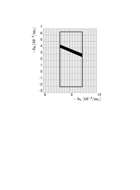
FIG. 1.: Constrains on the isoscalar and isovector scattering lengths imposed by pionic deuterium data. The black strip corresponds the one standard deviation region. The rectangle corresponds to the values obtained from pionic hydrogen data in [7].

FIG. 2.: $\sin\delta$ vs energy close to the resonance calculated from (39) for $\beta=3\,fm^{-1}$.

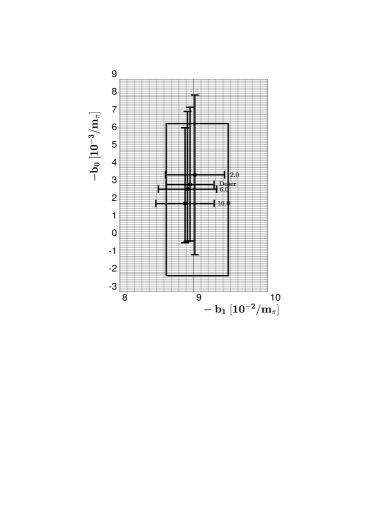
FIG. 3.: The values of isoscalar and isovector scattering lengths obtained by solving the bound state equation (32) for $\beta$ equal, respectvely, 2.0 fm^-1, 6.0 fm^-1, and 10.0 fm^-1 (indicated on the plot). The point marked as Deser has been obtained from (47). The rectangle corresponds to the values obtained in [7].

FIG. 4.: $\pi$d scattering length vs. the inverse range parameter $\beta$ of the $\pi$N potential. Full (open) circles correspond to a Faddeev calculation with (without) p-wave $\pi$N interaction.

REFERENCES

• [1] M. L. Goldberger, H. Miyazawa and R. Oehme, Phys. Rev. 99, 986 (1955).
• [2] R. A. Arndt, M. M. Pavan, R. L. Workman, and I. I. Strakovsky, Scattering Interactive Dial-Up (SAID), VPI, Blacksburg, The VPI/GWU $\pi$N solution SM99 (1999); http://said.phys.vt.edu/analysis/pin_analysis.html.
• [3] W. R. Gibbs, Li Ai and W. B. Kaufmann, Phys. Rev. C 57, 784 (1998).
• [4] A. Gashi, E. Matsinos, G. C. Oades, G. Rasche and W. S. Woolcock, Nucl. Phys A (to be published), hep-ph/0009081.
• [5] W.R. Gibbs, Li Ai and W.B. Kaufmann, Phys. Rev. Lett. 74, 3740 (1995); $\pi$N Newsletter No 11, Vol II (1995), p 84.
• [6] E. Matsinos, Phys. Rev. C 56, 3014 (1997).
• [7] D. Sigg, A. Badertscher, P. F. A. Goudsmit, H. J. L. Leisi and G. C. Oades, Nucl. Phys. A 609, 310 (1996).
• [8] H.Β C.Β SchrΓΆder, A. Badertscher, P.F.A. Goudsmit, M. Janousch, H.J. Leisi, E. Matsinos, D. Sigg, Z.G. Zhao, D. Chatellard, J.P. Egger et al., Phys.Β Lett.Β  B 469, 25 (1999).
• [9] P. Hauser, K. Kirch, L. M. Simons, G. Borchert, D. Gotta, T. Siems, P. El-Khoury, P. Indelicato, M. Augsburger, D.Β Chatellard et al., Phys. Rev. C 58, R1869 (1998).
• [10] N. Fettes, Ulf-G. Meissner and S. Steininger, Nucl. Phys. A 640, 199 (1998);
V.E. Lyubitskij and A. Russetsky, Phys. Lett. B 494, 9 (2000).
• [11] S.Β Deser, M.L.Β Goldberger, K.Β Baumann, and W.Β Thirring, Phys.Β Rev. 96, 774 (1954); T.Β L.Β Trueman, Nucl.Β Phys.Β 26, 57 (1961).
• [12] V. V. Baru and A. E. Kudryavtsev, Phys. Atom. Nucl. 60, 1475 (1997);
T.E.O. Ericson, B. Loiseau and A.W. Thomas, hep-ph/0009312.
• [13] V. V. Peresypkin and N. M. Petrov, Nucl. Phys. A 220, 277 (1974);
N. M. Petrov and V. V. Peresypkin, J. Nucl. Phys. (USSR) 18, 791 (1973).
• [14] I. R. Afnan and A. W. Thomas, Phys. Rev. C 10, 109 (1974).
• [15] T. Mizutani and D. Koltun, Ann. Phys. (NY) 109, 1 (1977).
• [16] J.M. Eisenberg and D.S. Koltun, Theory of Meson Interactions with Nuclei, (Wiley, New York 1980).
• [17] A. W. Thomas and R. H. Landau, Phys. Rep. 58, 121 (1980).
• [18] T. E. O. Ericson and W. Weise, Pions and Nuclei, (Clarendon, Oxford, 1988).
• [19] K. A. Brueckner, Phys. Rev. 89, 834 (1953).
• [20] Kerson Huang, Statistical Mechanics, (Wiley, New York 1963), Chap. XIII.
• [21] V. M. Kolybasov and A. E. Kudryavtsev, Sov. Phys. JETP 36, 18 (1973).
• [22] H. Zankel, W. Plessas and J. Haidenbauer, Phys. Rev. C 28, 538 (1983).
• [23] M. Lacombe, B. Loiseau, R. Vinh Mau, J. CΓ΄tΓ©, P. PirΓ©s, and R. de Tourreil, Phys. Lett. B 101, 139 (1981).
• [24] G. FΓ€ldt, Physica Scripta 16, 81 (1977).
• [25] R. Machleidt, K. Holinde and Ch. Elster, Phys. Rep. 149, 1 (1987), tables 11 and 13.
• [26] Handbook of Mathematical Functions, edited by M. Abramowitz and I.A. Stegun (Dover, New York, 1965).
• [27] P.B. Siegel and W. R. Gibbs, Phys. Rev. C 33, 1407 (1986).
• [28] J. Spuller, et al., Pys. Lett. B 67, 479 (1977).
• [29] W. R. Frazer and A. W. Hendry, Phys. Rev. 134 B, 1307 (1964).
• [30] W.Β B.Β Jones and W.Β J.Β Thorn, Continued fractions: Analytic Theory and Applications, (Addison-Wesley, Reading, Mass. 1980).
• [31] H. van Haeringen, Nucl. Phys. A 253, 355, (1975).
• [32] L.L. Foldy and J.D. Walecka, Ann. Phys. (N.Y.) 54, 447 (1969);
J.H. Koch and J.D. Walecka, Nucl. Phys. B 72, 283 (1974);
F.A. Gareev, M.Ch. Gizzatzulov and J. Revai, Nucl. Phys. A 286, 512 (1977).