NUC-MINN-01/8-T
Second Order Dissipative Fluid Dynamics for Ultra-Relativistic Nuclear Collisions

Abstract

The Müller-Israel-Stewart second order theory of relativistic imperfect fluids based on Grad’s moment method is used to study the expansion of hot matter produced in ultra-relativistic heavy ion collisions. The temperature evolution is investigated in the framework of the Bjorken boost-invariant scaling limit. The results of these second-order theories are compared to those of first-order theories due to Eckart and to Landau and Lifshitz and those of zeroth order (perfect fluid) due to Euler.

High energy heavy-ion collisions offer the opportunity to study the properties of hot and dense matter. To do so we must follow its space-time evolution, which is affected not only by the equation of state but also by dissipative, non-equilibrium processes. Thus we need to know the transport coefficients such as viscosity, thermal conductivity, and diffusion. We also need to know the relaxation coefficients. Knowledge of the various time and length scales is of central importance to help decide whether to apply fluid dynamics or cascade or a combination of the two. The use of fluid dynamics as one of the approaches in modeling the dynamic evolution of nuclear collisions has been successful in describing many of the observables [2, 3]. So far most work has focused on the ideal or perfect fluid and/or multi-fluid dynamics. In this work we apply the relativistic dissipative fluid dynamical approach. It is known even from non-relativistic studies [4] that dissipation might affect the observables. The first theories of relativistic dissipative fluid dynamics are due to Eckart [5] and to Landau and Lifshitz [6]. These theories are now known to have some undesirable features: they lead to Navier-Stokes-Fourier laws which are parabolic in structure and therefore may propagate signals with speeds exceeding that of light. A qualitative study of relativistic dissipative fluids for applications to relativistic heavy ions collisions has been done using these first-order theories [7].

Second-order theories of dissipative fluids due to Grad[12], Müller[13], and Israel and Stewart [14] were introduced to remedy some of these undesirable features. In second-order theories the space of thermodynamic quantities is expanded to include the dissipative quantities for the particular system under consideration. These dissipative quantities are treated as thermodynamic variables in their own right. The phenomenological formulation of the transport equations for the first-order and second-order theories is accomplished by combining the conservation of energy-momentum and particle number with the Gibbs equation. One then obtains an expression for the entropy 4-current, and its divergence leads to entropy production. Because of the enlargement of the space of variables the expressions for the energy-momentum tensor $T^{\mu\nu}$, particle 4-current $N^{\mu}$, entropy 4-current $S^{\mu}$, and the Gibbs equation contain extra terms. Transport equations for dissipative fluxes are obtained by imposing the second law of thermodynamics, that is, the principle of nondecreasing entropy. The difference between the two stems from the entropy 4-current: the standard irreversible thermodynamics of Eckart-Landau assumes that the entropy 4-current should include terms linear in dissipative fluxes and hence they are referred to as first-order theories of dissipative fluids. On the other hand the extended irreversible thermodynamics of Müller-Israel-Stewart includes terms quadratic in dissipative fluxes and hence they are referred to as second-order theories of dissipative fluids. The kinetic approach is based on Grad’s 14-moment method [12]. The resulting equations are hyperbolic and lead to causal propagations [14, 18]. For a review on generalization of the Müller-Israel-Stewart theory to a mixture of several particle species see [19].

The formulation of relativistic hydrodynamics can be found in standard text books [6, 8, 9, 10, 11]. The energy equation governing fluid motion is given by

$$D\varepsilon = -(\varepsilon+p+\Pi)\theta+\pi^{\mu\nu}\bigtriangledown_{\nu}u_{\mu}-\bigtriangledown_{\mu}q^{\mu}+q^{u}a_{\mu}\enspace,$$ (1)

where

$$\varepsilon\, \,\;\;\mbox{(energy density)}\enspace,$$ (2)

$$p\, \,\;\;\mbox{(pressure)}\enspace,$$ (3)

$$D \equiv u^{\mu}\partial_{\mu}\,\,\ \,\,\,(\mbox{convective time derivative})\enspace,$$ (4)

$$\bigtriangledown^{\mu} \equiv \bigtriangleup^{\mu\nu}\partial_{\nu}\,\,\,\,(\mbox{ gradient operator})\enspace$$ (5)

$$\theta \equiv \partial_{\alpha}u^{\alpha}\;\;\mbox{(volume expansion )}\enspace,$$ (6)

$$u^{\mu}\, \,\mbox{(4-velocity)}\enspace,$$ (7)

$$a^{\mu}\ \equiv Du^{\mu}\,\mbox{(4-acceleration)}\enspace,$$ (8)

$$\Pi\, \,\;\;\mbox{(viscous pressure)}\enspace,$$ (9)

$$\pi^{\mu\nu}\, \,\;\;\mbox{(viscous stress tensor)}\enspace,$$ (10)

$$q^{\mu}\, \,\;\;\mbox{(heat flow)}\enspace,$$ (11)

$\bigtriangleup^{\mu\nu}\equiv g^{\mu\nu}-u^{\mu}u^{\nu}$ is the projection tensor orthogonal to the 4-velocity and $g^{\mu\nu}$ = diag$(+1,-1,-1,-1)$ is the metric tensor in Minkowski space-time. In the Eckart theory the dissipative contribution to the bulk pressure, the heat flux and the shear viscous tensor are given by

$$\Pi = -\zeta\theta\enspace,$$ (12)

$$q^{\mu} = \lambda T\left(\frac{\bigtriangledown^{\mu}T}{T}-a^{\mu}\right)\enspace,$$ (13)

$$\pi^{\mu\nu} = 2\eta\bigtriangledown^{\langle\mu}u^{\nu\rangle}\enspace,$$ (14)

where $\zeta\,,\eta\,,\lambda$ are the bulk, shear and thermal conductivity coefficients respectively. They are required to be positive by the second law of thermodynamics. $T$ is the temperature of the system. The angular bracket notation is defined by:

$$A^{<\mu\nu>} \equiv \left[\frac{1}{2}\left(\bigtriangleup^{\mu}_{\sigma}\bigtriangleup^{\nu}_{\tau}+\bigtriangleup^{\mu}_{\tau}\bigtriangleup^{\nu}_{\sigma}\right)-\frac{1}{3}\bigtriangleup^{\mu\nu}\bigtriangleup_{\sigma\tau}\right]A^{\sigma\tau}\enspace.$$ (15)

The above expressions for dissipative fluxes can also be obtained in kinetic theory by employing the first Chapman-Enskog approximation [15]. In second-order theories we have to solve for these dissipative fluxes from their evolution equations. One can show [16] that in the 1+1 Bjorken scaling solution hypothesis [17], the system of transport equations given by [14] becomes tractable. The same simplifications occur in 1+1 dimensional Bjorken hypothesis in first order dissipative fluid calculations [7]. In 2+1 and 3+1 dimensional flow these equations become much more complicated. This is a subject of current study [16].

I give here the second-order equations for 1+1 dimensional scaling solution. These equations were derived from kinetic theory using Grad’s 14-moment approximation method [12]. We will only need the Müller-Israel-Stewart [14] equations in the following form:

$$D\Pi = -\frac{1}{\tau_{\Pi}}\Pi-\frac{1}{2}\frac{1}{\beta_{0}}\Pi\left(\beta_{0}\theta+TD\left(\frac{\beta_{0}}{T}\right)\right)$$ (17)

$$-\frac{1}{\beta_{0}}\theta\enspace,$$

$$Dq^{\mu} = -\frac{1}{\tau_{q}}q^{\mu}+\frac{1}{2}\frac{1}{\beta_{1}}q^{\mu}\left(\beta_{1}\theta+TD\left(\frac{\beta_{1}}{T}\right)\right)$$ (19)

$$+\frac{1}{\beta_{1}}\left(\frac{\bigtriangledown^{\mu}T}{T}-a^{\mu}\right)\enspace,$$

$$D\pi^{\mu\nu} = -\frac{1}{\tau_{\pi}}\pi^{\mu\nu}-\frac{1}{2}\frac{1}{\beta_{2}}\pi^{\mu\nu}\left(\beta_{2}\theta+TD\left(\frac{\beta_{2}}{T}\right)\right)$$ (21)

$$+\frac{1}{\beta_{2}}\bigtriangledown^{\langle\mu}u^{\nu\rangle}\enspace,$$

where

$$\tau_{\Pi}=\zeta\beta_{0}\,\,\,\,,\tau_{q}=\lambda T\beta_{1}\,\,\,\,,\tau_{\pi}=2\eta\beta_{2}\enspace,$$ (22)

are the relaxation times, $\beta_{0}\,,\beta_{1}$ and $\beta_{2}$ are the relaxation coefficients. These three new coefficients are functions of primary thermodynamic variables like pressure, number density and energy density and hence depend on the equation of state. Relaxation time is the distinguishing feature of hyperbolic causal theories which is not present in the first-order theories. Here $\tau_{i}$ is the time taken by the corresponding dissipative flux to relax to its steady-state value.

For the 1+1 dimensional Bjorken [17] similarity fluid flow the energy equation becomes:

$$\frac{d\varepsilon}{d\tau}+\frac{\varepsilon+p}{\tau}-\frac{2}{3}\frac{1}{\tau}\Phi+\Pi\frac{1}{\tau}=0\enspace,$$ (23)

where $\Phi\equiv\pi^{00}-\pi^{zz}$ is determined from the shear viscous tensor evolution equation

$$\frac{d}{d\tau}\Phi = -\frac{1}{\tau_{\pi}}\Phi-\frac{1}{2}\Phi\left(\frac{1}{\tau}+\frac{1}{\beta_{2}}T\frac{d}{d\tau}\left(\frac{\beta_{2}}{T}\right)\right)+\frac{2}{3}\frac{1}{\beta_{2}}\frac{1}{\tau}\enspace.$$ (24)

The equation for $\Pi$ will not needed as explained below. For this initial study a simple equation of state is used, namely that of a weakly interacting plasma of massless $u\,,d\,,s\,$ quarks and gluons. The pressure is given by $p=\varepsilon/3=aT^{4}$ with zero baryon chemical potential. Here $a$ is a constant determined by the number of quark flavors and the number of gluon colors. In the case of massless particles the bulk pressure equation (17) does not contribute since the bulk viscosity is negligible or vanishes [8]. The only relaxation coefficient we need is $\beta_{2}$ which for massless particles is given by $\beta_{2}=3/(4p)$. The shear viscosity is given by [20] $\eta=bT^{3}$ where $b$ is a constant determined by the number of quark flavors and the number of gluon colors. The energy equation (1) and the viscous stress tensor equation (21) can be written as

$$\frac{d}{d\tau}T = -\frac{T}{3\,\tau}+\frac{T^{-3}\Phi}{18\,a\,\tau}\enspace,$$ (25)

$$\frac{d}{d\tau}\Phi = -\frac{2\,a\,T\Phi}{3\,b}-\frac{1}{2}\left(\frac{1}{\tau}-5\frac{1}{T}\frac{d}{d\tau}T\right)\Phi+\frac{8\,a\,T^{4}}{9\,\tau}\enspace.$$ (26)

where

$$a = \left(16+\frac{21}{2}N_{f}\right)\frac{\pi^{2}}{90}\enspace,$$ (27)

$$b = \left(1+1.70N_{f}\right)\frac{0.342}{(1+N_{f}/6)\,\alpha_{s}^{2}\ln(\alpha_{s}^{-1})}\enspace,$$ (28)

Here $N_{f}$ is the number of quark flavors, taken to be $3$, and $\alpha_{s}$ is the strong fine structure constant taken to be $0.5$. For a perfect fluid and a first-order theory the energy equation (23) can be solved analytically to give

$$T(\tau) = T_{0}\left[\frac{\tau_{0}}{\tau}\right]^{1/3}~{}~{}~{}~{}~{}\mbox{(perfect fluid)}\enspace,$$ (29)

$$T(\tau) = T_{0}\left[\frac{\tau_{0}}{\tau}\right]^{1/3}\left\{1+\frac{b}{6\,a}\frac{1}{T_{0}\,\tau_{0}}\left(1-\left[\frac{\tau_{0}}{\tau}\right]^{2/3}\right)\right\}$$ (31)

$$\mbox{(first-order theory)}\enspace,$$

In the first order theory we do not have the relaxation coefficients. Then equation (24) gives $\Phi=(4\eta/3)/\tau$. The above equations and the numerical solution to the second-order equations (25) and (26) are presented in Figs. 1 through 4. We choose the initial temperatures to correspond to those expected at RHIC and LHC, namely $T_{0}$=500 MeV at RHIC and $T_{0}$=1000 MeV at LHC. In Figs. 1 and 2 the initial time $\tau_{0}$ is estimated by using the uncertainty principle [21]: $\tau_{0}\cdot{\langle E\rangle}_{0}\sim 1$ where ${\langle E\rangle}_{0}\sim 3T_{0}$ for massless particles. This results in $\tau_{0}$=0.13 fm/c at RHIC and $\tau_{0}$=0.07 fm/c at LHC. The initial value used for $\Phi$, which must be specified independently for the second order theory, is taken to be $p/3$. We choose this value since the second order theory is based on the assumption that the dissipative fluxes are small compared to the primary thermodynamic variables, namely $p,n,$and $\varepsilon$. However, a thorough study of the initial conditions on these dissipative fluxes is needed and should perhaps be found from microscopic models. This is as subject of current study [16]. The effect of dissipation is more pronounced at the very early stages of heavy ion collisions when gradients of temperature, velocity, etc., are large. At late times the effect of dissipation vanishes. In Figs. 3 and 4 we take a constant initial time $\tau_{0}$=1.0 fm/c which is the characteristic hadronic time scale. Euler hydrodynamics predicts the fastest cooling. The first-order theory significantly under-predicts the work done during the expansion relative to the Müller-Israel-Stewart and Euler predictions. Thus the temperature decreases more slowly with the inclusion of dissipative effects. This would lead to greater yields of photons and dileptons, and also the transverse energy/momentum would be reduced as the collective velocities are dissipated into heat. The system takes longer to cool down. This will delay freeze-out. Also entropy, $s=4\,a\,T^{3}$, is enhanced. This is important because entropy production can be related to final multiplicity. With respect to entropy production due to particle production, see [22]. Given some initial conditions we want to investigate the importance of second order theories as compared to first order theories and perfect fluids. Let us now analyze the differences between the second-order and first-order theories. The first thing we notice is that the Eckart-Landau theory predicts that at early times the temperature will first rise before falling off. This is more pronounced when we have small initial times. Naively one would expect that the system would cool monotonically as it expands even in the case of dissipation where energy-momentum is conserved. On the other hand, it is seen that for large initial times and high temperatures the three theories have a similar time evolution. As can be seen from Fig. 4, all three cases start at the same point and then fall off with time. The difference stems from the fact that in the second-order theory the transport equations of the dissipative fluxes describe the evolution of these fluxes from an arbitrary initial state to an equilibrium state. The first-order theory, though, is just related to the thermodynamic forces which, if switched off, do not demonstrate relaxation. Hence they are sometimes referred to as quasi-stationary theories. As can be seen from Fig. 4, it is before the establishment of an equilibrium state that the two theories differ significantly. In ultra-relativistic heavy ion collisions, where the fluid evolution occurs in very short times, the second-order theories should be used to analyze collision dynamics. In doing so a full analysis requires that all the dynamical equations with more realistic equations of state and transport coefficients be considered

I will conclude by pointing out some of the advantages and challenges of the second-order theories. Second-order theories, being hyperbolic in structure, lead to well-posed initial-value (Cauchy) problems. They also lead to causal propagation. Unlike the first-order theories, second-order theories have relaxation terms which permit us to study the evolution of the dissipative fluxes. The challenge we face is the increase in the space of thermodynamic variables. We now have, in addition to the transport coefficients, new coefficients in the problem. These are the relaxation coefficients $\beta_{i}$ and the coupling coefficients $\alpha_{i}$. These new coefficients depend on the primary thermodynamic variables, such as $n,\varepsilon$ and $p$ and therefore are determined by the equation of state. Like viscosity and thermal conductivity, which are required to be positive by the second law of thermodynamics, these new coefficients are constrained by hyperbolicity requirements. In principle , in order to solve the second-order relativistic dissipative fluid dynamic problem, one still needs the equation of state, initial conditions and the transport coefficients.

To probe non-equilibrium properties of matter produced in heavy ion collisions we need a non-equilibrium fluid dynamics model to analyze observables. The relativistic fluid dynamics modeling of heavy ion collisions will have to include dissipation and thermal conduction. One will then have to use the hyperbolic theories of relativistic dissipative fluids because of their universality. Hyperbolic theories might prove to be convenient in constructing hydro-molecular dynamic schemes [23] in which a phenomenological fluid dynamics model is coupled to a microscopic kinetic model such that microscopic kinematic quantities may be obtained. Dissipation mechanism might be important if we deal with the event-by-event based hydrodynamics [24].

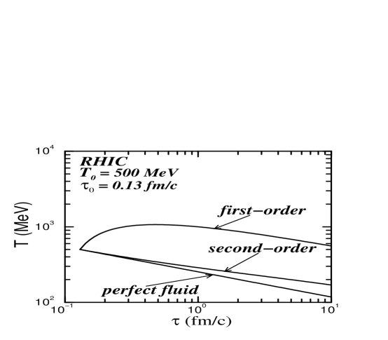
FIG. 1.: Proper time evolution of temperature for a RHIC scenario: $\tau_{0}$ = 0.13 fm/c and $T_{0}$ = 500 MeV .

FIG. 2.: Proper time evolution of temperature for a LHC scenario: $\tau_{0}$ = 0.07 fm/c and $T_{0}$ = 1000 MeV .

FIG. 3.: Proper time evolution of temperature for a RHIC scenario: $\tau_{0}$ = 1.0 fm/c and $T_{0}$ = 500 MeV.

FIG. 4.: Proper time evolution of temperature for a LHC scenario: $\tau_{0}$ = 1.0 fm/c and $T_{0}$ = 1000 MeV.

- [1] Electronic address: amuronga@physics.spa.umn.edu
- [2] H. Stöcker and W. Greiner, Phys. Rep. 137, 227 (1986); R. B. Clare and D. Strottman, Phys. Rep. 141, 177 (1986).
- [3] K. Kajantie, M. Kataja, L. McLerran and P.V. Russskanen, Phys. Rev. D 34, 2746 (1986); E.F. Staubo, A.K. Holme, L.P. Csernai, M. Gong and D. Strottman, Phys. Lett. B229, 351 (1989); I.N. Mishustin, V.N. Russkikh and L.M. Satarov, Nucl. Phys. A494, 595(1989); U. Katscher, D.H. Rischke, J.A. Maruhn, W. Greiner, I.N Mishustin and L.M. Satarov, Z. Phys. A346, 209 (1993).
- [4] J.I. Kapusta, Phys. Rev. C 24, 2545 (1981).
- [5] C. Eckart, Phys. Rev. 58, 919 (1940).
- [6] L. D. Landau and E. M. Lifshitz, Fluid Mechanics, (Addison-Wesley, Reading, Massachusetts, 1959).
- [7] K. Kajantie, Nucl. Phys. A418, 41c (1984); G. Baym, Nucl. Phys. A418 525c (1984); A. Hosoya and K. Kajantie, Nucl. Phys. B250, 666 (1985); P. Danielewicz and M. Gyulassy, Phys. Rev. D 31, 53 (1985); L. Mornas and U. Ornik, Nucl. Phys. A587, 828 (1995); H. Kouno, M. Maruyama, F. Takagi and K. Saigo, Phys. Rev. D 41, 2903 (1990); R. Hakim and L. Mornas, Phys. Rev. C 47, 2846 (1993).
- [8] S. Weinberg, Gravitation and Cosmology: Principles and Applications of the General Theory of Relativity (J. Willey and Sons, New York, 1972).
- [9] L.P. Csernai, Introduction to Relativistic Heavy Ion Collisions (J. Wiley and Sons, New York, 1994).
- [10] S.R. de Groot, H.A. van Leeuven and C.G. van Weert, Relativistic Kinetic Theory (North-Holland, Amsterdam, 1980).
- [11] D.H. Rischke, in Hadrons in Dense Matter and Hadrosynthesis, J. Cleymans, H.B. Geyer and F.G. Scholtz (Eds.), (Lecture Notes in Physics, Vol. 516, Springer, 1999).
- [12] H. Grad, Commun. Pure Appl. Math. 2, 331 (1949).
- [13] I. Müller, Z. Phys. 198, 329 (1967).
- [14] W. Israel, Ann. Phys. (N.Y.) 100, 310 (1976); J.M. Stewart, Proc. Roy. Soc. A357, 59 (1977); W. Israel and J.M. Stewart, Ann. Phys. (N.Y.) 118,( 341 (1979).
- [15] S. Chapman and T.G. Cowling, The Mathematical Theory of Non-Uniform Gases, Third Edition (Cambridge University Press, Cambridge, 1970).
- [16] Detailed calculations to be published in PhD thesis.
- [17] J.D. Bjorken, Phys. Rev. D 27, 140 (1983).
- [18] W.A. Hiscock and L. Lindblom, Ann. Phys. (N.Y.) 151, 466 (1983); Phys. Rev. D 31, 725 (1985); ibid. 35, 3723 (1987).
- [19] M. Prakash, M. Prakash, R. Venugopalan and G. Welke, Phys. Rep. 227, 321 (1993).
- [20] G. Baym, H. Monien, C.J. Pethick and D.G. Ravenhall, Phys. Rev. Lett. 64, 1867 (1990).
- [21] J. Kapusta, L. McLerran and D. K. Srivastava, Phys. Lett. B283, 145 (1992).
- [22] H.-Th. Elze, J. Rafelski and L. Turko, Phys. Lett. B506, 123 (2001).
- [23] S.A. Bass, and A. Dumitru, Phys. Rev. C 61, 064909, 2000.
- [24] C.E. Aguiar, T. Kodama, T. Osada and Y. Hama, J. Phys. G27, 75 (2001).