Nucleon-Nucleon Scattering in a Three-Dimensional Approach

Two-nucleon scattering at intermediate energies of a few hundred MeV requires quite a few angular momentum states in order to achieve convergence of e.g. scattering observables. This is even more true for the scattering of three or more nucleons upon each other. An alternative approach to the conventional one, which is based on angular momentum decomposition, is to work directly with momentum vectors, specifically with the magnitudes of momenta and the angles between them. We formulate and numerically illustrate [1] this alternative approach for the case of NN scattering using two realistic interaction models, the Argonne AV18 [2] and the Bonn-B [3] potentials. The momentum vectors enter directly into the scattering equation, and the total spin of the two nucleons is treated in a helicity representation with respect to the relative momenta $\bf q$ of the two nucleons.

The momentum-helicity states are given as

$$\left|{\bf q};\hat{q}S\Lambda\right\rangle\equiv\left|{\bf q}\right\rangle\left|\hat{q}S\Lambda\right\rangle=\left|{\bf q}\right\rangle R(\hat{q})\sum_{m_{1}m_{2}}C(\frac{1}{2}\frac{1}{2}S;m_{1}m_{2}\Lambda)\left|\hat{z}\frac{1}{2}m_{1}\right\rangle\left|\hat{z}\frac{1}{2}m_{2}\right\rangle,$$ (1)

where $R(\hat{q})=\exp(-iS_{z}\phi)\exp(-iS_{y}\theta)$ is the rotation operator, $S_{z},\,S_{y}$ the components of ${\bf S}=\frac{1}{2}({\mbox{\boldmath$\sigma$}}_{1}+{\mbox{\boldmath$\sigma$}}_{2})$, and $\Lambda$ the eigenvalue of the helicity operator ${\bf S}\cdot\hat{q}$. Introducing parity and two-body isospin states $|tm_{t}\rangle$, the antisymmetrized two-nucleon state is given by

$$\left|{\bf q};\hat{q}S\Lambda;t\right\rangle^{\pi a}=\frac{1}{\sqrt{2}}(1-\eta_{\pi}(-)^{S+t})\left|t\right\rangle\left|{\bf q};\hat{q}S\Lambda\right\rangle_{\pi},$$ (2)

with the parity eigenvalues $\eta_{\pi}=\pm 1$ and $\left|{\bf q};\hat{q}S\Lambda\right\rangle_{\pi}\equiv\frac{1}{\sqrt{2}}(\left|{\bf q}\right\rangle+\eta_{\pi}\left|-{\bf q}\right\rangle)\left|\hat{q}S\Lambda\right\rangle$.

With these basis states we formulate the Lippmann-Schwinger (LS) equations for NN scattering. In the singlet case, $S=0$, there is one single equation for each parity,

$$T_{00}^{\pi St}({\bf q}^{\prime},{\bf q})=V_{00}^{\pi St}({\bf q}^{\prime},{\bf q})+\frac{1}{4}\int d^{3}q^{\prime\prime}\,V_{00}^{\pi St}({\bf q}^{\prime},{\bf q}^{\prime\prime})G_{0}(q^{\prime\prime})T_{00}^{\pi St}({\bf q}^{\prime\prime},{\bf q})$$ (3)

Using rotational and parity invariance one finds in the triplet case, $S=1$, a set of two coupled LS equations for each parity and each initial helicity state

$$T_{\Lambda^{\prime}\Lambda}^{\pi St}({\bf q}^{\prime},{\bf q}) = V_{\Lambda^{\prime}\Lambda}^{\pi St}({\bf q}^{\prime},{\bf q})+\frac{1}{2}\int d^{3}q^{\prime\prime}\,V_{\Lambda^{\prime}1}^{\pi St}({\bf q}^{\prime},{\bf q}^{\prime\prime})G_{0}(q^{\prime\prime})T_{1\Lambda}^{\pi St}({\bf q}^{\prime\prime},{\bf q})$$ (4)

$$+\frac{1}{4}\int d^{3}q^{\prime\prime}\,V_{\Lambda^{\prime}0}^{\pi St}({\bf q}^{\prime},{\bf q}^{\prime\prime})G_{0}(q^{\prime\prime})T_{0\Lambda}^{\pi St}({\bf q}^{\prime\prime},{\bf q}).$$

Because of the symmetry properties only two $(\Lambda=1,0)$ of the original three initial helicity states need to be considered. Both LS equations are two-dimensional integral equations in two variables for the half-shell t-matrix and in three variables for the fully-off-shell t-matrix, namely two magnitudes of momenta and one angle. For explicit calculations we choose $\hat{q}=\hat{z}$, which allows together with the properties of the potential that the azimuthal dependence of $\bf q^{\prime}$ and $\bf q$ can be factored out

$$T_{\Lambda^{\prime}\Lambda}^{\pi St}({\bf q}^{\prime},{\bf q})=e^{i\Lambda(\phi^{\prime}-\phi)}T_{\Lambda^{\prime}\Lambda}^{\pi St}(q^{\prime},q,\theta^{\prime}).$$ (5)

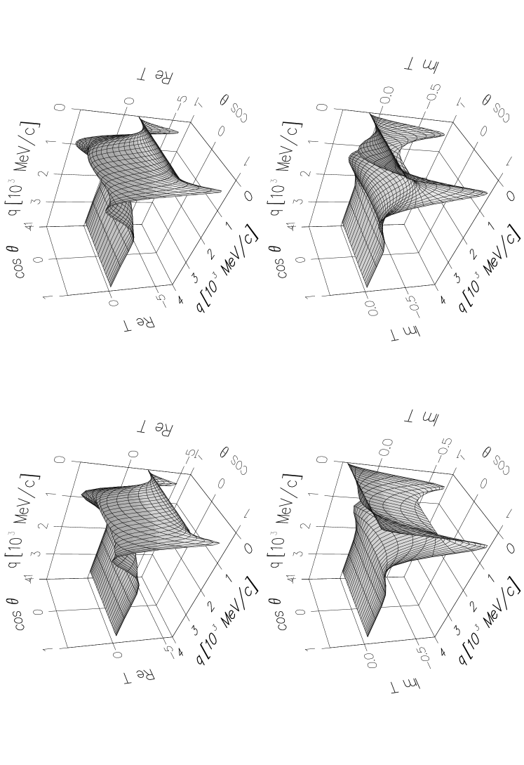
Figure 1: $T^{101}_{00}(q,q_{0},\theta)$ as a function of $q$ and $\cos\theta$ in units of $10^{-7}$ MeV^-2. Left side for Bonn-B, right side for AV18.

As it is well known, rotational-, parity-, and time reversal invariance restricts any NN potential V to be formed out of six independent terms [4]. We introduce the following set of linear independent operators, which are diagonal in our basis

$$\Omega_{1}=1\> \>\Omega_{2}={\bf S}^{2}$$ ;

$$\Omega_{3}={\bf S}\cdot\hat{q}^{\prime}\,{\bf S}\cdot\hat{q}^{\prime}\> \>\Omega_{4}={\bf S}\cdot\hat{q}^{\prime}\,{\bf S}\cdot\hat{q}$$ ;

$$\Omega_{5}=({\bf S}\cdot\hat{q}^{\prime})^{2}\,({\bf S}\cdot\hat{q})^{2}\> \>\Omega_{6}={\bf S}\cdot\hat{q}\,{\bf S}\cdot\hat{q}$$ ; (6)

and represent the most general potential in a nonrelativistic Schrödinger equation as linear combination of them,

$$\langle{\bf q^{\prime}}|V|{\bf q}\rangle\equiv V({\bf q^{\prime}},{\bf q})=\sum_{i=1}^{6}v_{i}(q^{\prime},q,\gamma)\Omega_{i}.$$ (7)

Here $v_{i}(q^{\prime},q,\gamma)$ are scalar functions of the magnitudes of the vectors $\bf q^{\prime}$, $\bf q$, and the angle $\gamma={\hat{q}}^{\prime}\cdot{\hat{q}}$ between them. It should be noted that for $\bf q$ pointing in $z$-direction one can use $\left\langle\hat{q}^{\prime}S\Lambda^{\prime}\right.\left|\hat{z}S\Lambda\right\rangle=\exp(i\Lambda(\phi^{\prime}-\phi))d^{S}_{\Lambda\Lambda^{\prime}}(\theta^{\prime})$, so that the azimuthal dependence factors out of V and thus also out of the T-matrix. The operators $\Omega_{i}$ can be transformed to the standard Wolfenstein form [4] with a linear transformation as shown in [1].

To demonstrate the feasibility of our formulation when applied to NN scattering we present numerical results for two different NN potentials of quite different character, the Bonn-B [3] and the AV18 [2] potential models. Similarities and differences in the half-shell T-matrices $T^{\pi St}_{\Lambda^{\prime}\Lambda}(q,q_{0},\theta)$ are displayed for $T^{101}_{00}(q,q_{0},\theta)$ for $q_{0}=375~{}MeV/c$ in Fig. 1. The amplitudes are identical on-shell and show deviations off-shell. The choice presented in Fig. 1 is quite representative for the off-shell differences between the two models.

Figure 2: $|\langle++|T|--\rangle|^{2}$ and $|\langle++|T|++\rangle|^{2}$ in units of $10^{-14}$ MeV^-4 as a function of $x=\cos\theta$ for $q_{0}$=375 MeV/c.

In order to connect with standard representations of the NN t-matrix as well as to calculate observables, we express $T$ in terms of antisymmetric states

$$\left|\tau_{1}\tau_{2}m_{1}m_{2}{\bf q}\right\rangle_{a}\equiv\frac{1}{\sqrt{2}}(1-P_{12})\left|\tau_{1}\tau_{2}m_{1}m_{2}{\bf q}\right\rangle,$$ (8)

where $\tau_{i}$ and $m_{i}$ are the magnetic isospin and spin quantum numbers and $P_{12}$ is the permutation operator of the two nucleons. In this representation, which we denote as ‘physical’, we obtain for the on-shell T-matrix elements ( $|\bf q^{\prime}|=|\bf q|$)

$${}_{a}\langle\tau_{1}\tau_{2}m_{1}^{\prime}m_{2}^{\prime}q\hat{q}^{\prime}| T |\tau_{1}\tau_{2}m_{1}m_{2}{\bf q}\rangle_{a}=\frac{1}{4}e^{-i(\Lambda_{0}^{\prime}-\Lambda_{0})\phi^{\prime}}\sum_{S\pi t}C(\frac{1}{2}\frac{1}{2}t;\tau_{1}\tau_{2})^{2}(1-\eta_{\pi}(-)^{S+t})$$ (9)

$$\quad C(\frac{1}{2}\frac{1}{2}S;m_{1}^{\prime}m_{2}^{\prime}\Lambda_{0}^{\prime})C(\frac{1}{2}\frac{1}{2}S;m_{1}m_{2}\Lambda_{0})\sum_{\Lambda^{\prime}}d^{S}_{\Lambda_{0}^{\prime}\Lambda^{\prime}}(\theta^{\prime})T_{\Lambda^{\prime}\Lambda_{0}}^{\pi St}(q,q,\theta^{\prime}).$$

The quantity $T_{\Lambda^{\prime}\Lambda_{0}}^{\pi St}(q,q,\theta^{\prime})$ can be related through straightforward but lengthy algebra to the standard partial wave T-matrix $T^{Sjt}_{l^{\prime}l}(q)$ as is shown in [1]. Here we want to consider the on-the-energy-shell amplitudes $|_{a}\langle\tau_{1}\tau_{2}m_{1}^{\prime}m_{2}^{\prime}q_{0}\hat{q}|T|\tau_{1}\tau_{2}m_{1}m_{2}{\bf q_{0}}\rangle_{a}|^{2}\equiv|\langle m_{1}^{\prime}m_{2}^{\prime}|T|m_{1}m_{2}\rangle|^{2}$, $m=\pm\frac{1}{2}$. If one takes rotational symmetry and parity invariance into account, one ends up with six independent amplitudes out of the 16 possible combinations. Two of them, $|\langle++|T|--\rangle|^{2}$ and $|\langle++|T|++\rangle|^{2}$, are displayed in Fig. 2 as a function of $\cos\theta$ where $\theta$ is c.m. angle for a projectile energy of 300 MeV ($q_{0}$=375 MeV/c). In addition to the result from the 3D calculation we show the partial wave sums for increasing $j_{max}$. One can clearly see that at $E_{lab}$=300 MeV partial waves up to at least $j_{max}$=12 are needed to obtain a converged result for every matrix element.

From the ‘physical’ T-matrix amplitudes we construct the Wolfenstein amplitudes [5]. Once those are obtained it is straightforward to calculated the NN scattering observables [6]. In order to unambiguously define the normalization we also give the expression for the spin-averaged differential cross section for nucleon species $\tau_{1}\tau_{2}$ as

$$\frac{d\sigma}{d\Omega}=(2\pi)^{4}\left(\frac{m}{2}\right)^{2}\frac{1}{4}\sum_{m^{\prime}_{1}m^{\prime}_{2}m_{1}m_{2}}|_{a}\langle\tau_{1}\tau_{2}m_{1}^{\prime}m_{2}^{\prime}q{\hat{q}}^{\prime}|T|\tau_{1}\tau_{2}m_{1}m_{2}{\bf q}\rangle_{a}|^{2}$$ (10)

In Fig. 3 the differential cross section is given for $E_{lab}$=300 MeV together with partial wave sums for increasing $j_{max}$. It should be noted that the convergence of the partial wave sums is especially slow for the backward angle differential cross section. A sum up to $j_{max}$=16 is needed to obtain convergence within 1 %. In Fig. 4 $A_{y}$ is displayed, which needs a partial wave sum up to $j_{max}$=10 to reach a similar convergence.

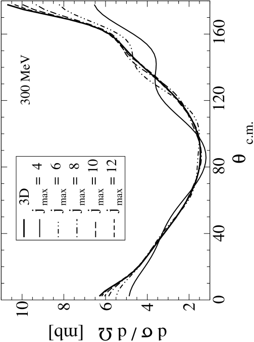
Figure 3: $\frac{d\sigma}{d\Omega}$ as a function of $\theta$ for $q_{0}$=375 MeV/c.

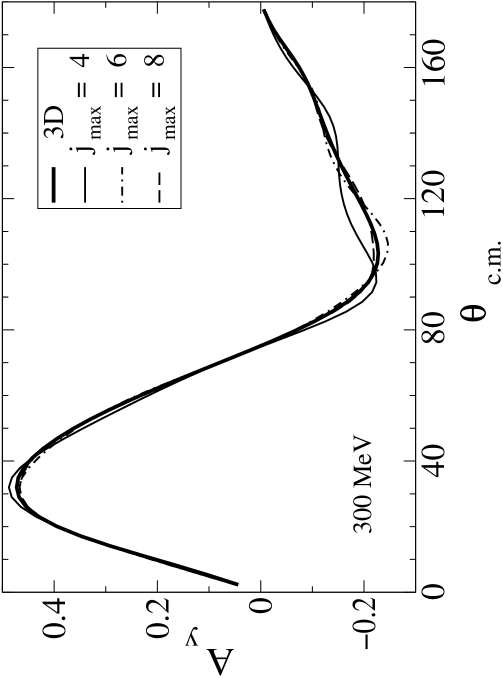
Figure 4: $A_{y}$ as a function of $\theta$ for $q_{0}$=375 MeV/c.

In summary, we formulated and numerically illustrated an alternative approach to NN scattering which works directly with momentum vectors. The spin of the two nucleons is treated in a helicity representation with respect to the relative momentum of the two nucleons. We would like to emphasize that the here developed scheme is algebraically quite simple to handle provided potentials are given in an operator form. This is e.g. the case for all interactions developed within a field theoretic frame work. This work is intended to serve as starting point towards treating three-nucleon scattering in a similar fashion.

References

[1] I. Fachruddin, Ch. Elster, W. Glöckle, http://xxx.lanl.gov/ps/nucl-th/0004057, and to be published in Phys. Rev. C.
[2] R. B. Wiringa, V. G. J. Stoks, R. Schiavilla, Phys. Rev.
C51, 38 (1995).
[3] R. Machleidt, Adv. Nucl. Phys. 19, 189 (1989).
[4] L. Wolfenstein, Phys. Rev. 96, 1654 (1954).
[5]
W. Glöckle, The Quantum-Mechanical Few-Body Problem, Springer Verlag, Berlin,
Heidelberg 1983.
[6] N. Hoshizaki, Suppl. Prog. Theor. Phys. 42, 1968.