Changes in $r$-process abundances at late times

Abstract

We explore changes in abundance patterns that occur late in the $r$ process. As the neutrons available for capture begin to disappear, a quasiequilibrium funnel shifts material into the large peaks at $A=130$ and $A=195$, and into the rare-earth “bump” at $A=160$. A bit later, after the free-neutron abundance has dropped and beta-decay has begun to compete seriously with neutron capture, the peaks can widen. The degree of widening depends largely on neutron-capture rates near closed neutron shells and relatively close to stability. We identify particular nuclei the capture rates of which should be examined experimentally, perhaps at a radioactive beam facility.

]

I Introduction

The $r$ process, which synthesizes roughly half the elements with atomic number $A>70$, proceeds through neutron capture and beta decay [1, 2, 3]. Through most of the process, we know, capture is much faster than beta decay, so that very neutron-rich and unstable nuclei are temporarily created before disappearing as the process peters out. The question of where the nucleosynthesis occurs, however, is still unanswered. An evacuated bubble expanding behind a supernova shock waves is a promising candidate for the site, but not yet the clear choice. The scenario is more convincing if the initial expansion is very rapid [4], but simple models of fast adiabatic expansion [5] imply that the neutron capture must finish in less than a second. In traditional simulations, where capture must often wait for a nucleus to beta decay, the process takes 2 or 3 times that long.

Simulations from, e.g., ref. [5] demonstrate that the entire process can take place quickly if neutron capture populates nuclei farther from stability (and thus shorter lived) than usually thought. Despite initially forming at lower $Z$ and $A$ than traditional work suggests, the simulated abundance peaks end up at the right atomic numbers. The apparent reason is that nuclei in the peak move up quickly in $Z$ through an alternating sequence of beta-decay and neutron capture near the end of the $r$ process, when the supply of free neutron begins to run out but before neutron capture completely stops. But how do peaks maintain themselves during this late time, as beta decay drives each nucleus at a different rate towards stability? This question is actually more general than the rapid-expansion scenario; a quick move towards stability while the neutron abundance drops, though most dramatic if the path is initially very far away, in fact characterizes all bubble $r$-process simulations that produce something like the correct abundance distribution. And the question is linked to a broader issue: the significance of neutron capture once the process has slowed down so that it must compete with beta decay. What happens if the capture rates then are faster or slower than we think? In which nuclei do capture rates have the largest effects on final abundances, and can the rates there be measured? These are the kinds of issues we address here.

The late stages of neutron capture and beta decay in the $r$ process are much different from what precedes them. When the neutron-to-nucleus ratio $R$ is much larger than 1, equilibrium between neutron capture and photodisintegration is a good approximation; the “path” consisting of the most abundant isotopes for each element $Z$ is far from stability and moves relatively slowly. The term “steady state” is sometimes used to refer to this period, which ends when the neutron-to-seed ratio $R$ falls below a few. To see what happens next, we note that the neutron separation energies along the path in $(n,\gamma)\leftrightarrow(\gamma,n)$ equilibrium are related to the neutron number density $n_{n}$, which is proportional to $R$ for slowly changing matter densities, by

$$S_{n}\approx-kT\ln\left\{{n_{n}\over 2}\left({2\pi\hbar^{2}\over m_{n}kT}\right)^{3/2}\right\}~{},$$ (1)

where $m_{n}$ is the neutron mass. When $R$ drops below about 1, a nucleus on the path that beta-decays can no longer capture enough free neutrons to return to the path so that the path itself must move instead, inwards to higher neutron separation energy. The increased average neutron binding makes photodisintegration less effective, which in turn reduces the number of free neutrons still further, in accordance with eq. 1. The process feeds on itself, causing $R$ to drop exponentially and the $r$-process path to move quickly towards stability. Soon $R$ becomes so small that $(n,\gamma)\leftrightarrow(\gamma,n)$ equilibrium begins to fail, and beta decay moves a good fraction of nuclei away from the path. Eventually, beta decay becomes faster than neutron capture and all remnants of $(n,\gamma)\leftrightarrow(\gamma,n)$ equilibrium vanish. The inability of equilibrium to maintain itself on the time scale of beta decay is usually called “freezeout”.

To answer the questions about peak evolution and the significance of neutron capture at late times, we focus on two competing effects. The first, which dominates just as $R$ falls below a few, when $(n,\gamma)\leftrightarrow(\gamma,n)$ equilibrium still holds well, is a funneling of material into moving peaks, most notably the small rare-earth peak [6], but also the larger peaks at $A=130$ and 195. As time passes, the funnel fights an increasing tendency for the peaks to spread because beta decay and beta-delayed neutron emission compete harder with neutron capture. The interplay of funneling and spreading will imply that uncertain neutron capture rates, which are irrelevant as long as $(n,\gamma)\leftrightarrow(\gamma,n)$ equilibrium holds, become important fairly near stability, and should be determined there more precisely.

We support our contentions with simulations of the neutron-capture part of the $r$ process. In most, we explore late times without worrying about a fast $r$ process. We assume an exponential decay of temperature and density with a relatively slow time scale of 2.8 seconds, the same as in ref. [7]. The distribution of seed nuclei with which we start is the post-alpha-process distribution of ref. [7], and we vary the initial temperature (and thus the initial density, since we keep the entropy equal to 300) and neutron-to-seed ratio. What we call our “standard simulation” is run under these conditions with the intial temperature fixed at $T_{9}=1.5$. In section III, we worry more about a fast $r$ process and therefore use different conditions. We do this in two ways: the first is to use use the same temperature and density dependence as described above, but a greater initial density (and thus a lower entropy). The faster neutron capture at high density pushes the path farther from stability and leads to the formation of the $A=195$ peak and the exhaustion of free neutrons in only tenths of a second. The second way is to use the conditions of Ref. [5], where the temperature and density drop with a time scale of 50 ms and then level off at low values ($T_{9}<1$, $\rho<100~{}{\rm g/cm^{3}}$). The resulting drop in photodissociation rates again moves the path farther from stability, and the $A=195$ peak forms in under a second. All our simulations use nuclear masses from ref. [8] and beta-decay rates from ref. [9].

The rest of this paper is organized as follows: In Section II, we discuss the action of funneling and spreading in the formation of the rare-earth element bump. Section III applies the same ideas to the large peaks, with emphasis on the change in the peak’s location and width as the path moves. The most important results appear in Section IV, which discusses neutron capture near the peaks and isolates particularly important rates that should be measured. Section V is a conclusion.

II Funneling and spreading in the rare earth region

Ref. [6] presented the basic dynamics of the near-freezeout funnel. It concluded that for much of the time when $R<1$, the system is still nearly in $(n,\gamma)\leftrightarrow(\gamma,n)$ equilibrium, even as the path moves inwards. A kink at $N=104,106$ soon develops (or grows stronger) when the path approaches a deformation maximum, which acts like a miniature closed shell. The nuclei near the bottom of the kink are further from stability than those at the top and thus have shorter beta-decay lifetimes (see fig. 3 from Ref. [6], which shows the path together with contours of constant beta-decay lifetime). The rate at which the path moves is governed by the average beta-decay lifetime along the path, which typically corresponds to a nucleus in the kink. The nuclei at the below the kink have shorter lifetimes than this overall average, and tend to beta-decay before the path moves, then capture neutrons in an attempt to stay in equilibrium along the path. The nuclei above the kink have longer lifetimes and so do not usually beta-decay before the path moves, instead photodissociating to keep up with a path that is moving away from them. The neutron abundance is so low at this time that neutrons are essentially transferred from nuclei that photodisintegrate to those that capture. The net result is that nuclei both near the bottom and top of the kink funnel into it as the path moves, leading to a peak in the final abundances, whether or not one exists before $R=1$.

Another process, this one not discussed in Ref. [6], acts to weaken the funnel. As $R$ drops below 1, so does the rate at which neutrons are captured, since it is proportional to the neutron abundance. As a result, a nucleus in or near the kink will not always have time to capture neutrons after it has beta-decayed; it may first undergo another beta decay and move away from the path of greatest abundances. Nuclei can emit neutrons following beta decay, moving them still further from the path. Thus, part of the growing peak begins to seep to lower neutron number $N$. Together with material from above the peak moving down in $N$, this process acts to wash out the peak in both $N$ and $A$.

Funneling and spreading counter one another, but as noted in the introduction, the two mechanisms reach their most effective points at the different times. Close to $R=1$, when the path begins its inward trek, there are still enough neutrons so that spreading is slow and the funnel dominates. At very late times, by contrast, $R$ is so small that $(n,\gamma)\leftrightarrow(\gamma,n)$ equilibrium is seriously compromised and spreading is substantial. Eventually, neutron capture becomes slower than beta decay and the system freezes entirely out of equilibrium. After that capture essentialy stops and the only thing affecting the abundance distribution vs. $A$ is some final spreading from delayed neutron emission. Beta decay without emission continues to move nuclei away from the equilibrium path, altering the distribution in $N$, but has no effect on abundances plotted vs. $A$ (as they usually are).

Our simulations make all these statements concrete. Fig. 1 compares the results of our “standard” simulation described in the introduction with the measured abundances in the rare-earth region as a function of $A$, showing the existence of a REE peak, in reality and in the simulation. The simulated peak clearly relies on a kink that develops in the path because of the deformation maximum but, as argued in ref. [6], the mere existence of a kink is not sufficient to fully produce such a peak; it achieves its full size only because of funneling. To see in more detail how the peak builds, we plot in fig. 2 the number of nuclei in three regions of $N$ — that just below the peak ($N$=95 to 101), that including the peak ($N$=102 to 106), and that just above the peak ($N$=107 to 113) — as a function of time for the run just discussed. The two vertical lines mark the points at which $R=1$, and at which beta-decay and capture rates are equal in the rare-earth region, causing the complete freezeout of $(n,\gamma)\leftrightarrow(\gamma,n)$ equilibrium there. The bump develops, and then actually starts to shrink as material moves to higher $A$ early in the process. But just before $R=1$, as the path begins its inward move, it grows again. As noted above, photodisintegration is the dominant reaction above the bump and beta decay the important reaction below, so that material on both sides of the bump shifts inwards. After a tenth or two of a second, spreading begins in earnest; nuclei in the bump move slowly to lower $N$ and material moves down from above to fill the trough above the peak, so that the abundance outside the peak starts to increase. To the right of the second vertical line, only beta decay (sometimes with the emission of neutrons) occurs, so that material is shifted downwards as the bump itself moves to lower $N$.

FIG. 1.: Predictions of our standard simulation (solid line) for the final abundances of $r$-process nuclides versus atomic number $A$, and the measured abundances (crosses) scaled to the simulation. Note the peaks in the rare-earth element region near $A=160$.

FIG. 2.: Results of our standard simulation for the total abundances in the regions just below the peak (dotted line), in the peak (solid line) and just above the peak (dashed line) as a function of time. A drop in peak material is suddenly reversed when the neutron/nucleus ratio $R$ nears 1, a point indicated by the first solid vertical line. The second solid vertical line indicates the time of freezeout in the rare-earth region.

Although the brief region during which funneling dominates is evident in this figure, one may wonder whether the peak could form even if it was absent during the buildup phase along the path far from stability when $R>1$. In ref. [6] we argued that that was the case, and fig. 3 here provides more evidence. To make the figure we took the run discussed in figs. 1 and 2 and adjusted the abundances at $R=1$ so that the three regions of $N$ were equally populated. We then let the run proceed starting from $R=1$; the REE bump still formed. Fig. 3 clearly shows that funneling in the first tenth of a second or so is responsible. [Some material is brought in from outside the range of the plot.] Here as before, later times show effects of spreading and the post-freezeout shifting of material downwards in $N$.

FIG. 3.: The same as fig. 2, except that the abundances have been adjusted when $R=1$ so that the three regions all contain the same total. Now $R=1$ occurs at $t=0$ and the solid vertical line indicates the time of freezeout. The formation of a peak here is due solely to funneling.

III Funneling and spreading in the formation of the $A=195$ peak

The fast $r$ process of Ref. [5] relies on the formation of large peaks farther from stability than usually thought. Simulations show that the fast process works but but do not explain how. Why should a peak that forms early at, e.g., $N=126$, remain there when the path moves as neutrons are exhausted? In more traditional simulations, when the path is assumed not to move before freezeout, the usual explanation for peak buildup is approximate “steady beta flow”, which results in the longest live nuclides building up the most. But this kind of buildup takes as least as long as the lifetime of the longest-lived nucleus, and the inward motion of the path we’re discussing here takes much less time. Something like steady flow therefore cannot be responsible for the existence of the peak at its final location in ref. [5]. What is? The answer is a funneling phenomenon similar to that we’ve already discussed, though slightly more complicated because instead of a kink we now have a long ladder of $N=126$ isotopes populated at any given time.

As already noted, the speed at which the path moves inward after $R<1$ is given by the average rate of beta decay along the path. This average rate tends to occur along nuclei in the middle of the ladders at $N$ = 82 and 126. Thus the nuclei below them decay, and then capture into the peak as long as the funnel operates efficiently. A decay followed by a capture moves a nucleus up in $Z$, so material at the bottom of the ladder moves into the center of the ladder as the funnel proceeds. Further up the ladder, nuclei neither capture nor photodissociate, since the path continues to run through these nuclei even as it moves toward stability. Instead they simply beta-decay, but more slowly than nuclei at the bottom of the ladder. The result is that the entire ladder shortens as the bottom moves up faster than the top. Above the ladder, for $N$ just above 82 or 126, nuclei with slower beta-decay rates photodissociate into the peak, adding material just as in the REE region. These dynamics combine to move the peak up slowly in $A$ at the same time as they heighten and narrow it. Though the large peaks clearly form during the steady-state phase of the $r$ process, when $R>>1$, they are shaped and moved at later times as just described.

These dynamics, however, can sometimes be masked by spreading. Whether or not they are depends on the temperature and density of the environment and on nuclear properties. Fig. 4 shows the funneling and spreading of material around the $A=195$ peak in our standard simulation as well as the two faster simulations described in the introduction. As in fig. 2, we plot sums of abundances in three regions of $N$ — below the peak ($N=110-123$), within the peak ($N=124-126$), and above the peak ($N>126$) — as a function of time. In each case, the peak forms when $R>1$, but continues to grow for the few tenths of a second following $R=1$. Much of this material comes from the photodissociation of material above the peak (dashed line in each plot). At later times, spreading takes over as material in the peak beta-decays to lower $N$. The onset and rate of spreading depends on how fast the neutrons are depleted after $R<1$, which in turn depends on the temperature and density. For a simulation at high density, as in part (3) of fig. 4, neutrons disappear very rapidly when $R<1$, and so in a short time beta decay and beta-delayed neutron emission win out completely over neutron capture. When the density and temperature drop quickly, as in part (2) of the figure, neutrons disappear more slowly. As a result, neutron capture competes with beta decay over a longer period of time, delaying the full onset of spreading. Nonevironmental factors can also affect the balance between funneling and spreading. In anticipation of our discussion of neutron capture in Section 4, we run simulations with the same three sets of conditions but a newer set of calculated neutron-capture rates, from ref. [12]. Fig. 5 shows the funneling and spreading of material in these simulations; the latter is less effective than in fig. 4. We expand on this point in the next section.

FIG. 4.: Total abundances in the regions just below the peak (dotted line), in the peak (solid line), and just above the peak (dashed line) as a function of time for the three types of simulations discussed. Simulation (1) is the standard simulation, (2) uses the conditions of Ref. [5], and (3) is the standard simulation at much lower entropy.

FIG. 5.: Same as fig. 4, but with simulations using a newer set of neutron-capture rates from Ref. [12].

The way the peak moves and gets shaped can be seen in fig. 6, which shows its time development in the three types of simulations. While the peak initially narrows some as discussed above, it soon spreads, so that the effect is barely visible. Fig. 7 shows the same development but with the newer capture rates. Here the narrowing of the peaks is evident, and is not erased by spreading at later times. The shifting of the peak to higher $A$ is apparent in both sets of plots, and is most pronounced in the faster simulations where the peak forms much further from stability.

FIG. 6.: The evolution of the 195 peak in late times for the three types of simulations, labeled as in fig. 4. The first frame shows the peak at $R\sim 1$, the third frame shows the final abundances, and the second frame is taken from a time in between, when $R$ is less than 1 but much larger than its value at freezeout. For comparison, the dotted line in the second and third frames replots the abundances from the first frame. The scaled observed abundances are plotted as crosses.

FIG. 7.: Same as fig. 6, but with simulations using a newer set of neutron-capture rates from Ref. [12].

IV Significance of capture rates

Funneling operates unhindered just a short time before $(n,\gamma)\leftrightarrow(\gamma,n)$ equilibrium falters and spreading sets in. As we saw in the last section, once spreading is important, neutron-capture rates become so too. They determine how likely a nucleus that has beta-decayed is to return to the path before decaying again. Fast rates mean that $(n,\gamma)\leftrightarrow(\gamma,n)$ equilibrium hangs on longer and spreading is delayed. Thus, the ultimate degree of widening a peak experiences depends on neutron-capture rates. To illustrate this point, we run simulations of the three types discussed above with four different sets of calculated rates [2, 10, 11, 12]. These sets were calculated with different models for nuclear masses, slightly different treatments of the dominant statistical capture, and different assumptions about the importance of direct capture. Not surprisingly, the rates can differ from one another significantly. Fig. 8 plots the ratio of the smallest to largest rates as a function of $N$ and $Z$. When we use these rates in simulations (though all with the same mass model [8]) we find variations in the final results for all values of $A$. We continue to focus on peaks, however, partly because the abundances are higher there than in neighboring regions, so differences are more significant, and partly because the differences in the left edge of the $A=195$ peak are particularly noticeable. As we already saw in the last section, and as figs. 9 and 10 show in more detail, the peak doesn’t spread very much when rates are fast near the $N=126$ closed shell. By contrast the slowest rates at these points cause the widest final peaks. These effects, incidentally, are particularly significant for the Ref. [5] conditions, where $(n,\gamma)\leftrightarrow(\gamma,n)$ equilibrium falters earlier because of the rapid drop in temperature and density, so that capture rates become important sooner.

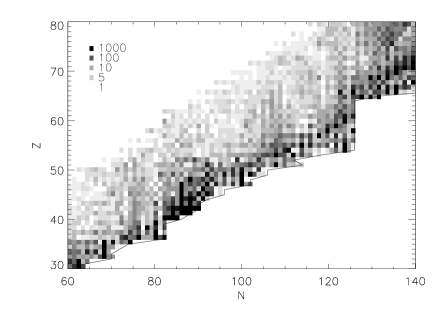
FIG. 8.: For each $N,Z$ the log of the ratio of the highest neutron-capture rate in our set [2, 10, 11, 12] to the lowest. The darkest squares correspond to ratios greater than 1000, as indicated in the key.

FIG. 9.: The four sets of neutron-capture rates, plotted as a function of $Z$, for $N=124$ just below the closed neutron shell.

FIG. 10.: Abundance curves from our standard simulation with the 4 sets of neutron-capture rates. Faster rates near the closed shell yield a narrower $A=195$ peak (note the left edge of that peak).

We can see the role of capture near the peak even more clearly by changing the rates only for $N$ between 123 and 125. Fig. 11 shows the results when those rates are multiplied by 10 or 100, or divided by 100. When the rates increase, funneling becomes stronger and spreading weaker as $(n,\gamma)\leftrightarrow(\gamma,n)$ equilibrium is partially restored. As a result, the final abundance peak at $A=195$ narrows.

FIG. 11.: Abundance curve when the capture rates for $N=123-125$ alone are changed. The solid line represents the results of with the rates from ref. [2], the dotted line the results when those rates are increased by 10, the dashed line the results when the rates are increased by 100, and the dot-dashed line the results when the rates are shrunk by 100.

It so happens that the nuclei at and just below closed shells are notoriously difficult to calculate [13]. Commonly used statistical methods may not be applicable for all those nuclei because of the low density of states at low energies [13, 12]. Rates of direct capture, which also plays a role, are uncertain because we don’t know how much isovector dipole strength lies low in nuclei far from stability. To determine the astrophysical parameters in the $r$-process environment, it’s therefore important to measure the rates in these nuclei where possible. Of course most of them are out of experimental reach for a long time to come. But the most important are actually relatively close to stability.

To show why this is, we make even more selective changes, now for just 1 or 2 values of $Z$, in the rates for $N$ between 123 and 125. Fig. 12 plots the root-mean-square difference between the abundance distribution (within our standard simulation) when these rates are increased by 100 and and when they are unaltered, as a function of time. The ultimate degree of change depends strongly on which rates we change. Altering those below $Z=69$ does little in the end because a) these nuclei are farther from stability, where the system is closer to $(n,\gamma)\leftrightarrow(\gamma,n)$ equilibrium and capture rates are nearly irrelevant, and b) Any changes that do occur have time to be diluted by spreading. Altering those above $Z=72$ doesn’t do much to the final abundance pattern because the system has nearly frozen out of equilibrium, making neutron capture irrelevant because there are so few free neutrons and the temperature has dropped. The nuclei for which changes do have large permanent effects lie between $Z=69$ and 72 (Tm,Yb,Lu,and Hf), and correspond to the rough location of the path just before full freezeout, when neutron capture and beta decay compete on equal footing. Then dramatic differences in flow result from increasing the neutron-capture rates, differences that are not erased by subsequent spreading. We see similar effects when the rates are decreased instead of increased. Fig. 13 shows final abundance curve for a standard run with the rates of ref. [2] and standard runs in which the capture rates of the nuclei with $Z=69-72$ and $N=123-125$ are increased by 10 and 100. The differences are significant. All these statements remain true both when we make wide variations in the initial temperature, initial density, and time scale in our simulations, and when we use the conditions of ref. [5]. The reason is that in this range of $Z$, the calculated [9] beta-decay lifetimes of the $N=126$ nuclei increase from about .07 s to 4.2 s. The path there slows down around the peak, giving the neutrons time to disappear through capture on nuclei in other regions. This happens whether in the time prior the path moves over a large distance (quickly at first, because of the fast beta decay rates far from stability) or over a shorter distance. Although it’s theoretically possible for freezeout to occur for $Z<69$, the resulting peak would almost certainly be too low in $A$ to match the observed abundances.

FIG. 12.: Root-mean-square differences between the abundances with the rates of [2] and with those same rates everywhere except for a few nuclei with two values of $Z$ and $N=123-125$ (those are multiplied by 100), as a function of time. We used the standard-simulation conditions. Each curve corresponds to increasing a different set of rates. The nuclei with the largest effect on the final abundances have $Z=69-70$ and $71-72$.

FIG. 13.: Final abundance curves in the simulation yielding fig. 12 when only the rates of nuclei with $N=123-125$ and $Z=69-72$ are increased, by factors of 1 (solid line), 10 (dotted line) and 100 (dashed line). Note the results of these simulations are nearly identical to those of fig. 11; the largest changes to the final abundance distribution are due to the modification of the capture rates of just these four nuclei.

The rates for these few nuclei are thus the ones on which the final $r$-process abundances depend most sensitively, and measuring the associated cross sections would be useful; we could then better constrain the temperature and density during the $r$ process. Unfortunately these nuclei are still far enough from stability that their cross sections may not be possible to measure, even partially through spectroscopic factors in transfer reactions with radioactive beams at RIA. A yield of about $10^{4}$/sec is probably necessary for such experiments, while estimates [15] of production at a RIA ISOL facility indicate that $Z$ must be about 77 before yields will become that large. But we can approach the nuclei we’re interested in, and see how measurements and calculations compare near the most critical region.

We’re more fortunate in the rare-earth region because neutron-capture rates are faster there than near the $A=195$ peak, and freezeout therefore occurs closer to stability. Fig. 14 shows what happens when we selectively change the capture rates of nuclei just below the kink, with $N=102-104$, for particular values of $Z$. The nuclei with the strongest effect now have $Z=62$ and 63 (Sm and Eu). As before, the location of the most important nuclei is not very sensitive to initial $r$-process conditions. These nuclei are actually within RIA’s reach. For the nucleus $Z=62,N=102$ (¹⁶⁴Sm), yields should be about $10^{5}$/sec, for $Z=63,N=102$ (¹⁶⁵Eu) they should be about $10^{6}$/sec, and for $Z=63,N=104$ (¹⁶⁷Eu) about $10^{4}$/sec [15]. Experiments to study their capture cross sections are worth considering.

FIG. 14.: Same as fig. 12, except for the rare-earth region, where rates of nuclei with $N=102-104$ and particular values of $Z$ are changed. The nuclei with the largest effect on the final abundances have $Z=62-63$.

We have not discussed the $A=130$ peak in any detail. Our conclusions there are more limited because we do not reproduce the region below the peak very well. Abundances in that area are very sensitive to the outcome of the alpha process, which we do not simulate. Nonetheless we do get a peak at $A=130$ and generally find that varying the $N=79-81$ neutron-capture rates has the largest effect for $Z=48-51$ (^127-129Cd, ^128-130In, ^129-131Sn, ^130-132Sb). RIA should be able to make enough of these isotopes to allow experiments.

V Conclusion

For most of the $r$ process, neutron-capture rates are irrelevant because they are fast enough to maintain equilibrium with photodisintegration. But at late times, the situation is different. Our investigation of funneling and spreading led us to identify particular nuclei relatively close to stability whose neutron-capture rates have significant effects on the shapes of peaks. It would be nice to have experimental information about these nuclei, even if indirect, e.g. spectoscopic factors through $(d,p)$ neutron-transfer reactions. Measurements of the capture rates themselves in other nuclei closer to stability would also be useful; they would help tune models, which could then be better extrapolated to the important nuclei identified here. A full understanding of the $r$ process would then be a little closer.

We thank J.H. de Jesus, B.S. Meyer, M. Smith, and P. Tomasi for useful discussions. We were supported in part by the U.S. Department of Energy under grant DE–FG02–97ER41019.

REFERENCES

- [1] E. M. Burbidge, G. R. Burbidge, W. A. Fowler, and F. Hoyle, Rev. Mod. Phys. 29, 547 (1957).
- [2] J.J. Cowan, F.-K. Thielemann, and J. W. Truran, Phys. Rep. 208, 257 (1991) is a review.
- [3] B.S. Meyer, Ann. Rev. Astron. Astrophys. 32, 153 (1994) is another review.
- [4] Y.-Z. Qian and S.E. Woosley, Ap. J. 471, 1331 (1996); R.D. Hoffman, S.E. Woosley, and Y.-Z. Qian, Ap. J. 482, 951 (1997).
- [5] C. Freiburghaus et al., Ap. J. 516, 381 (1999).
- [6] R. Surman, J. Engel, J.R. Bennett, and B.S. Meyer, Phys. Rev. Lett. 79, 1809 (1997)
- [7] B.S. Meyer, G.J. Mathews, W.M. Howard, S.E. Woosley, and R. Hoffman, Astrophys. J. 399, 656 (1992).
- [8] P. Möller, J. R. Nix, W. D. Myers, and W. J. Swiatecki, At. Data Nucl. Data Tables 59, 185 (1995).
- [9] P. Möller, and J. Randrup, Nucl. Phys. A514, 1 (1990).
- [10] S. Goriely, unpublished.
-
[11]
Institut d’Astronomie et d’Astrophysique CP226,
Université
Libre de Bruxelles,
http://www-astro.ulb.ac.be/Html/ncap.html . -
[12]
T. Rauscher and F.-K. Thielemann, At. Data Nucl. Data
Tables 75, 1 (2000);
ftp://quasar.physik.unibas.ch/pub/tommy/astro/fits/
957fit_frdm.asc.gz . - [13] see S. Goriely, Phys. Lett. B436, 10 (1998), Astr. Astrophys. 325, 414 (1997).
- [14] J. Engel, M. Bender, J. Dobaczewski, W. Nazarewicz, and R. Surman, Phys. Rev. C60 (1999) 14302.
-
[15]
See the RIA web page
http://www.phy.anl.gov/ria/index.html .