Non-local kinetic simulation of heavy ion collisions

Abstract

The numerical solutions of nonlocal and local Boltzmann kinetic equations for the simulation of peripheral and central heavy ion reactions are compared. The experimental finding of enhancement of mid-rapidity matter shows the necessity to include nonlocal corrections. While the in–medium cross section changes the number of collisions and not the transferred energy, the nonlocal scenario changes the energy transferred during collisions. The renormalisation of quasiparticle energies by using the Pauli–rejected collisions leads to a further enhancement of mid–rapidity matter distribution and is accompanied by a dynamical softening of the equation of state.

The simulation results are parameterised in terms of time dependent thermodynamical variables in the Fermi liquid sense. This allows one to discuss dynamical trajectories in phase space. A combination of thermodynamical observables is constructed which locates instabilities and points of possible phase transition under iso-nothing conditions. Two different mechanisms of instability, a short time surface–dominated instability and later a spinodal–dominated volume instability is found. The latter one occurs only if the incident energies do not exceed significantly the Fermi energy and might be attributed to spinodal decomposition.

1 Introduction

The formation of a neck–like structure in peripheral heavy ion reactions and the impact on the fragmentation mechanism and production of light charged particles has been discussed for a couple of years [1]- [2]. Theoretical investigations suggest that the neck is not formed in usual heavy ion simulations starting from the Landau equation [3, 4, 5] or BUU equations [6, 7] including additional mean field fluctuations derived in [8, 9] and tested [10]. The inclusion of fluctuations in the Boltzmann (BUU) equation has been investigated resulting in Boltzmann-Langevin pictures [11, 12, 13]- [14].

We will take here the point of view that the fluctuations should arise by themselves in a proper kinetic description where all relevant correlations are included in the collision integral. The collision will then cause both a dephasing and fluctuation by itself. This procedure without additional assumption about fluctuations has been given by the nonlocal kinetic theory [15, 16, 17] and applied to heavy ion collisions in [18]- [19]. We claim that the derived nonlocal off-set in the collision procedure induces fluctuations in the density and consequently in the mean-field which are similar to the one assumed in Boltzmann Langevin approaches above.

Recent INDRA observation shows an enhancement of emitted matter in the region of almost zero relative velocity which means that matter is stopped during the reaction and stays almost at rest [20, 21, 22, 23]. This enhancement of mid–rapidity distribution can possibly be associated with a pronounced neck formation of matter.

We use for the description the nonlocal kinetic equation [15, 24] for the one - particle distribution function

$${\partial f_{1}\over\partial t}+{\partial\varepsilon_{1}\over\partial{\bf k}}{\partial f_{1}\over\partial{\bf r}}-{\partial\varepsilon_{1}\over\partial{\bf r}}{\partial f_{1}\over\partial{\bf k}}=\sum_{b}\int{d{\bf p}d{\bf q}\over(2\pi)^{5}\hbar^{7}}\delta\left(\varepsilon_{1}+\varepsilon_{2}-\varepsilon_{3}-\varepsilon_{4}+2\Delta_{E}\right)\left|{\cal T}_{ab}\right|^{2}=$$

$$\Bigl{[}f_{3}f_{4}\bigl{(}1-f_{1}\bigr{)}\bigl{(}1-f_{2}\bigr{)}-\bigl{(}1-f_{3}\bigr{)}\bigl{(}1-f_{4}\bigr{)}f_{1}f_{2}\Bigr{]},$$ (1)

with Enskog-type shifts of arguments [15, 24]: $f_{1}\equiv f_{a}({\bf k,r},t)$, $f_{2}\equiv f_{b}({\bf p,r}\!-\!\Delta_{2},t)$, $f_{3}\equiv f_{a}({\bf k\!-\!q}\!-\!\Delta_{K},{\bf r}\!-\!\Delta_{3},t\!-\!\Delta_{t})$ , and $f_{4}\equiv f_{b}({\bf p\!+\!q}\!-\!\Delta_{K},{\bf r}\!-\!\Delta_{4},t\!-\!\Delta_{t})$ . The effective scattering measure, the ${\cal T}$-matrix is centred in all shifts. The quasiparticle energy $\varepsilon$ contains the mean field as well as the correlated self energy. In agreement with [25, 26], all gradient corrections are given by derivatives of the scattering phase shift $\phi={\rm Im\ ln}{\cal T}^{R}_{ab}(\Omega,{\bf k,p,q,}t,{\bf r})$,

$$\begin{array}[]{lclrclrcl}\Delta_{2}&=&{\displaystyle\left({\partial\phi\over\partial{\bf p}}-{\partial\phi\over\partial{\bf q}}-{\partial\phi\over\partial{\bf k}}\right)_{\varepsilon_{3}+\varepsilon_{4}}}&\ \ \Delta_{3}&=&{\displaystyle\left.-{\partial\phi\over\partial{\bf k}}\right|_{\varepsilon_{3}+\varepsilon_{4}}}&\ \ \Delta_{4}&=&{\displaystyle-\left({\partial\phi\over\partial{\bf k}}+{\partial\phi\over\partial{\bf q}}\right)_{\varepsilon_{3}+\varepsilon_{4}}}\\ &&&&&&&&\\ \Delta_{t}&=&{\displaystyle\left.{\partial\phi\over\partial\Omega}\right|_{\varepsilon_{3}+\varepsilon_{4}}}&\ \ \Delta_{E}&=&{\displaystyle\left.-{1\over 2}{\partial\phi\over\partial t}\right|_{\varepsilon_{3}+\varepsilon_{4}}}&\ \ \Delta_{K}&=&{\displaystyle\left.{1\over 2}{\partial\phi\over\partial{\bf r}}\right|_{\varepsilon_{3}+\varepsilon_{4}}}.\end{array}$$ (2)

After derivatives, $\Delta$’s are evaluated at the energy shell $\Omega\to\varepsilon_{3}+\varepsilon_{4}$. Neglecting these shifts the usual BUU scenario appears. The scattering integral of the non-local kinetic equation derived in [15, 24] corresponds to the picture of a collision as seen in Figure 1.

Figure 1: A nonlocal binary collision according to Eq. (1). Here $\Delta^{\rm be}=\Delta_{2}$, $\Delta_{a}=\Delta_{3}$ and $\Delta_{b}=\Delta_{4}-\Delta_{2}$ is used.

Despite its complicated form it is possible to solve this kinetic equation with standard Boltzmann numerical codes and to implement the shifts [16, 27, 19]. To this end we have calculated the shifts for different realistic nuclear potentials [18]. These shifts and the modifications of standard BUU or QMD code are available from the author. The numerical solution of the nonlocal kinetic equation has shown an observable effect in the dynamical particle spectra [16] as well as in the charge density distribution [19]. The high energetic tails of the spectrum are enhanced due to more energetic two-particle collisions in the early phase of nuclear collision. Therefore the nonlocal corrections lead to an enhanced production of preequilibrium high energetic particles.

Besides the nonlocal shifts and cross section which has been calculated from realistic potentials, the interaction affects, however, the free motion of particles between individual collisions. The dominant effect is due to mean-field forces which bind the nucleus together, accelerating particles close to the surface towards the centre. These mean-field forces are conveniently included via potentials of Skyrme type

$$\varepsilon={p^{2}\over 2m}+A\left({n\over n_{0}}\right)+B\left({n\over n_{0}}\right)^{\sigma}.$$ (3)

For a derivation of collision integrals and the Skyrme potential (3) from the same microscopic footing, see [28].

Beside forces, the interaction also modifies the velocity with which a particle of a given momentum propagates in the system. This effect is known as the mass renormalisation. A numerical implementation of the renormalised mass is rather involved since a plain use of the renormalised mass instead of the free one leads to incorrect currents. Within the Landau concept of quasiparticles, this problem is cured by the back flow, but it is not obvious how to implement the back flow within the BUU simulation scheme. In our studies, we circumvent the problem of back flows using explicit zero-angle collisions to which we add a non-local correction. One can show that indeed the non-local shifts create just the dynamical mass renormalisation if used for the Pauli-rejected events. The incorporation of a nonlocal jump without performing finite angle collisions for such events correspond exactly to the quasiparticle and dynamical mass renormalisation [19].

Finally, we would like to comment on properties of the proposed simulation scheme. The renormalisation depends on the distribution of particles in surrounding medium. It has four nice properties: (i) the renormalisation vanishes as the local density goes to zero, (ii) the renormalisation vanishes when a high temperature closes the Luttinger gap because all collisions will be at finite angles, (iii) the anisotropy of the quasiparticle velocity in a presence of a non-zero current in medium is automatically covered, and (iv) the backflows connected to the mass renormalisation are covered because both particles jump keeping the centre of mass fixed. Last but not least, the simulation does not require to introduce new time-demanding procedures, one can simply use the scattering events which are merely rejected in standard simulation codes by Pauli-blocking.

2 Numerical results

Let us discuss the proposed correction to the local and ideal (no quasiparticle renormalisation) Boltzmann (BUU) simulation. First we introduce the pure nonlocal corrections and then we discuss the quasiparticle renormalisation.

The evolution of the density can be seen in the corresponding left pictures of figure 2 for the BUU (left panel) and nonlocal scenario (middle panel) as well as the additional quasiparticle renormalisation (right panel). We see that the nonlocal scenario leads to a longer and more pronounced neck formation between $200-240$fm/c while the BUU breaks apart already at $200$fm/c.

Figure 2: First part.

Figure 2: The time evolution of ${}^{181}_{73}Ta+^{197}_{79}Au$ collisions at $E_{lab}/A=33$ MeV and $8$ fm impact parameter in the local BUU (left), non-local BUU (middle), and the non-local BUU with quasiparticle renormalisation (right). Plots in the first column show the $(x-z)$-density cut of $30$ fm$\times 30$ fm where $Ta$ as projectile comes from below. The mass momenta are shown by arrows. The corresponding second columns give the charge density distribution versus relative velocity in $cm/ns$ where the target like distribution of $Au$ is on the left and the projectile like distributions of $Ta$ on the right.

The question arises whether this pronounced neck formation and increase of mid-rapidity distribution is simply occurring by more collisions and corresponding correlations as called in–medium effect. This is however only the case for smaller impact parameters [22]. We see in the next figure 3 the number of collisions per time for the simulation where in the local BUU scenario the cross section has been doubled. The number of collisions is visibly enhanced by doubling the cross section while for the nonlocal scenario we get only a slight enhancement at the beginning and later even lower values with respect to local BUU. The latter fact comes from the earlier decomposition of matter in the nonlocal scenario.

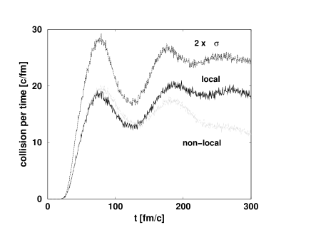
Figure 3: The time evolution of the number of nucleon collisions for $Ta+Au$ at $E_{lab}/A=33$ MeV and different impact parameter in the BUU (thick black line), non-local kinetic model (broken line) and the local BUU with a doubled cross section (thin dark line). The impact parameter is 8 fm.

The corresponding transverse and kinetic energies in figure 4 ($8$fm impact parameter) show that the transverse and longitudinal energy is almost not changed compared with local BUU. Oppositely the nonlocal scenario leads to an increase of transverse energy of about $2$MeV and about $1$MeV in longitudinal energy. We conclude that the increase of cross section leads to a higher number of collisions but not to more dissipated energy while the nonlocal scenario does not change the number of collisions much but the energy dissipated during the collisions. Returning to the discussion of pronounced neck formation in figure 2 above we see now that the quality rather than the quantity of collisions is what produces the neck.

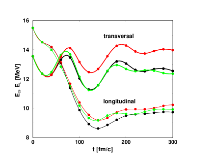
Figure 4: The time evolution of the longitudinal (thin lines) and transverse energy (thick lines) including Fermi motion of nucleon collisions for $Ta+Au$ at $E_{lab}/A=33$ MeV in the BUU (black line), nonlocal kinetic equation (light line) and the local BUU but with twice the cross section (medium line).

Now we can proceed and discuss the charge matter distribution with respect to the velocity. We plotted in figure 2 also the normalised charge distribution versus velocity and see that after $160$fm/c we have an appreciable higher mid–rapidity distribution for the nonlocal scenario (mid panel) than the BUU (left panel). Together with the observation that for nonlocal scenario we have a pronounced neck formation we see indeed that the neck formation is accompanied with high mid-velocity distribution of matter. We see in figure 2 (right panel) that the mid–rapidity distribution of matter is once more enhanced for quasiparticle renormalisation in comparison to the nonlocal scenario without quasiparticle renormalisation. The detailed comparison of the time evolutions of the transverse energy for $8$fm impact parameter can be seen in figure 5.

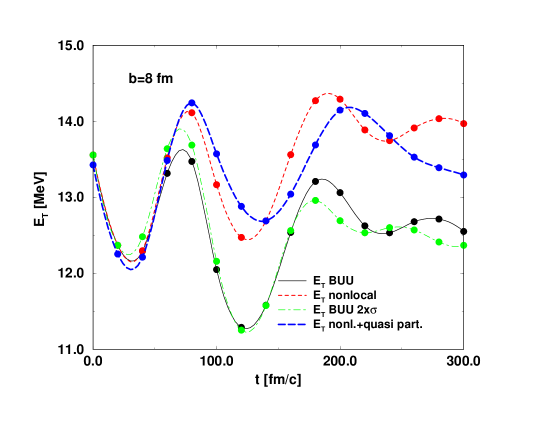
Figure 5: The time evolution of the transverse energy including Fermi motion for $Ta+Au$ at $E_{lab}/A=33$ MeV and $8$fm impact parameter in the BUU (black line), nonlocal kinetic equation (dashed line), the local BUU but twice cross section (dashed dotted line) and the nonlocal scenario with quasiparticle renormalisation (long dashed line).

We recognise that the transverse energies including quasiparticle renormalisation are similar to the nonlocal scenario and higher than the BUU or BUU with twice the cross section. However please remark that the period of oscillation in the transverse energy which corresponds to a giant resonance becomes larger for the case with quasiparticle renormalisation. Since therefore the energy of this resonance decreases we can conclude that the (nuclear) compressibility has been decreased by the quasiparticle renormalisation. Sometimes this quasiparticle renormalisation has been introduced by momentum dependent mean-fields. The effect is known to soften the equation of state. We see here that we get a dynamical quasiparticle renormalisation and a softening of equation of state. This softening of equation of state is already slightly remarkable when the nonlocal scenario is compared with BUU. With additional quasiparticle renormalisation we see that this is much pronounced.

We want to repeat that the dynamical quasiparticle renormalisation which leads to a softening of the equation of state enhances the mid rapidity distribution. In contrast a mere soft static parametrisation of the mean-field does not change the mid-rapidity emission appreciably [22].

2.1 Comparison with experiments

The BUU simulations will now be compared to one experiment performed with INDRA at GANIL, the $Ta+Au$ collision at $E_{lab}/A=33$ MeV.

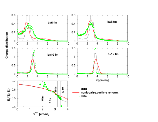
Figure 6: The experimental charge distribution of matter (dotted line) versus velocity in comparison within the BUU (thin solid line) and the nonlocal model with quasiparticle renormalisation (thick line). The maximum velocity versus ratio of longitudinal to total kinetic energy of $Ta+Au$ collisions at $E_{lab}/A=33$ MeV is given below. The selected experimental cuts are given by dots.

For the identification with experimental data we select events which show a clear one fragment structure. This correspond to events where we have clear target and projectile like residues. Since the used kinetic theory is not capable to describe dynamical fragment formation we believe that these events are the ones which are at least describable within our frame. Next we use impact parameter cuts with respect to the transverse energy since this shows in all simulations a fairly good correlation to the impact parameter. In our numerical results we see almost linear correlations between impact parameter, maximal velocity and the convenient ratio between transverse and total kinetic energy as seen in figure 6.

For each selected experimental transverse energy bin we can plot now the maximum velocity versus the ratio of the transverse to kinetic energy. We see in figure 6 that the numerical velocity damping agrees with the experimental selection only for very peripheral collisions. For such events we plot in the figure 6 the charge density distribution and compare the experiment with the simulation. These charge density distributions have been obtained using the procedure described in reference [23]. The Data are represented by light grey points, the standard BUU calculation by the thin line and the non-local BUU with quasiparticle renormalisation calculation by the thick line. A reasonable agreement is found for the nonlocal scenario including quasiparticle renormalisation while simple BUU fails to reproduce mid–rapidity matter.

3 Nonequilibrium Thermodynamics

In order to understand the different thermodynamics induced by nonlocal corrections and therefore virial correlations, we multiply the kinetic equation with $1,{\bf p},\varepsilon$ and obtain the balance for the particle density $n$, the momentum density $J$ and the energy density ${\cal E}$, see details in [27]. Please note that besides the mean field (3) we have also a Born correlation term, see [29, 28],

The correlational parts of the density, pressure and energy are arising from genuine two-particle correlations beyond Born approximation which are also derived from the balance equations of nonlocal kinetic equations [15, 24]. It has been shown that they establish the complete conservation laws. While these correlated parts are present in the numerical results and can be shown to contribute to the conservation laws we will only discuss the thermodynamical properties in terms of quasiparticle quantities to compare as close as possible with the mean field or local BUU expressions. The discussion of these correlated two - particle quantities is devoted to a separate consideration.

From the distribution function $f({\bf p,r},t)$ the local density, current and energy densities are given by

$$\left(\matrix{{n}({\bf r},t)\cr{\bf J}({\bf r},t)\cr{\cal E}_{K}({\bf r},t)}\right) = \int{d{\bf p}\over(2\pi\hbar)^{3}}\left(\matrix{1\cr{\bf p}\cr{p^{2}/2m}}\right){f({\bf p,r},t)}$$ (4)

which are computed directly from the numerical solution of the kinetic equation in terms of test particles. Please note that the above kinetic energy includes the Fermi motion.

The global variables per particle number like kinetic energy, Fermi energy and collective energy are obtained by spatial integration

$$\left(\matrix{{\cal E}_{K}(t)\cr{\cal E}_{F}(t)\cr{\cal E}_{\rm coll}(t)}\right) = \int d{\bf r}\left(\matrix{{\cal E}_{K}({\bf r},t)\cr{\cal E}_{f}[{n}({\bf r},t)]{n}({\bf r},t)\cr{{J}({\bf r},t)^{2}/m\,{n}({\bf r},t)}}\right){/\int d{\bf r}\,{n}({\bf r},t)}$$ (5)

where we have used the local density approximation [30]. Now we adopt the picture of Fermi liquid theory which connects the temperature with the kinetic energy as

$${\cal E}_{K}(t)=\frac{3}{5}{\cal E}_{F}(t)+{\cal E}_{\rm coll}(t)+{\pi^{2}\over 4{\cal E}_{F}(t)}{T(t)}^{2}$$ (6)

from which we deduce the global temperature. The definition of temperature is by no means obvious since it is in principle an equilibrium quantity. One has several possibilities to define a time dependent equivalent temperature which should approach the equilibrium value when the system approaches equilibrium. In [31, 32] the definition of slope temperatures has been discussed and compared to local space dependent temperature fits of the distribution function of matter. This seems to be a good measure for higher energetic collisions in the relativistic regime. Since we restrict us here to collisions in the Fermi energy domain and do not want to add coalescence models we will not use the slope temperature. Moreover we define the global temperature in terms of global energies which are obtained by local quantities rather than by defining a local temperature itself. This has the advantage that we do not consider local energy fluctuations but only a mean evolution of temperature.

The mean field part of the energy is given by

$$U(t) = {\cal E}^{\rm qp}(t)-{\cal E}_{K}(t)-{\cal E}^{\rm Born}(t)={\displaystyle{\int d{\bf r}\left(A{{n({\bf r},t)}^{2}\over 2n_{0}}+B{{n({\bf r},t)}^{s+1}\over(s+1)n_{0}^{s}}\right)}/\displaystyle{\int d{\bf r}\,{n}({\bf r},t)}}$$ (7)

from which one deduces the pressure per particle

$$P(t) = \frac{2}{3}({\cal E}_{K}(t)-{\cal E}_{\rm coll}(t))+\frac{4}{3}{\cal E}^{\rm Born}(t)+{\displaystyle{\int d{\bf r}\left(A{{n({\bf r},t)}\over 2n_{0}}+B{s\,{n({\bf r},t)}^{s}\over(s+1)n_{0}^{s}}\right)}/\displaystyle{\int d{\bf r}\,{n}({\bf r},t)}}.$$ (8)

In order to compare now the local BUU with the nonlocal BUU scenario we consider the energy which would be the total energy in the local BUU without Coulomb energy

$${\cal E}(t)={\cal E}_{K}(t)-{\cal E}_{\rm coll}(t)+U(t).$$ (9)

This expression does not contain the two - particle correlation energy which is zero for BUU and the Coulomb energy. The reason for considering this energy for dynamical trajectories is that we want to follow the trajectories in the picture of mean field and usual spinodal plots.

To define the density exhibits to some extend a problem. Depending on the considered volume sphere we obtain different global densities. We follow here the point of view that the mean square radius will be used as a sphere to define the global density. This is also supported by the observation that the mean square radius follows the visible compression.

3.1 Iso-nothing conditions in equilibrium

Let us first recall the figures of mean field isotherms in equilibrium. We obtain the typical van der Waals curves in figure 7. Since we have neither isothermal nor isochoric nor isobaric conditions in simulations, shortly since we have iso-nothing conditions, we have to find a representation of the phase transition curves which are independent of temperature but which reflect the main features of phase transitions. This can be achieved by the product of energy and pressure density versus energy density in figure 7 below. This plot shows that all instable isotherms exhibit a minimum in the left lower quarter. There the energy is negative denoting bound state conditions but the pressure is already positive which means the system is unstable. The first isotherm above the critical one does not touch this quarter but remains in the right upper quarter where the energy and pressure are both positive and the system is expanding and decomposing unboundly. The left upper quarter denotes negative pressure and energy indicating that the system is bound and stable.

In order to achieve now a temperature independent plot we scale both axes of figure 7 (below) with a temperature dependent polynomial and achieve that all critical isotherms are collapsing on one curve in the left lower quarter. The first isotherms above the critical one does not enter the left lower quarter. We consider this scaling as adequate for iso-nothing conditions. A phase transition should be possible to observe if there occurs a minimum in the left half of this plot at negative energies.

Figure 7: The isotherms for the pressure density versus volume and for the product of pressure and energy density versus energy density (above). The temperatures are $T=1,4,7,10,13,16,19$MeV. The isotherms of the product of pressure and energy density versus energy density scaled by a temperature polynomial $f(T)$, $g(T)$ (below). All critical isotherms collapse on one line in the left lower quarter.

The idea of plotting combinations of pressure and energy is similar to the one of softest point [33] in analysing QCD phase transitions. There the simple pressure over energy ratio leads to a temperature independent plot due to ultrarelativistic energy - temperature relations. In our case we have a Fermi liquid behaviour at low temperatures and the scaling temperature dependent polynomials, $f$ and $g$, can be found in [27] which are producing a temperature independent plot in figure 7.

3.2 Simulation results

Let us now inspect the dynamical trajectories for the above defined temperature, density and energy. In figure 8 we have plotted the dynamical trajectories for a charge - symmetric reaction of $Xe$ on $Sn$ at $25$MeV lab - energy. The solution of the nonlocal kinetic equation is compared to the local BUU one. One sees in the temperature versus density plane that the point of highest compression is reached around $60$fm/c with a temperature of $9$ MeV.

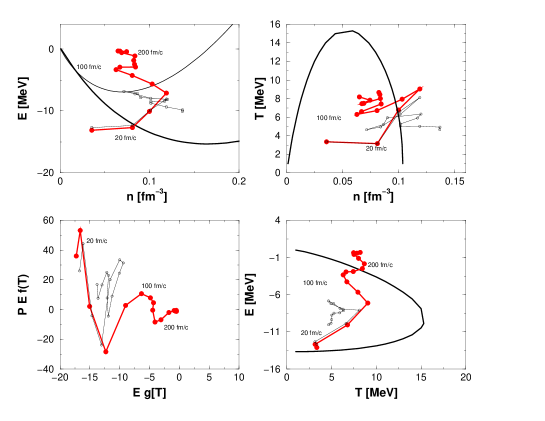
Figure 8: The dynamical trajectories of the energy (9), density and temperature (i6) in the nonlocal (gray thick) and in the local BUU (black thin) scenario. The considered reaction is ${}^{129}Xe$ on ${}^{119}Sn$ at $25$MeV lab energy. The dots mark the times in steps of $20$fm/c up to total of $300$fm/c. To guide the eye the zero temperature mean field energy (thick line) and the pressure (thin line) is plotted in the upper left picture and in the right figures the spinodal line for infinite matter is given. The scaled combinational plot analogous to figure 7 is given in the left lower plane.

After this point of highest overlap or fusion phase we have an expansion phase where the density and temperature is decreasing. While the compression phase is developing similar for the BUU and for the nonlocal kinetic equation we see now differences in the development. First the temperature of the nonlocal kinetic equation is around $2$MeV higher than the local BUU result. This is due to the release of correlation energy into kinetic energy which is not present in the local BUU scenario. After this expansion stage until times of $120$fm/c we see that the BUU trajectories come to a rest inside the spinodal region while the nonlocal scenario leads to a further decay. This can be seen by the continuous decrease of density and increase of energy. Since matter is more decomposed with the nonlocal kinetic equation we also heat the system more due to Coulomb acceleration. This leads to the enhancement of temperature compared to BUU. An oscillating behaviour occurs at later times which reflects an interplay between short range correlation and long range Coulomb repulsion. The decomposition leads almost to free gaseous matter after $300$fm/c as can be seen in the energy versus density plot.

Please note that although the trajectories seem to equilibrate inside the spinodal region when one considers the temperature versus density plane, we see that in the corresponding energy versus temperature plane the trajectories travel already outside the spinodal region. This underlines the importance to investigate the region of spinodal decomposition in terms of a three dimensional plot instead of a two dimensional one like in the recently discussed caloric curve plots. Different experimental situations lead to different curves as long as the third coordinate (pressure or density) remains undetermined.

The iso-nothing plot analogous to the left lower plot of figure 7 shows that the point of highest compression is linked to a first instability seen as a pronounced minimum of the trajectory in the left quarter. If we do not exceed the Fermi energy domain, this is connected with a pronounced surface emission and connected with anomalous velocity profiles [34]. We will call this phase surface emission instability further on. At $180$ fm/c we see a second minimum which is taking place inside the spinodal region. This instability we might now attribute to spinodal decomposition since the trajectories developing slower and remain inside the spinodal region. The BUU shows the same qualitative minima but the matter rebounds and the trajectories move towards negative energies again. In opposition the nonlocal scenario leads to a further decomposition of matter as described above.

In the next figure 9 we have plotted the same reaction as in figure 8 but at higher energy of $33$MeV. We recognise a higher compression density and temperature than compared to the lower bombarding energy. Consequently the trajectories develop further towards the unbound region of positive energy after $300$fm/c. While the first surface emission instability is strongly pronounced we see that the second minimum in the iso-nothing plot is already weaker indicating that the role of spinodal decomposition is diminished. The trajectories in the temperature versus density plot come still in the spinodal region at rest but travel already outside the spinodal region if the energy versus temperature plot is considered. This shows that the trajectories start to develop too fast to suffer much spinodal decomposition. Oppositely, at energies around the Fermi energy spinodal decomposition might be possible and is presumably connected with anomalous velocity and density profiles [34].

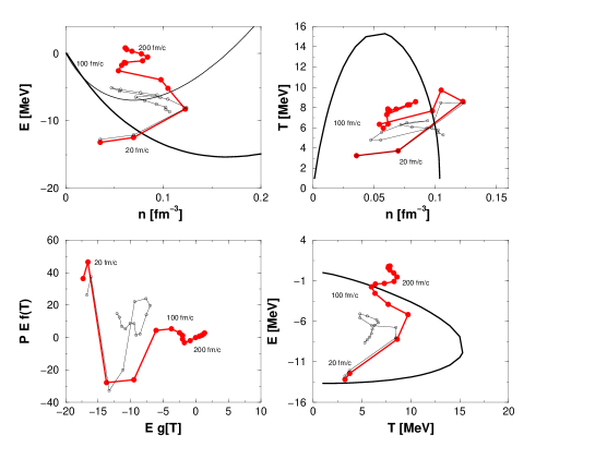
Figure 9: The same figure as 8 but for $33$MeV lab energy.

If we now plot the same reaction at $50$MeV in figure 10 we see that the trajectories come at rest outside the spinodal region whatever plot is used and no second minima is seen anymore in the iso-nothing plot. But, the surface emission instability is still very pronounced and is probably here the leading mechanism of matter disintegration.

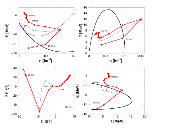
Figure 10: The same figure as 8 but for $50$MeV lab energy.

We might now search for a situation where we have the opposite extreme that is we search for a reaction with as less as possible surface emission instability and as much as possible spinodal decomposition. For this reason we might think on asymmetric reactions since the different sizes of the colliding nuclei might suppress the surface emission. Indeed as can be seen in figure 11 for an asymmetric reaction of $Ni$ on $Au$ at $25$MeV lab-energy with nearly the same total charge as in the reaction before that the surface emission instability is less pronounced while the spinodal instability is much more important. There appears even a third minima showing that the matter suffers spinodal decomposition perhaps more than once if the bombarding energy is low enough and a long oscillating piece of matter is developing.

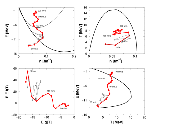
Figure 11: The same dynamical trajectories as in figure (8) but for a reaction ${}^{56}Ni$ on ${}^{179}Au$ at $25$MeV lab energy.

The higher bombarding energies now show the same qualitative effect which pronounces the surface emission instability and reduces the importance of the spinodal decomposition. Much smaller compression densities and temperatures are reached in these reactions compared to the more symmetric case of $Xe$ on $Sn$.

4 Summary

The extension of BUU simulations by nonlocal shifts and quasiparticle renormalisation has been presented and compared to recent experimental data on mid rapidity charge distributions. It is found that both the nonlocal shifts as well as the quasiparticle renormalisation must be included in order to get the observed mid–rapidity matter enhancement.

The inclusion of quasiparticle renormalisation has been performed by using the normally excluded events by Pauli blocking. Since the quasiparticle renormalisation and corresponding effective mass features can be considered as zero angle collisions they can be realized by nonlocal shifts for the scattering events which are normally rejected. This means that one has to perform the advection step for the cases of Pauli blocked collisions without colliding the particles. Besides giving a better description of experiments, this has the effect of a dynamically softening of equation of state seen in longer oscillations of giant compressional resonance.

In this way we present a combined picture including nonlocal off-sets representing the nonlocal character of scattering, which leads to virial correlations with the quasiparticle renormalisation, and as a result to mean field fluctuations. We propose that no additional stochasticity need to be assumed in order to get realistic fluctuations.

The nonlocal kinetic theory leads to a different nonequilibrium thermodynamics compared to the local BUU. We see basically a higher energetic particle spectra and a higher transversal temperature of $2$MeV. This is attributed to the conversion of two-particle correlation energy into kinetic energy which is of course absent in local BUU scenario.

By constructing a temperature independent combination of thermodynamical variables we are able to investigate the signals of phase transitions under iso-nothing conditions. Two mechanisms of instability have been identified: surface emission instability and spinodal decomposition. We predict for the currently investigated reactions seen in table 1 which effect should be the leading one for matter decomposition.

MeV 25 33 50 ${}^{58}_{28}$Ni + ${}^{197}_{79}$Au S CS C(S) ${}^{129}_{54}$Xe + ${}^{119}_{50}$Sn CS C(S) C MeV 15 33 60 ${}^{157}_{64}$Gd + ${}^{238}_{92}$U – CS C ${}^{181}_{73}$Ta + ${}^{197}_{79}$Au CS C(S) C

Table 1: The prediction of the leading mechanisms of matter disintegration for two reactions with equal total charge but symmetric and asymmetric entrance channels. Surface compression is denoted by $C$ and spinodal decomposition by $S$.

In the reactions with bombarding energies higher than the Fermi energy the fast surface eruption happens outside the spinodal region. For even higher energies there is not enough time for the system to rest at the spinodal region. The trajectories simply move through the spinodal and the system decays before it comes to an equilibrium - like state inside the spinodal region. Around the Fermi energy the spinodal decomposition might occur and is accompanied by an anomalous velocity and density profile [34].

5 Acknowledgements

The authors would like to thank the members of the INDRA collaboration for providing the experimental data.

References

- [1] L. Stuttgé and et al., Nucl. Phys. A 539, 511 (1992).
- [2] L. G. Sobotka, J. F. Dempsey, R. J. Charity, and P. Danielewicz, Phys. Rev. C 55, 2109 (1997).
- [3] C. Pethik and D. Ravenhall, Nucl. Phys. A 471, 19c (1987).
- [4] R. Donangelo, C. O. Dorso, and H. D. Marta, Phys. Lett. B 263, 19 (1991).
- [5] R. Donangelo, A. Romanelli, and A. C. S. Schifino, Phys. Lett. B 263, 342 (1991).
- [6] D. Kiderlen and H. Hofmann, Phys. Lett. B 332, 8 (1994).
- [7] S. Ayik, M. Colonna, and P. Chomaz, Phys. Lett. B 353, 417 (1995).
- [8] R. Balian and M. Veneroni, Ann. of Phys. 164, 334 (1985).
- [9] H. Flocard, Ann. of Phys. 191, 382 (1989).
- [10] T. Troudet and D. Vautherin, Phys. Rev. C 31, 278 (1985).
- [11] M. Colonna, M. DiToro, and A. Guarnera, Nucl. Phys. A 589, 160 (1995).
- [12] M. Colonna et al., Nucl. Phys. A 642, 449 (1998).
- [13] G. Fabbri, M. Colonna, and M. DiToro, Phys. Rev. C 58, 3508 (1998).
- [14] G. F. Burgio, P. Chomaz, and J. Randrup, Nucl. Phys. A 529, 157 (1991).
- [15] V. Špička, P. Lipavský, and K. Morawetz, Phys. Lett. A 240, 160 (1998).
- [16] K. Morawetz et al., Phys. Rev. Lett. 82, 3767 (1999).
- [17] P. Lipavský, V. Špička, and K. Morawetz, Phys. Rev. E 59, R 1291 (1999).
- [18] K. Morawetz, P. Lipavský, V. Špička, and N. Kwong, Phys. Rev. C 59, 3052 (1999).
- [19] K. Morawetz et al., Phys. Rev. C 63, 034619 (2001).
- [20] F. Bocage and et al., Nucl. Phys. A 676, 391 (2000).
- [21] E. Plagnol and et al., Phys. Rev. C 61, 014606 (2000).
- [22] E. Galichet, Ph.D. thesis, Insitut de Physique Nucléaire de Lyon, 1998.
- [23] J. F. Lecolley and et al., Nucl. Inst. and Meth. A 441, 517 (2000).
- [24] P. Lipavský, K. Morawetz, and V. Špička, (1999), book in press Annales de Physique, K. Morawetz, Habilitation University Rostock 1998.
- [25] P. J. Nacher, G. Tastevin, and F. Laloë, Ann. Phys. (Leipzig) 48, 149 (1991).
- [26] M. de Haan, Physica A 164, 373 (1990).
- [27] K. Morawetz, Phys. Rev. C 62, 44606 (2000).
- [28] K. Morawetz, Phys. Rev. C 63, 14609 63, 14609 (2001).
- [29] K. Morawetz and H. Köhler, Eur. Phys. J. A 4, 291 (1999).
- [30] P. Schuck et al., Prog. Part. Nucl. Phys. 22, 181 (1989).
- [31] T. Gaitanos, H. Wolter, and C. Fuchs, (2000), sub: nucl-th/0003043.
- [32] T. Gaitanos, H. Wolter, and C. Fuchs, Phys. Lett. B 478, 79 (2000).
- [33] C. M. Hung and E. V. Shuryak, Phys. Rev. Lett. 75, 4003 (1995).
- [34] K. Morawetz, S. Toneev, and M. Ploszajczak, Phys. Rev. C 62, 64602 (2000).