Self-consistent description of nuclear compressional modes

Abstract

Isoscalar monopole and dipole compressional modes are computed for a variety of closed-shell nuclei in a relativistic random-phase approximation to three different parametrizations of the Walecka model with scalar self-interactions. Particular emphasis is placed on the role of self-consistency which by itself, and with little else, guarantees the decoupling of the spurious isoscalar-dipole strength from the physical response and the conservation of the vector current. A powerful new relation is introduced to quantify the violation of the vector current in terms of various ground-state form-factors. For the isoscalar-dipole mode two distinct regions are clearly identified: (i) a high-energy component that is sensitive to the size of the nucleus and scales with the compressibility of the model and (ii) a low-energy component that is insensitivity to the nuclear compressibility. A fairly good description of both compressional modes is obtained by using a “soft” parametrization having a compression modulus of $K\!=\!224$ MeV.

I Introduction

The study of nuclear compressional modes, while interesting in its own right, is motivated by our desire to understand the equation of state of hadronic matter, especially in relation to its compression modulus. In turn, an accurate determination of the compression modulus places important constraints on theoretical models of nuclear structure, heavy-ion collisions, neutron stars, and supernovae explosions.

While it remains true that measuring the energy of the nuclear compressional modes provides the most accurate determination of the compression modulus, significant advances in astronomical observations and terrestrial experiments are providing important complimentary information. For example, explaining the time structure of the neutrino burst emitted from supernova SN1987A seems to require a relatively soft equation of state as input in the simulations of core-collapsed supernova [1, 2]. Further, the recently inferred narrow mass distribution of neutron stars [3] poses stringent constraints on the nuclear equation of state. At the same time, a number of improved radii-measurements of radio-quite, isolated neutron stars — such as RX J185635-3754 — will contribute significantly to our understanding of the high-density component of the equation of state [4]. Finally, measurements of the elliptical flow in relativistic heavy-ion reactions seem to have established the utility of this observable as a probe of the stiffness of the equation of state [5].

Also significant is the strong correlation between seemingly unrelated experiments. Indeed, the radius of a neutron star is predicted to be strongly correlated to the neutron skin of a heavy nucleus [6, 7]. Thus, the upcoming measurement of the neutron radius of ²⁰⁸Pb at the Jefferson Laboratory [8, 9] should place important limits on the radii of neutron-stars.

Although measurements of the giant monopole resonance [10, 11] and the isoscalar giant dipole resonance [12, 13, 14] have existed for some time, the field has seen a revitalization due to new and improved measurements of both compressional modes [15, 16, 17]. The field has also seen significant advances in the theoretical domain. Indeed, calculations of nuclear compressional modes using Hartree-Fock (HF) plus RPA approaches with state-of-the-art Skyrme interactions are now possible [18, 19]. Relativistic RPA models have also enjoyed a great deal of success, especially now that scalar self-interactions have been incorporated into the calculation of the response [20, 21, 22, 23]. At the same time the philosophy behind the theoretical extraction of the nuclear compressibility has evolved considerably. Earlier attempts depended heavily on semi-empirical formulas that related the compressibility to the energies of the compressional modes [24]. The field now demands stricter standards: the model, without any recourse to semi-empirical mass formulas, must predict both the compressibility of nuclear matter as well as the energy of the compressional modes.

In this publication state-of-the-art calculations of the isoscalar giant-monopole resonance (GMR) and the isoscalar giant-dipole resonance (ISGDR) are reported for a variety of closed-shell nuclei. This paper represents an expanded version of a short article published recently that focused exclusively on ²⁰⁸Pb [22]. The model adopted in this work is based on a relativistic random-phase-approximation (RPA) to three different parameterizations of the Walecka model with scalar self-interactions. A nonspectral approach that treats discrete and continuum excitations on equal footing is implemented. As a result, the conservation of the vector current is strictly maintained throughout the calculation. Moreover, for the calculation of the RPA response we employ a residual particle-hole interaction consistent with the particle-particle interaction used to generate the mean-field ground state. In this way the spurious isoscalar-dipole strength, associated with the uniform translation of the center-of-mass, gets shifted to zero excitation energy and is cleanly separated from the physical response.

Having established the theoretical underpinning of our calculation, it is now useful to contrast it against alternative self-consistent implementations. In a recent article by Shlomo and Sanzhur [25], it is suggested that actual implementations of the RPA, in spite of claiming otherwise, are not fully self-consistent. It is pointed out that these calculations often resort to a variety of approximations such as: (i) neglecting the two-body Coulomb and spin-orbit terms in the residual particle-hole interaction, (ii) approximating the momentum-dependent parts in the particle-hole interaction, (iii) limiting the particle-hole space in a discretized calculation by a cut-off energy $E_{ph}^{\rm max}$, and (iv) introducing a smearing parameter, such as a Lorentzian width. Each of these approximations is now briefly addressed. In the relativistic formalism employed here neither the two-body Coulomb nor the spin-orbit interaction are neglected. Rather, the residual particle-hole interaction includes the (isoscalar) contribution from the photon as well as spin-orbit effects that are incorporated — to all orders — by merely maintaining the relativistic structure of the interaction. Moreover, the residual particle-hole interaction is momentum independent because one preserves intact its full Lorentz structure; no momentum-dependence is generated through a nonrelativistic reduction of the interaction. Further, the non-spectral approach employed here avoids any reliance on artificial cutoffs and truncations. Finally, while a Lorentzian width is included to compute the properties of discrete excitations, it is done so by ensuring that the physically relevant quantities, the excitation energy and the inelastic form-factor, remain invariant under a change in width.

The paper has been organized as follows. Section II describes the relativistic mean-field plus RPA formalism in great detail placing special emphasis on the role of self-consistency. Section III illustrates the importance of self-consistency for the conservation of the vector current and for the decoupling of spurious strength from the physical isoscalar-dipole response. Here a powerful novel relation is introduced to quantify the violation of the vector current in terms of various known ground-state form-factors. Results are displayed in Sec. IV, while a summary and conclusions are presented in Sec. V.

II Formalism

In this section a detailed description of the mean-field plus RPA formalism employed to compute the distribution of strength for both compressional modes is presented. This formalism, with the exception of its implementation in the case of scalar self-interactions, has now been available for almost fifteen years [26, 27, 28]. However, important lessons keep being ignored [20], just to be soon rediscovered [21]. Thus, we feel compelled to present, for what we hope is the last time, a thorough discussion of the relativistic RPA formalism.

The first step in calculating a relativistic RPA response is the computation of the mean-field ground state in a self-consistent approximation. Once self-consistency is achieved, three important pieces of information become available: (i) the single-particle energies of the occupied orbitals, (ii) their single-particle wave functions, and (iii) the self-consistent mean-field potential. This mean-field potential, without any modification, must then be used to generate the nucleon propagator; in this way the conservation of the vector current is guaranteed to be maintained. The nucleon propagator is computed nonspectrally to avoid any dependence on the artificial cutoffs and truncations that plague most spectral approaches. Moreover, through a nonspectral approach one gives equal treatment to both bound and continuum orbitals.

Having generated the occupied single-particle spectrum and the nucleon propagator, the computation of the lowest-order (Hartree) polarization is reduced to the evaluation of various matrix elements of the relevant transition operator. To compute the RPA response one needs to go beyond the single-particle response. The RPA builds coherence among the many allowed particle-hole excitations by iterating the lowest-order polarization to all orders via the residual particle-hole interaction. Yet special care must be taken in adopting a residual particle-hole interaction consistent with the particle-particle interaction used to generate the mean-field ground state. Only then can one ensure that the spurious component of the isoscalar-dipole response will get shifted to zero excitation energy [29, 30]. As the polarization tensor is a fundamental many-body operator, it can be computed systematically using well-known many-body techniques [31]. Having computed the polarization tensor, the nuclear response is extracted by simply taking its imaginary part. The following sections provide a detailed account on the implementation of these ideas.

A The Lagrangian Density

The starting point for the calculation of the nuclear response is a Lagrangian density having an isodoublet nucleon field ($\psi$) interacting via the exchange of two isoscalar mesons, the scalar sigma ($\phi$) and the vector omega ($V^{\mu}$), one isovector meson, the rho ($b^{\mu}$), and the photon ($A^{\mu}$) [32, 33]. The pseudoscalar pion is not included as it does not contribute at the mean-field level. In addition to meson-nucleon interactions the Lagrangian density includes scalar self-interactions. These are responsible for reducing the nuclear compressibility from the unrealistically large value of $K\!=\!545$ MeV, obtained in the original linear model of Walecka [34], all the way down to the acceptable value of $K\!=\!224$ MeV. Thus, without the inclusion of scalar self-interactions a realistic calculation of the compressional modes is not feasible. The Lagrangian density for the model is thus given by

$${\cal L}_{\rm int}=\bar{\psi}\Big{[}g_{s}\phi-g_{\rm v}\hbox to0.0pt{/\hss}V-{g_{\rm\rho}\over 2}{\mbox{\boldmath$\tau$}}\cdot\hbox to0.0pt{/\hss}{\bf b}-{e\over 2}(1+\tau_{3})\,\hbox to0.0pt{/\hss}{\!A}\Big{]}\psi-U(\phi)\;;\quad U(\phi)=\frac{1}{3!}\kappa\phi^{3}+\frac{1}{4!}\lambda\phi^{4}\;,$$ (1)

were use of the“slash” notation, $\hbox to0.0pt{/\hss}V\!\equiv\gamma^{\mu}V_{\mu}$, has been made. The various model parameters have been listed in Table I.

B The nucleon propagator

The mean-field propagator contains information about the interaction of the propagating nucleon with the average potential generated by the nuclear medium. However, even in a Fermi-gas description, where all interactions are neglected, the nucleon propagator would still differ from its free-space value because of the presence of a filled Fermi sea. Indeed, the analytic structure of the free-nucleon propagator at finite density is different from its free-space value (see Fig. 1). This suggests the following decomposition of the nucleon propagator [32]:

$$G(x,y)=\int_{-\infty}^{\infty}{d\omega\over 2\pi}e^{-i\omega(x^{0}-y^{0})}G({\bf x},{\bf y};\omega)\;,$$ (3)

$$G({\bf x},{\bf y};\omega)=G_{F}({\bf x},{\bf y};\omega)+G_{D}({\bf x},{\bf y};\omega)\;.$$ (4)

The Feynman part of the propagator, $G_{F}$, admits a spectral decomposition in terms of the mean-field solutions to the Dirac equation. That is,

$$G_{F}({\bf x},{\bf y};\omega)=\sum_{n}\left[\frac{U_{n}({\bf x})\overline{U}_{n}({\bf y})}{\omega-E_{n}^{(+)}+i\eta}+\frac{V_{n}({\bf x})\overline{V}_{n}({\bf y})}{\omega+E_{n}^{(-)}-i\eta}\right]\;,$$ (5)

where $U_{n}$ and $V_{n}$ are the positive- and negative-energy solutions to the Dirac equation, and the sum is over all states in the spectrum. The analytic structure of $G_{F}$ is identical to that of the conventional Feynman propagator [35]. The density-dependent part of the propagator, $G_{D}$, corrects $G_{F}$ for the presence of a filled Fermi sea. This correction occurs even in a noninteracting system and is due to the Pauli exclusion principle. Formally, one effects this correction by shifting the position of the pole of every occupied state from below to above the real axis (see Fig. 1)

$$G_{D}({\bf x},{\bf y};\omega) = \sum_{n<{\rm F}}U_{n}({\bf x})\overline{U}_{n}({\bf y})\left[{1\over\omega-E_{n}^{(+)}-i\eta}-{1\over\omega-E_{n}^{(+)}+i\eta}\right]$$ (6)

$$= 2\pi i\sum_{n<{\rm F}}\delta\Big{(}\omega-E_{n}^{(+)}\Big{)}{U}_{n}({\bf x})\overline{U}_{n}({\bf y})\;.$$ (7)

Note that the sum over $n$ is now restricted to only those positive-energy states below the Fermi energy. In a mean-field approximation these states satisfy a Dirac equation of the form:

$$\left[E_{n}^{(+)}\gamma^{0}+i{\bf\gamma}\cdot{\bf\nabla}-M-\Sigma_{\rm MF}(x)\right]U_{n}({\bf x})=0\;,$$ (8)

where the mean-field potential is given by

$$\Sigma_{\rm MF}(x)=\Sigma_{\rm S}(x)+\gamma^{0}\Sigma_{0}(x)\;.$$ (9)

The quantities $\Sigma_{\rm S}$ and $\Sigma_{0}$ denote the scalar and vector potentials that have been generated self-consistently at the mean-field level. Since this work is limited to the response of closed-shell nuclei, it is assumed that the mean-field potential has been generated by a spherically-symmetric, spin-saturated ground state.

Although the above spectral decomposition of the nucleon propagator will become important in understanding the spectral content of the nuclear response, in practice it suffers from a reliance on artificial cutoffs and truncations. An efficient scheme that avoids such a dependence is the nonspectral approach. A nonspectral approach has the added advantage that both positive- and negative-energy continuua are treated exactly. As a result, the contributions from the negative-energy states to the response are included automatically. This is important to maintain fundamental physical principles, as the positive-energy states by themselves are not complete. To obtain the nucleon propagator in nonspectral form one must solve the following inhomogeneous Dirac equation:

$$\left[\omega\gamma^{0}+i{\bf\gamma}\cdot{\bf\nabla}-M-\Sigma_{\rm MF}(x)\right]G_{F}({\bf x},{\bf y};\omega)=\delta({\bf x}-{\bf y})\;.$$ (10)

Here $\omega$ is taken to be a complex variable and the mean-field potential is identical to the one used to generate the nuclear ground state. Taking advantage of the spherical symmetry of the potential, one may decompose the Feynman propagator in terms of spin-spherical harmonics

$$G_{F}({\bf x},{\bf y};\omega)=\frac{1}{xy}\sum_{\kappa m}\left(\matrix{\phantom{i}g_{11}^{\kappa}(x,y;\omega)\langle\hat{\bf x}|\!+\!\kappa m\rangle\langle+\kappa m|\hat{\bf y}\rangle&-ig_{12}^{\kappa}(x,y;\omega)\langle\hat{\bf x}|\!+\!\kappa m\rangle\langle-\kappa m|\hat{\bf y}\rangle\cr ig_{21}^{\kappa}(x,y;\omega)\langle\hat{\bf x}|\!-\!\kappa m\rangle\langle+\kappa m|\hat{\bf y}\rangle&\phantom{-i}g_{22}^{\kappa}(x,y;\omega)\langle\hat{\bf x}|\!-\!\kappa m\rangle\langle-\kappa m|\hat{\bf y}\rangle}\right)\;,$$ (11)

which are defined as

$$\langle\hat{\bf x}|\kappa m\rangle=\sum_{m_{l}m_{s}}\langle lm_{l},{\scriptstyle{\frac{1}{2}}}m_{s}|l{\scriptstyle{\frac{1}{2}}}jm\rangle Y_{lm_{l}}(\hat{\bf x})\chi_{{\scriptstyle{\frac{1}{2}}}m_{s}}\;,$$ (12)

$$\,j\!=\!|\kappa|\!-\!\frac{1}{2}\;\quad\hbox{and}\quad l=\cases{+\kappa&if $\kappa>0\;,$\cr-\kappa-1&if $\kappa<0\;.$}$$ (13)

The above decomposition enables one to rewrite the Dirac equation as a set of first-order, coupled, ordinary differential equations of the form

$$\left(\matrix{\omega^{*}\!-\!M^{*}&\displaystyle{\frac{d}{dx}\!-\!\frac{\kappa^{*}}{x}}\cr\displaystyle{\frac{d}{dx}\!+\!\frac{\kappa^{*}}{x}}&-\omega^{*}\!-\!M^{*}}\right)\left(\matrix{g_{11}^{\kappa}&g_{12}^{\kappa}\cr&\cr g_{21}^{\kappa}&g_{22}^{\kappa}}\right)=\delta(x-y)\;,$$ (14)

where we have defined

$$\omega^{*}\equiv\omega-\Sigma_{\rm v}(x)\;\hbox{and}\;\;\;M^{*}\equiv M+\Sigma_{\rm s}(x)\;.$$ (15)

It is important to underscore that the mean-field potentials used to compute the nucleon propagator must be identical to those used to generate the mean-field ground state if the conservation of the vector current is to be maintained.

C The nuclear polarization

To illustrate the many-body techniques employed in the manuscript, we define a general polarization insertion as the time-ordered product of two arbitrary nucleon currents:

$$i\Pi^{\alpha\beta}(x,y)=\langle\Psi_{0}|T\Big{[}\hat{J}^{\alpha}(x)\hat{J}^{\beta}(y)\Big{]}|\Psi_{0}\rangle\;,$$ (16)

where $\Psi_{0}$ denotes the exact nuclear ground state and $\hat{J}^{\alpha}(x)$ is a one-body current operator of the form

$$\hat{J}^{\alpha}(x)=\bar{\psi}(x)\Gamma^{\alpha}\psi(x)\;.$$ (17)

Note that the “big” gamma matrices have been defined so that the one-body current operator be hermitian [35]. That is,

$$\Gamma^{\alpha}=\{1,i\gamma^{5},\gamma^{\mu},\gamma^{\mu}\gamma^{5},\sigma^{\mu\nu}\}\quad{\rm with}\quad\overline{\Gamma}^{\alpha}\equiv\gamma^{0}\,\Gamma^{\alpha\dagger}\,\gamma^{0}=\Gamma^{\alpha}\;.$$ (18)

In a mean-field approximation to the nuclear ground state, such as the one employed here and in most of the other relativistic calculations to date, the polarization insertion may be written exclusively in terms of the nucleon mean-field propagator

$$i\Pi^{\alpha\beta}(x,y)={\rm Tr}\Big{[}\Gamma^{\alpha}G(x,y)\Gamma^{\beta}G(y,x)\Big{]}\;.$$ (19)

The earlier decomposition of the nucleon propagator into Feynman and density-dependent contributions [Eq. (4)] suggests an equivalent decomposition for the polarization insertion

$$\Pi^{\alpha\beta}(x,y)=\int_{-\infty}^{\infty}{d\omega\over 2\pi}e^{-i\omega(x^{0}-y^{0})}\Pi^{\alpha\beta}({\bf x},{\bf y};\omega)\;,$$ (21)

$$\Pi^{\alpha\beta}({\bf x},{\bf y};\omega)=\Pi^{\alpha\beta}_{F}({\bf x},{\bf y};\omega)+\Pi^{\alpha\beta}_{D}({\bf x},{\bf y};\omega)\;.$$ (22)

The Feynman part of the polarization, $\Pi^{\alpha\beta}_{F}$, is independent of $G_{D}$ and describes the polarization of the vacuum. This piece, which diverges and needs to be renormalized, has been incorporated in our earlier calculations of the longitudinal response in the quasifree region [36]. However, it has been included only in a local-density approximation. To our knowledge an exact finite-nucleus calculation of vacuum polarization has yet to be performed. While a local-density approximation is accurate in the quasifree region where many angular-momentum channels contribute, it has proven inadequate for the description of discrete nuclear excitations [37]. In particular, the spurious isoscalar dipole strength associated with the uniform translation of the center of mass does not get shifted all the way down to zero excitation energy. More relevant, the role of vacuum polarization in effective hadronic theories is currently being revisited. Effective Field Theories now suggest that the largely unknown physics associated with the short-distance dynamics may be effectively simulated by the use of various local operators [38, 39, 40]. It is for these reasons that vacuum polarization will be ignored henceforth. Note, however, that it is still possible to ignore vacuum effects and end up with a completely consistent model of the nuclear response [30, 32].

In contrast to the Feynman part of the polarization, the density-dependent part is finite and can be computed exactly in the finite system [26, 27, 28]. It is given by

$$\Pi_{D}^{\alpha\beta}({\bf x},{\bf y};\omega)\equiv\Pi_{FD}^{\alpha\beta}({\bf x},{\bf y};\omega)+\Pi_{DF}^{\alpha\beta}({\bf x},{\bf y};\omega)\;,$$ (23)

where

$$\Pi_{FD}^{\alpha\beta}({\bf x},{\bf y};\omega) = \sum_{n<F}\overline{U}_{n}({\bf x})\Gamma^{\alpha}\,G_{F}\Big{(}{\bf x},{\bf y};+\omega+E_{n}^{(+)}\Big{)}\Gamma^{\beta}U_{n}({\bf y})\;,$$ (25)

$$\Pi_{DF}^{\alpha\beta}({\bf x},{\bf y};\omega) = \sum_{n<F}\overline{U}_{n}({\bf y})\Gamma^{\beta}\,G_{F}\Big{(}{\bf y},{\bf x};-\omega+E_{n}^{(+)}\Big{)}\Gamma^{\alpha}U_{n}({\bf x})\;.$$ (26)

Note that the Pauli-blocking of particle-hole excitations, a term usually denoted by $\Pi^{\alpha\beta}_{DD}$, has already been incorporated in the above two terms. The density-dependent part of the polarization includes the excitation of particle-hole pairs plus the mixing between positive- and negative-energy states; this last term is sometimes referred to as the Pauli blocking of $N\bar{N}$ excitations. The spectral content of $\Pi_{D}$ is easily revealed by using the spectral decomposition of the Feynman propagator [see Eq. (5)]. For example, the Feynman-density component of the polarization, $\Pi_{FD}^{\alpha\beta}$, may be written as

$$\Pi_{FD}^{\alpha\beta}({\bf x},{\bf y};\omega)\!=\!\sum_{m,n<F}\left[{\overline{U}_{n}({\bf x})\Gamma^{\alpha}U_{m}({\bf x})\overline{U}_{m}({\bf y})\Gamma^{\beta}U_{n}({\bf y})\over\omega-\Big{(}E^{(+)}_{m}-E^{(+)}_{n}\Big{)}+i\eta}\!+\!{\overline{U}_{n}({\bf x})\Gamma^{\alpha}V_{m}({\bf x})\overline{V}_{m}({\bf y})\Gamma^{\beta}U_{n}({\bf y})\over\omega+\Big{(}E^{(-)}_{m}+E^{(+)}_{n}\Big{)}-i\eta}\right]\;.$$ (27)

The first term in the sum represents the excitation of a particle-hole pair. The excitation becomes real, namely both particles go on-shell, when the energy transfer to the nucleus becomes identical to the pair-excitation energy $\omega\equiv E^{(+)}_{m}-E^{(+)}_{n}$. The second term in the sum has no nonrelativistic counterpart; it represents the mixing between positive- and negative-energy states. Although the contribution from vacuum polarization has been neglected, the inclusion of this mixing is of utmost importance for maintaining current conservation. Moreover, it is also essential for the removal of all spurious strength from the excitation of the isoscalar dipole mode. The inclusion of the negative-energy sector in the calculation of the response underscores the basic fact that the positive-energy sector of the spectrum, by itself, is not complete.

D The RPA equations

The polarization tensor describes modifications to the propagation of various mesons (such as the $\sigma$, $\omega$, $\rho$, $\ldots$) as they move through the nuclear environment. In addition, the polarization tensor contains all information on the excitation spectrum of the nucleus. Indeed, the polarization insertion is an analytic function of the frequency $\omega$, except for the presence of simple poles located at the excitation energies of the system. The residue at the pole is simply related to the inelastic form-factor [31].

The singularity structure of the lowest-order polarization tensor is easily inferred from the mean-field spectrum: the nuclear excitation energies (poles) appear at energies given by the difference between the single-particle energies of a nucleon above the Fermi level (particle) and one below (hole). In this approximation the residual interaction between the particle and the hole is neglected. However, the consistent response of the mean-field ground state demands that the residual interaction between the particle and the hole be incorporated [30]. This may be implemented by solving Dyson’s equation for the polarization insertion in a random-phase approximation. In RPA the lowest-order polarization is iterated to all orders via the residual particle-hole interaction. Because the iteration is to all orders, the singularity structure of the propagator, and thus the location of the poles, is modified relative to the lowest-order predictions. Dyson’s equation for the RPA polarization is given by:

$$\Pi^{\alpha\beta}_{\rm RPA}({\bf q},{\bf q}^{\prime};\omega)=\Pi^{\alpha\beta}_{D}({\bf q},{\bf q}^{\prime};\omega)\!+\!\int\!\frac{d^{3}k}{(2\pi)^{3}}\frac{d^{3}k^{\prime}}{(2\pi)^{3}}\Pi^{\alpha\lambda}_{D}({\bf q},{\bf k};\omega)V_{\lambda\sigma}({\bf k},{\bf k}^{\prime};\omega)\Pi^{\sigma\beta}_{\rm RPA}({\bf k}^{\prime},{\bf q}^{\prime};\omega)\;,$$ (28)

where $V_{\lambda\sigma}({\bf k},{\bf k}^{\prime};\omega)$ is the residual interaction to be discussed below and $\Pi^{\alpha\beta}_{D}({\bf q},{\bf q}^{\prime};\omega)$ is the Fourier transform of the lowest-order polarization. That is,

$$\Pi^{\alpha\beta}_{D}({\bf q},{\bf q}^{\prime};\omega)=\int{d^{3}x}\,{d^{3}y}\,e^{-i({\bf q}\cdot{\bf x}-{\bf q}^{\prime}\cdot{\bf y})}\,\Pi^{\alpha\beta}_{D}({\bf x},{\bf y};\omega)\;.$$ (29)

At this point it is convenient to depart from the general formalism adopted until now and restrict the discussion to the case of interest: the isoscalar compressional modes. Hence, the only component of the residual interaction that must be retained is the one mediated by the exchange of the sigma and omega mesons, and the (isoscalar component of the) photon. Moreover we employ the simplest operator, the timelike component of the vector current

$$\hat{\rho}({\bf q})=\int{d^{3}x}\,e^{i{\bf q}\cdot{\bf x}}\,\bar{\psi}({\bf x})\gamma^{0}\psi({\bf x})\;,$$ (30)

that can couple to these natural-parity excitations.

The computational demands imposed on a calculation of the RPA response for a nucleus as large as ²⁰⁸Pb can be formidable indeed. Powerful symmetries that are present in infinite nuclear matter, such as translational invariance, are broken in the finite system. As a result, the RPA equations that were algebraic in the infinite system become integral equations in the finite nucleus. Moreover, modes of excitation that were uncoupled before, such as longitudinal and transverse modes, become coupled now. In this way the RPA equations, because of the ubiquitous scalar-longitudinal mixing, become a complicated $5\!\times\!5$ set of coupled integral equations. Correspondingly, the residual particle-hole interaction, also a $5\!\times\!5$ kernel, may be written as

$$V_{\alpha\beta}({\bf k},{\bf k}^{\prime};\omega)=\pmatrix{g_{\rm s}^{2}\Delta({\bf k},{\bf k}^{\prime};\omega)&0\cr 0&g_{\rm v}^{2}D_{\alpha\beta}({\bf k},{\bf k}^{\prime};\omega)}\;,$$ (31)

where the vector propagator is given by

$$D_{\alpha\beta}({\bf k},{\bf k}^{\prime};\omega)=(2\pi)^{3}\delta({\bf k}-{\bf k}^{\prime})\left(-g_{\alpha\beta}+\frac{k_{\alpha}k_{\beta}}{m_{\rm v}^{2}}\right)D({\bf k},\omega)\;;\quad D({\bf k},\omega)=\frac{1}{\omega^{2}-{\bf k}^{2}-m_{\rm v}^{2}}\;.$$ (32)

Note that because vector self-interactions have not yet been included in the present version of the model, the vector propagator remains local (in momentum space) and maintains its simple Yukawa form. In contrast, scalar self-interactions modify the propagator relative to its simple free-space form. Hence, the scalar propagator now satisfies a nontrivial Klein-Gordan equation of the form: [20, 21]

$$\Big{(}\omega^{2}\!+\!\nabla^{2}\!-m_{s}^{2}\!-\!U^{\prime\prime}(\phi)\Big{)}\Delta({\bf x},{\bf y};\omega)\!=\!\delta({\bf x}\!-\!{\bf y})\;.$$ (33)

III Fundamental Symmetries

In the following two sections we discuss important symmetries related to the conservation of the vector current and to the elimination of the spurious isoscalar-dipole strength from the physical response. We are adamant about the preservation of these two fundamental symmetries of nature as we regard the predictions of theoretical formulations that violate them as ambiguous at best. For example, in a framework that violates the conservation of the vector current should one calculate the longitudinal response of the nuclear ground state by using the timelike component or the longitudinal one? Likewise, the predicted energy and distribution of isoscalar-dipole strength in a model that retains even a small fraction of spurious strength will bear little resemblance to reality. It is only through consistency, the recurring theme of this paper, that one can enforce these important dynamical demands. How is that consistency plays such an important role in preserving these fundamental symmetries, will now be discussed.

A Conservation of the vector current

We start by discussing the conservation of the vector current. Current conservation demands that the timelike component of vector current be related to the longitudinal component. This impacts greatly on the results; it forces the nuclear polarization with one Lorentz vector index to be transverse to the four-momentum transfer, irrespective of the Lorentz character of the other vertex. That is,

$$q_{\mu}\Pi^{\mu\beta}_{D}({\bf q},{\bf q}^{\prime};\omega)=0\quad{\rm with}\quad q^{\mu}=(\omega,{\bf q})\;.$$ (34)

So how is current conservation realized in our model? As indicated in Eq. (23) the density dependent part of the polarization tensor consists of two terms: $\Pi^{\alpha\beta}_{FD}$ and $\Pi^{\alpha\beta}_{DF}$. Does each term separately satisfy current conservation or does the conservation of the current depend on a sensitive cancellation between them? To address this question we introduce the longitudinal (with respect to ${\bf q}$) component of the vector current. We start with the Feynman-density piece:

$$q\Pi_{FD}^{3\beta}({\bf q},{\bf q}^{\prime};\omega)\!=\!\int{d^{3}x}\,{d^{3}y}\,\sum_{n<F}\overline{U}_{n}({\bf x})\big{(}{\mbox{\boldmath$\gamma$}}\cdot{\bf q}\big{)}e^{-i{\bf q}\cdot{\bf x}}\,G_{F}\Big{(}{\bf x},{\bf y};\omega+E_{n}^{(+)}\Big{)}e^{i{\bf q}^{\prime}\cdot{\bf y}}\,\Gamma^{\beta}U_{n}({\bf y})\;.$$ (35)

To make contact with the timelike component of the polarization we turn the momentum transfer ${\bf q}$ into a gradient operator $[\big{(}{\mbox{\boldmath$\gamma$}}\cdot{\bf q}\big{)}e^{-i{\bf q}\cdot{\bf x}}\equiv\big{(}{\mbox{\boldmath$\gamma$}}\cdot i\nabla\big{)}e^{-i{\bf q}\cdot{\bf x}}]$ and integrate by parts. In this way the gradient operator acts now on both the bound-state nucleon spinor and the nucleon propagator. It is then the difference between their respective Dirac equations [Eqs. (8) and (10)] that dictates how severe the violation of current conservation becomes. We obtain

$$q_{\mu}\Pi^{\mu\beta}_{FD}({\bf q},{\bf q}^{\prime};\omega)=\rho^{\beta}({\bf q}\!-\!{\bf q}^{\prime})\equiv\int d^{3}x\,e^{-i({\bf q}\!-\!{\bf q}^{\prime})\cdot{\bf x}}\,\sum_{n<{\rm F}}\overline{U}_{n}({\bf x})\Gamma^{\beta}{U}_{n}({\bf x})\;,$$ (36)

where $\rho^{\beta}({\bf q})$ represents a ground-state form-factor. This is a new and important result. First, such a simple relation would have been impossible to obtain had the mean-field potential for the nucleon propagator been any different than the corresponding one for the bound-state wave function. This is one of the many manifestations of consistency in the formalism. Second, because in spherical nuclei all form-factors are real [32], the imaginary part of $\Pi^{\mu\beta}_{FD}$, by itself, satisfies current conservation. However, this is not true for the real part. Indeed, the violation to the real part of the polarization is regulated by the various ground-state form-factors. This result may be used as a stringent test on the numerics. For instance, if one lets $\Gamma^{\beta}\rightarrow\gamma^{0}$ and sets ${\bf q}\!=\!{\bf q}^{\prime}$ in Eq. (36), the violation becomes identical to the mass number of the nucleus. That is,

$$q_{\mu}\Pi^{\mu 0}_{FD}({\bf q},{\bf q};\omega)=\int d^{3}x\,\sum_{n<{\rm F}}\overline{U}_{n}({\bf x})\gamma^{0}{U}_{n}({\bf x})=\int d^{3}x\,\rho_{\rm B}({\bf x})\equiv A\;.$$ (37)

In Fig. 2 we display the cumulative violation of the vector current as a function of the angular-momentum channel $J^{\pi}$. Note that the plot also includes the corresponding violation in the Density-Feynman part of the nuclear polarization which is given by

$$q_{\mu}\Pi^{\mu\beta}_{DF}({\bf q},{\bf q}^{\prime};\omega)=-\rho^{\beta}({\bf q}\!-\!{\bf q}^{\prime})\;.$$ (38)

In this way current conservation is properly restored:

$$q_{\mu}\Pi^{\mu\beta}_{D}({\bf q},{\bf q}^{\prime};\omega)=q_{\mu}\left[\Pi^{\mu\beta}_{FD}({\bf q},{\bf q}^{\prime};\omega)+\Pi^{\mu\beta}_{DF}({\bf q},{\bf q}^{\prime};\omega)\right]=0\;.$$ (39)

Note that current conservation is maintained for each individual $J^{\pi}$-channel. Figure 3 validates this statement by displaying the timelike component of the polarization alongside the longitude component ($\hat{3}\!=\!\hat{\bf q}$) for the isoscalar-dipole state in ⁴⁰Ca. These results emerge from two powerful demands. First, the interaction driving the nucleon propagator must be identical to the one generating the mean-field ground state. Second, the negative-energy part of the spectrum must be kept, otherwise the nucleon propagator fails to become the Green’s function for the relevant Dirac problem. One of the great virtues of the nonspectral approach is that the negative-energy states are included automatically.

So far our discussion of current conservation has been limited to the lowest-order polarization. Nevertheless, the conservation of the vector current at the RPA level places no additional demands on the formalism. Indeed, it relies exclusively on the conservation of the vector current at the Hartree level and it is independent of the nature of the residual interaction. This result may be derived from the structure of Dyson’s equation for the nuclear polarization. Using Eqs. (28) and (39) we obtain

$$q_{\mu}\Pi^{\mu\beta}_{\rm RPA}({\bf q},{\bf q}^{\prime};\omega) = q_{\mu}\Pi^{\mu\beta}_{D}({\bf q},{\bf q}^{\prime};\omega)$$ (40)

$$+ \int\!\frac{d^{3}k}{(2\pi)^{3}}\frac{d^{3}k^{\prime}}{(2\pi)^{3}}\left[q_{\mu}\Pi^{\mu\lambda}_{D}({\bf q},{\bf k};\omega)\right]V_{\lambda\sigma}({\bf k},{\bf k}^{\prime};\omega)\Pi^{\sigma\beta}_{\rm RPA}({\bf k}^{\prime},{\bf q}^{\prime};\omega)=0\;.$$ (41)

We close this section with a brief comment. As the conservation of the vector current is exact in our formalism, we are entitled to a minor simplification: the longitudinal component of the current can be systematically eliminated in favor of the timelike component. Thus, the RPA equations may be reduced from a $5\!\times\!5$ to a $4\!\times\!4$ set of integral equations by simply adopting a modified longitudinal propagator of the form:

$$D_{0}({\bf k},\omega)\equiv\left(\frac{k_{\mu}^{2}}{{\bf k}^{2}}\right)D({\bf k},\omega)\;;\quad k_{\mu}^{2}\!=\!(\omega^{2}\!-\!{\bf k}^{2})\;.$$ (42)

Note that the gauge component of the vector propagator [the $k_{\alpha}k_{\beta}$ term in Eq. (32)] has been eliminated from any further discussion because the vector mesons do indeed couple to a conserved vector current.

B Spurious strength in the isoscalar-dipole response

While we have argued earlier that the conservation of the vector current at the RPA level is maintained irrespective of the nature of the residual particle-hole interaction, a consistent residual interaction becomes of utmost importance in the elimination of the spurious strength from the isoscalar-dipole response. This result, first demonstrated by Thouless for the nonrelativistic case [29] and later extended by Dawson and Furnstahl to the relativistic domain [30], reinforces the importance of consistency in the formalism. As in the case of the conservation of the vector current, the decoupling of the spurious component of the isoscalar-dipole response depends on the consistency between the residual particle-hole interaction and the particle-particle interaction driving the mean-field ground state. Figure 4, where the distribution of isoscalar-dipole strength in ¹⁶O is displayed, elucidates this point in a particularly clear fashion. The lowest-order Hartree response (dashed line) concentrates most of the isoscalar-dipole strength in a single fragment located around $\omega\!=\!16$ MeV of excitation energy. This is the region where many single-particle transitions from the p-shell to the sd-shell occur. Yet most of this strength is spurious, as evinced by the large amount being shifted to zero excitation energy in the RPA response (solid line). What remains is a relatively small fragment centered around $\omega\!=\!10$ MeV of excitation energy; we identify this fragment as the first physical isoscalar-dipole state in ¹⁶O. We have also included in Fig. 4 an RPA calculation (dot-dashed line) with a slightly “tampered” residual interaction, namely, one that neglects the contribution from the isoscalar component of the photon. Although much weaker than its purely isoscalar (sigma and omega) counterparts, the photon contribution remains indispensable at low-excitation energies. Indeed, without it the spurious center-of-mass state fails to move all the way down to zero excitation energy.

A similar calculation for the linear L2-set is displayed in Fig. 5. This time, however, the width has been reduced considerably (from $\eta\!=\!1$ MeV to $\eta\!=\!0.05$ MeV) so that the various discrete single-particle excitations (dashed line) may be resolved. For example, the two small fragments in the 10-12 MeV region (dashed line) represent the proton and neutron $1P^{1/2}\rightarrow 2S^{1/2}$ single-particle excitations respectively (see Table II). Moreover, by reducing the width one removes any contamination from the spurious state into the first physical excitation (solid line). This is essential for a reliable extraction of the inelastic form-factor, which is proportional to the area under the peak:

$$F_{L}^{2}(q)=\lim_{\eta\rightarrow 0}\frac{1}{4\pi}\int_{\omega_{n}-\eta}^{\omega_{n}+\eta}S_{L}(q,\omega)d\omega\;.$$ (43)

Here $\omega_{n}$ represents the (discrete) excitation energy. In Fig. 6 we show the isoscalar dipole form-factor extracted from the longitudinal response. As we compare with actual experimental data [41], the single-nucleon form-factor has been folded into the calculation. The Hartree form-factor is the Fourier transform of the $1P^{1/2}\rightarrow 2S^{1/2}$ single-particle transition density. As such, it displays a very deep minimum due to the presence of a node in the $2S^{1/2}$ wave function. Clearly, even a small amount of configuration mixing will fill in this minimum. Indeed, not only does the RPA form-factor (solid line) shows no evidence of a minimum, but it actually peaks very close to the Hartree minimum. Further, if the separation between the spurious state and the physical states is complete, then the momentum-transfer dependence of the isoscalar dipole form-factor should display an octupole ($J\!=\!3$) behavior rather than that of a dipole [30, 37, 42]. It may be seen in Fig. 6 that the $q$-dependence of the physical form-factor is indeed (practically) identical to that of the octupole form-factor.

IV Results

Having established the theoretical framework for the calculations of the response, we now proceed to display our results for the distribution of isoscalar monopole and isoscalar dipole strength on a variety of closed-shell nuclei. As both monopole and dipole states can be excited through the timelike component of the vector current, we limit our discussion to the longitudinal response:

$$S_{\rm L}({\bf q},\omega) = \sum_{n}\Big{|}\langle\Psi_{n}|\hat{\rho}({\bf q})|\Psi_{0}\rangle\Big{|}^{2}\delta(\omega-\omega_{n})$$ (44)

$$= -\frac{1}{\pi}{\cal I}_{m}\Pi^{00}({\bf q},{\bf q},\omega)\;,$$ (45)

where $\hat{\rho}({\bf q})$ is the Fourier transform of the isoscalar vector density, $\Psi_{0}$ is the exact nuclear ground state, and $\Psi_{n}$ is an excited state with excitation energy $\omega_{n}$.

A Isoscalar Giant Monopole Resonance

The isoscalar giant monopole resonance is the quintessential compressional mode. Regarded as the “breathing mode” of the nucleus, this excitation holds a special place in nuclear physics as it provides, perhaps more than any other measurable observable, the most direct determination of the compressibility of nuclear matter. In Fig. 7 we display the distribution of isoscalar monopole strength for various closed-shell nuclei as predicted by three relativistic mean-field models. These predictions are also compiled in Table III. The three models have been defined in Ref. [33] as L2, NLB, and NLC and have been constrained to reproduce several bulk properties of nuclear matter at saturation as well as the root-mean-square charge radius of ⁴⁰Ca; the last two models include self-interactions among the scalar field. The model parameters have been listed in Table I. First discovered in $\alpha$-scattering experiments from ²⁰⁸Pb [10] and recently measured with better precision, the peak of the GMR has been reported to be located at an excitation energy of $E\!=\!14.2\!\pm\!0.1$ [17]. As reported in a recent publication [22], we found reasonable agreement between experiment and our theoretical calculations using set NLC. The other two sets, with compression moduli larger than $K\!=\!420$ MeV, predict the location of the GMR at too large an excitation energy. This behavior continues all through the periodic table. Indeed, for medium-size nuclei, such as ¹⁶O and ⁴⁰Ca, it becomes difficult to even identify a genuine GMR with parameter sets L2 and NLB. In contrast, the identification of the GMR with parameter set NLC is unambiguous for all nuclei and its prediction for the location of the GMR in ⁹⁰Zr is in good agreement with experiment. Finally, acceptable agreement has been found with empirical formulas that suggest that the position of the GMR should scale as the square root of the compressibility. For example, peak energies for this mode have been computed in the ratio of 1:1.38:1.53 for ²⁰⁸Pb and 1:1.43:1.57 for ⁹⁰Zr, while the square root of the nuclear-matter compressibilities are in the ratio of 1:1.37:1.56. These results suggest that models of nuclear structure having compression moduli well above $K\!\approx\!200$ MeV are likely to be in conflict with experiment.

B Isoscalar Giant Dipole Resonance

The special role played by the isoscalar giant dipole resonance in constraining theoretical models of the nuclear response has been discussed extensively in previous sections. We trust that our results have convinced the reader that the approach is sound and that the spurious contamination has been efficiently removed from the physical excitations. Hence, in the remainder of this section we focus on the nuclear and model dependence of the ISGDR. Moreover, we also discuss the substantial amount of isoscalar dipole strength predicted to exist at low energy and already observed experimentally.

The distribution of isoscalar-dipole strength in ⁹⁰Zr and ²⁰⁸Pb is displayed in Fig. 8 for the three relativistic models. Note that no attempt has been made to identify a resonant peak for the case of ¹⁶O and ⁴⁰Ca as the strength becomes too fragmented. As remarked earlier, the model with the softest equation of state (NLC) provides the best description of the experimental data [22]. Thus, as hoped, the high-energy component of the isoscalar-dipole response provides an independent determination of the compression modulus of nuclear matter. Moreover, it constraints, more than any other observable, theoretical models of the nuclear response. Even so, we should note that the most accurate of the models (NLC) still overpredicts by almost 5 MeV the energy of the isoscalar dipole mode in ⁹⁰Zr.

In contrast to the high-energy component of the isoscalar-dipole response, the low-energy component is independent of the compression modulus of nuclear matter (see Fig. 9). Indeed, the lowest-energy fragment in ²⁰⁸Pb is located at an excitation energy of about 8 MeV — irrespective of the parameters of the model. That is, relativistic models having compression moduli ranging from 220 MeV all the way up to 550 MeV predict a similar distribution of low-energy isoscalar-dipole strength in ²⁰⁸Pb. This behavior continues all throughout the periodic table. While the extraction of a sole RPA state, and thus of an associated form-factor, is difficult in the case of heavy nuclei, some interesting features emerge from the study of the momentum-transfer dependence of the distribution of strength. Figure 10 displays such a dependence for ²⁰⁸Pb. It shows that the large amount of spurious strength observed at low-momentum transfer ($q\!=\!45$ MeV) in the Hartree response gets shifted to zero excitation energy (not shown in this figure) leaving a barely visible physical fragment at around 7-8 MeV. Moreover, the evolution of RPA strength with momentum transfer seem to follow the trends displayed by the inelastic form factor of ¹⁶O (see Fig. 6). It has been proposed in Ref. [23], from an analysis of the velocity fields, that the low-energy component of the isoscalar dipole mode is determined by surface effects.

V Conclusions

The distribution of isoscalar monopole and isoscalar dipole strength has been computed in a relativistic random-phase-approximation to the Walecka model using various parametrizations that incorporate scalar self-interactions. While all of these models provide an equally good description of the properties of nuclear matter at saturation, their predictions for the nuclear compressibility differ by more than a factor of two. Predictions for the energy of various surface modes in medium-mass nuclei within a self-consistent random-phase-approximation to the Walecka model have existed for over a decade. However, attempts at calculating compressional modes in the original model, with a compressibility of $K\!=\!545$ MeV, were doomed to failure. Recently, however, scalar self-interactions, so instrumental in softening the equation of state, were incorporated into the calculation of the response. Unfortunately, as lessons were being learned, others were being forgotten. Chief among these was the important role of the negative-energy states in the formalism.

In this paper the relativistic RPA formalism with scalar self-interactions has been reviewed in great detail. A nonspectral approach has been implemented that automatically includes both positive- and negative-energy continuua without any reliance on artificial cut-offs and truncations. Special emphasis was placed on the role of self-consistency which demands that the same interaction used to generate the mean-field ground state be used to: (i) compute the nucleon propagator and (ii) the RPA response. Enforcing (i) guarantees the conservation of the vector current, while enforcing (ii) successfully decouples the spurious isoscalar-dipole strength from the physical response. A novel relation that quantifies the violation of the vector current exclusively in terms of ground-state form-factors was introduced. This relation may be used as a stringent test on the numerics.

Predictions for the isoscalar giant-monopole resonance in the NLC model, with a nuclear compressibility of $K\!=\!224$ MeV, were in good agreement with experiment and also with semi-empirical formulas that suggest that the position of the GMR should scale as the square root of the nuclear compressibility. For the isoscalar-dipole mode the best description of the data was still obtained with the NLC set, but here the discrepancies were larger than in the monopole case. In particular, theoretical calculation overestimate the position of the ISGDR in ⁹⁰Zr by almost 5 MeV. In addition to the high-energy component of the ISGDR, a low-energy component that is insensitive to the compressibility of the model was clearly identified in all nuclei. It has been proposed elsewhere that the low-energy component of the isoscalar dipole mode is determined by surface effects. The existing discrepancies between theory and experiment, particularly in the case of the ISGDR in ⁹⁰Zr, are significant. The resolution of this differences demands substantial effort on both fronts. While extracting moments of the distribution will continue to be useful, we suggest that in future studies the full distribution of strength be adopted for comparisons between theory and experiment.

A The $J^{\pi}$ content of the nuclear polarization

The first step into the calculation of the RPA response is the computation of the lowest-order polarization given in Eq. (29). Although this step apparently requires the evaluation of a six-dimensional integral, the spherical nature of the underlying mean-field potential enables one to carry out the four angular integrals analytically leaving a two-dimensional integral to be performed numerically. Thus, through a multipole decomposition, the density-dependent part of the timelike polarization may be written as [36, 37],

$$\Pi^{00}_{D}({\bf q},{\bf q}^{\prime};\omega)=\sum_{J=0}^{\infty}\Pi^{00}_{J}(q,q^{\prime};\omega)P^{J}_{00}({\hat{\bf q}},{\hat{\bf q}^{\prime}})\;,$$ (A1)

where all the dynamical information is contained in $\Pi^{00}_{J}(q,q^{\prime};\omega)$ and the “geometrical” (or angular) dependence is given by the function

$$P^{J}_{\lambda\lambda^{\prime}}({\hat{\bf q}},{\hat{\bf q}^{\prime}})\equiv\sum_{M}D^{J}_{M\lambda}({\hat{\bf q}})D^{J*}_{M\lambda^{\prime}}({\hat{\bf q}^{\prime}})\;.$$ (A2)

Here $D^{J}_{M\lambda}({\hat{\bf q}})$ are the Wigner D-functions. Two of these functions may be combined by using the following identity [36, 37],

$$\int d{\hat{\bf k}}P^{J}_{\lambda\sigma}({\hat{\bf q}},{\hat{\bf k}})P^{J^{\prime}}_{\sigma\lambda^{\prime}}({\hat{\bf k}},{\hat{\bf q}^{\prime}})={4\pi\over 2J+1}\delta_{JJ^{\prime}}P^{J}_{\lambda\lambda^{\prime}}({\hat{\bf q}},{\hat{\bf q}^{\prime}})\;,$$ (A3)

so that the three-dimensional integral equation required for the evaluation of the RPA polarization be reduced to a one-dimensional one, albeit one for each angular-momentum channel. Computing any specific multipole of the polarization insertion requires the evaluation of various reduced matrix elements, which are constrained by angular-momentum and parity selection rules. Because of the timelike nature of the vertex ($\gamma^{0}$) only natural-parity states, such as the isoscalar monopole and dipole compressional modes, may be excited.

Note that there are large computational demands imposed on an RPA calculation of a heavy nucleus. As the RPA equations Eq. (28) are solved using standard matrix-inversion techniques [43], the lowest-order polarization must be computed on every point of a square momentum-transfer grid and for every polarization insertion that mixes with $\Pi^{00}_{D}$. The lowest-order polarization must therefore be evaluated several thousands times for a reliable extraction of the RPA response.

TABLE I.: Various relativistic parameter sets [33]. The scalar mass and $\kappa$ are given in MeV.

Set	$g_{\rm s}^{2}$	$g_{\rm v}^{2}$	$g_{\rho}^{2}$	$m_{\rm s}$	$\kappa$	$\lambda$
L2	109.63	190.43	65.23	520	0	0
NLB	94.01	158.48	73.00	510	800	10
NLC	95.11	148.93	74.99	501	5000	-200

TABLE II.: Bound single-particle orbitals in ¹⁶O and low-energy dipole (single-particle) transitions in three different relativistic models. All energies are given in MeV.

Orbital	L2-n	L2-p	NLB-n	NLB-p	NLC-n	NLC-p
$1S^{1/2}$	$41.39$	$37.17$	$38.75$	$34.59$	$39.33$	$35.18$
$1P^{3/2}$	$20.57$	$16.68$	$19.89$	$16.02$	$20.77$	$16.91$
$1P^{1/2}$	$12.53$	$8.77$	$14.10$	$10.30$	$15.46$	$11.65$
$1D^{5/2}$	$3.34$	—	$3.44$	—	$4.46$	$1.03$
$2S^{1/2}$	$1.35$	—	$1.55$	—	$2.50$	—
Transition
$1P^{1/2}\rightarrow 2S^{1/2}$	$11.18$	$\sim 10$	$12.50$	$\sim 11$	$12.95$	$\sim 12$
$1P^{3/2}\rightarrow 1D^{5/2}$	$17.23$	$\sim 17$	$16.45$	$\sim 16$	$16.31$	$15.88$
$1P^{3/2}\rightarrow 2S^{1/2}$	$19.22$	$\sim 18$	$18.30$	$\sim 17$	$18.27$	$\sim 17$

TABLE III.: Nuclear dependence for the energy of the isoscalar giant monopole resonance in three different relativistic models. All energies are given in MeV.

Model	16O	40Ca	90Zr	208Pb
L2	23.2	27.3	26.5	20.1
NLB	22.6	27.9	24.1	18.1
NLC	21.5	21.0	16.9	13.1
Exp.	—	—	$17.8\pm 0.4$	14.2 $\pm$ 0.1

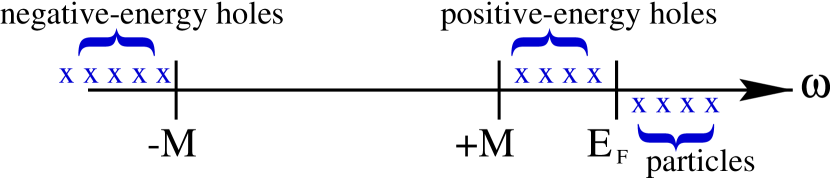
FIG. 1.: Spectral content of the nucleon propagator in a relativistic Fermi-gas approximation.

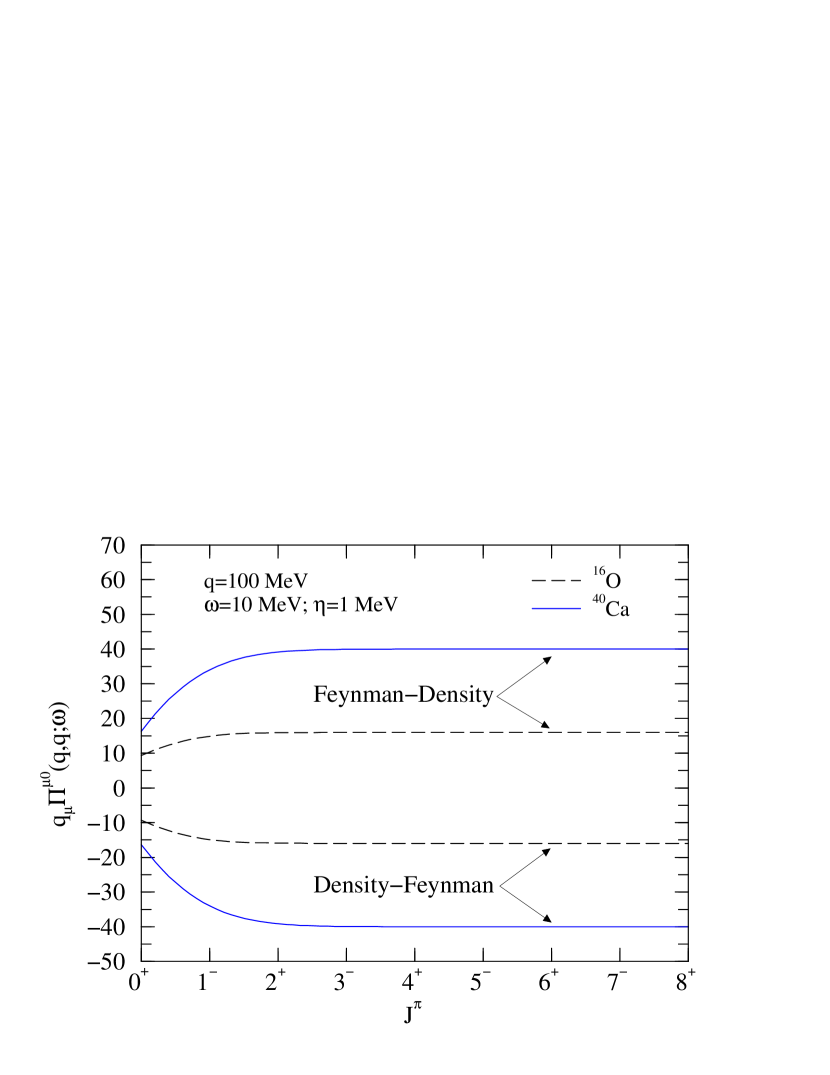
FIG. 2.: The real part of $q_{\mu}\Pi^{\mu 0}$ for the Feynman-Density and Density-Feynman parts of the nuclear polarization as a function of the total angular momentum channel. Results are reported for ¹⁶O and ⁴⁰Ca at $q\!=\!q^{\prime}\!=\!100$ MeV and $\omega\!=\!10$ MeV. In a consistent mean-field formalism these quantities should approach $\pm A$, respectively.

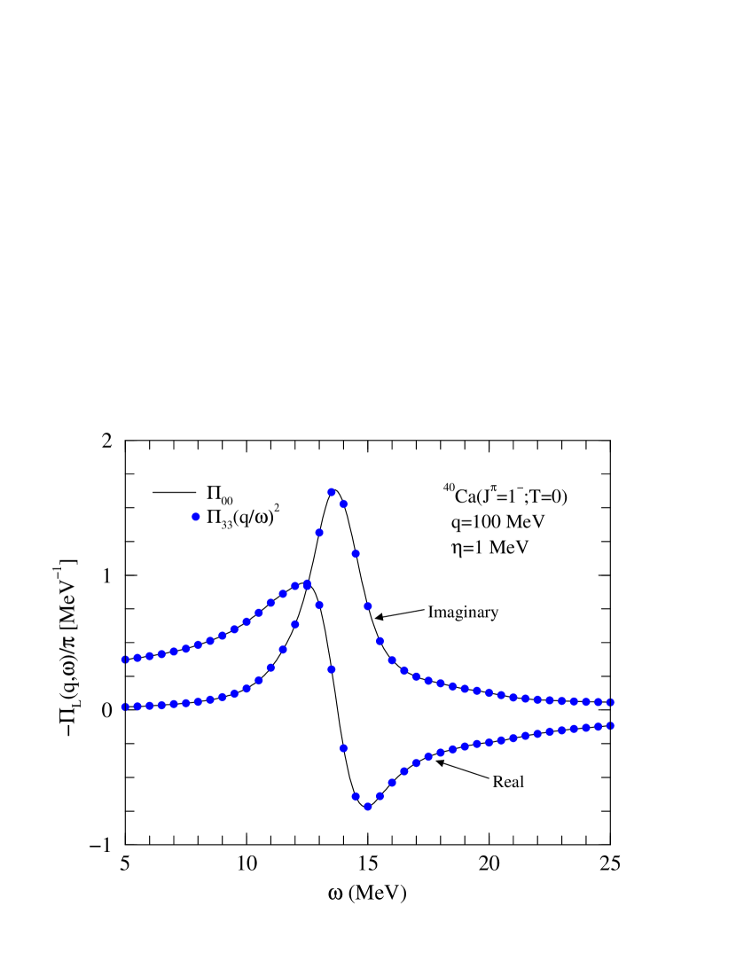
FIG. 3.: The longitudinal polarization for the isoscalar dipole state computed from the timelike component of the vector current (solid line) and from the longitudinal component (filled circles). In a consistent mean-field formalism — such as the one used here — they should be identical. Note that the imaginary component is the longitudinal response.

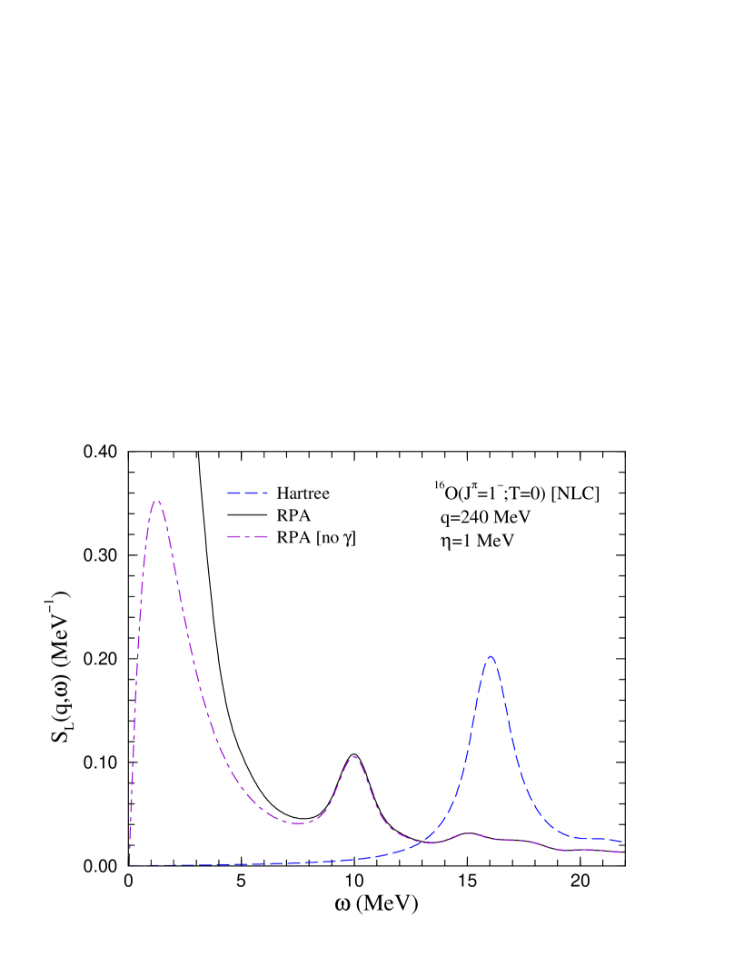
FIG. 4.: Isoscalar dipole strength in ¹⁶O in lowest-order Hartree (dashed line) and in a consistent RPA (solid line) approximation. The dot-dashed line is the RPA response with a residual interaction that lacks the contribution from the isoscalar component of the photon. The nonlinear model NLC was employed in the calculation.

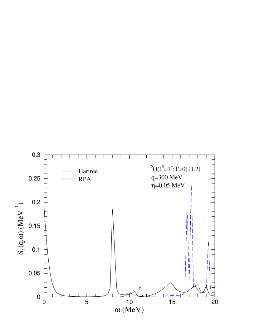
FIG. 5.: Distribution of isoscalar-dipole strength in ¹⁶O in a lowest-order Hartree (dashed line) and in a consistent RPA (solid line) approximation. The linear model L2 was employed in the calculation.

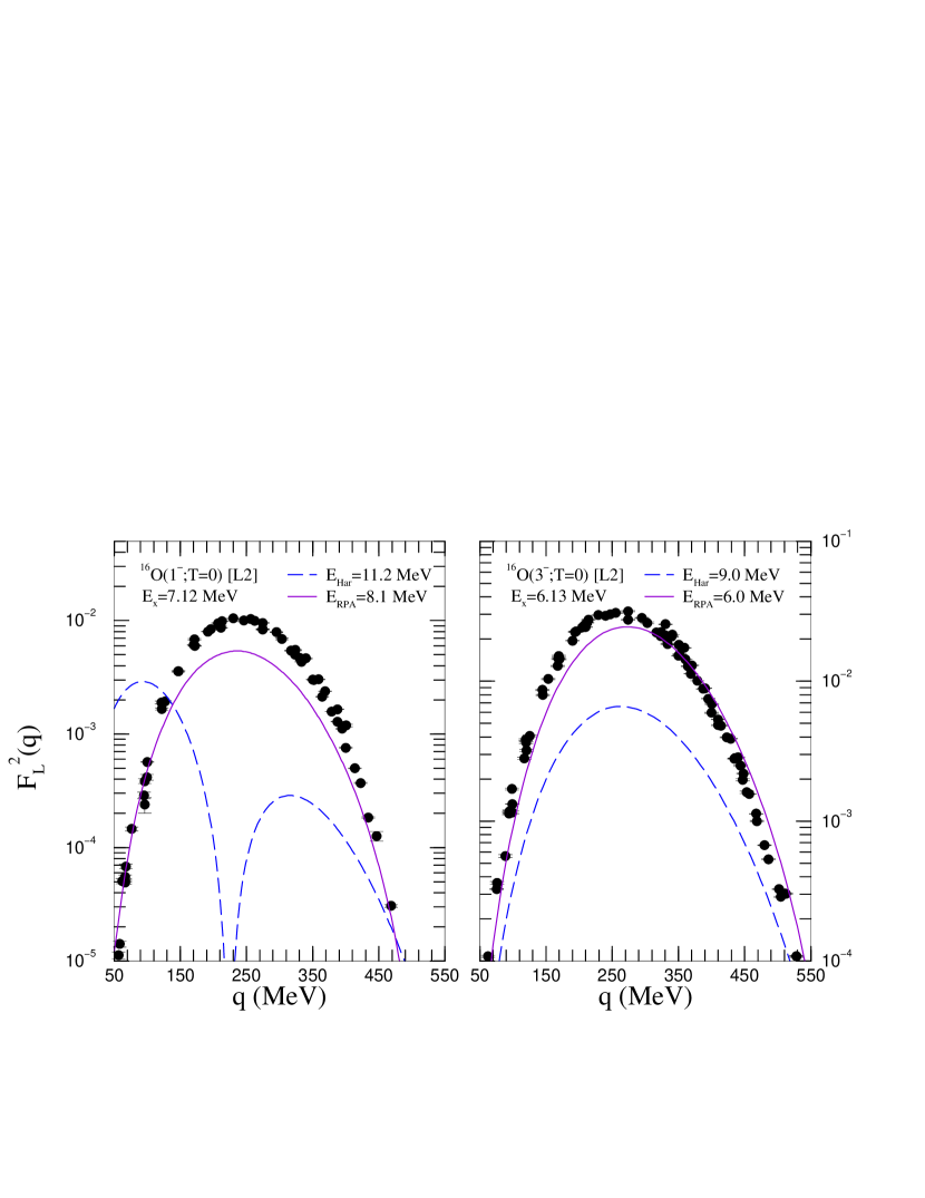
FIG. 6.: Inelastic isoscalar-dipole (left panel) and isoscalar-octupole (right panel) form-factors for ¹⁶O in a lowest-order Hartree (dashed line) and in a consistent RPA (solid line) approximation. The linear model was employed in the calculation and the experimental data is from Ref. [41].

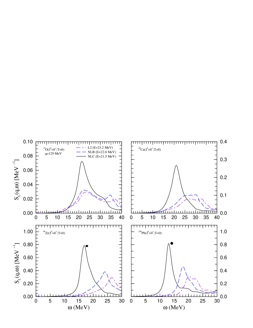
FIG. 7.: Nuclear dependence of the isoscalar giant monopole resonance in three relativistic mean-field models.

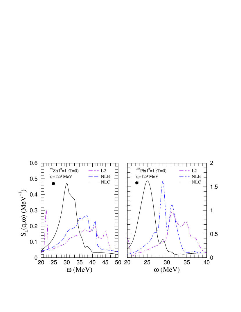
FIG. 8.: Nuclear dependence of the isoscalar giant dipole resonance in three relativistic mean-field models.

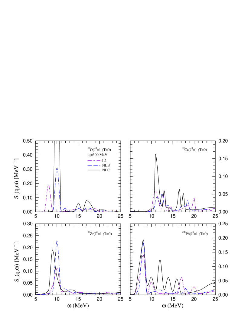
FIG. 9.: Low-energy component of the isoscalar dipole strength in three relativistic mean-field models.

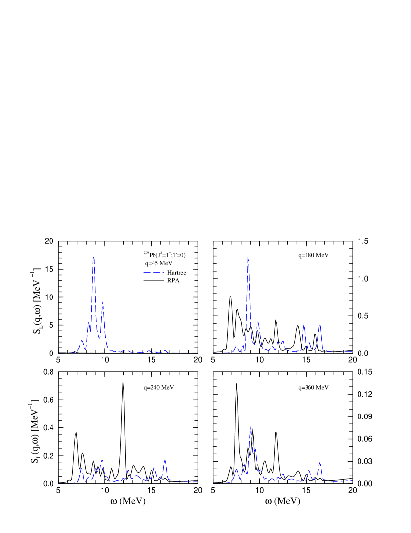
FIG. 10.: Momentum-transfer dependence of the low-energy component of the isoscalar dipole strength in a lowest-order Hartree (dashed line) and RPA (solid line) approximations. All calculations were performed using the NLC set.