$K_{l3}$ transition form factors

Abstract

The rainbow truncation of the quark Dyson–Schwinger equation is combined with the ladder Bethe–Salpeter equation for the meson bound state amplitudes and the dressed quark-W vertex in a manifestly covariant calculation of the $K_{l3}$ transition form factors and decay width in impulse approximation. With model gluon parameters previously fixed by the chiral condensate, the pion mass and decay constant, and the kaon mass, our results for the $K_{l3}$ form factors and the kaon semileptonic decay width are in good agreement with the experimental data.

Pacs Numbers: 24.85.+p, 14.40.Aq, 13.20.-v, 11.10.St

I Introduction

The central unknown quantity required for reliable calculations of weak decay amplitudes are the hadronic matrix elements. In this respect, the semileptonic $K_{l3}$ decay is an interesting process: pseudoscalar mesons are well-understood as Goldstone bosons, only the vector part of the weak interaction is involved, and there are experimental data available which allows one to judge various theoretical (model) calculations. These calculations generally fall into two different classes: effective theories using meson degrees of freedom, e.g. chiral perturbation theory [1, 2], and models employing quark and gluon degrees of freedom, e.g. constituent quark models [3, 4, 5] and the Dyson–Schwinger approach [6, 7, 8].

In particular, the light-front approach has been a popular framework for a Hamiltonian approach to analyze exclusive hadronic processes [9], and the pseudoscalar-to-pseudoscalar weak transition form factors have been studied within a light-front constituent quark model in Ref. [4, 5]. One complication of the light-front formalism is that in the analysis of timelike exclusive processes one needs to take into account light-front nonvalence contributions, which are absent in a manifestly Poincarè invariant approach. Recently, an effective treatment has been presented [10] to incorporate such contributions, and a systematic program has been laid out [11] to take into account the nonvalence contributions. However, the systematic program explicitly requires all higher Fock-state components while there has been relatively little progress in computing the basic wave-functions of hadrons from first principles. Furthermore, the (nonperturbative) dressing of the quark-W vertex and the dynamical chiral symmetry breaking are yet underdeveloped aspects in this approach. In particular the latter aspect needs to be seriously considered for processes involving pions and kaons, which are the pseudo-Goldstone bosons associated with dynamical chiral symmetry breaking [12, 13].

In this work we use the set of Dyson–Schwinger equations [DSEs] to calculate the $K_{l3}$ transition form factors. The DSEs provide us with a manifestly covariant approach which is consistent with dynamical chiral symmetry breaking [14], electromagnetic current conservation [15], and quark and gluon confinement [16]. For recent reviews on the DSE and its application to hadron physics, see Refs. [17, 18]. Our calculation of the $K_{l3}$ transition form factors is analogous to recent calculations of the pion and kaon electromagnetic form factors in impulse approximation [15]. Here we demonstrate that in the same framework, with a consistent dressing of the quark-W vertex, we can also describe the semileptonic decay of both the neutral and charged kaons, without any readjustment of the model parameters. In Sec. II we review the formulation that underlies a description of the meson form factors within a modeling of QCD through the DSEs, and discuss the details of the model. In Sec. III we present our numerical results for the form factors and decay widths. A discussion of our results is given in Sec. IV.

II Meson form factors within the DSE approach

The matrix elements describing kaon semileptonic decays are

$$J_{\mu}^{K^{+}}(P,Q) = \langle\pi^{0}(p)|\bar{s}\gamma_{\mu}u|K^{+}(k)\rangle$$ (1)

$$= \frac{1}{\sqrt{2}}\left(f_{+}(-Q^{2})P_{\mu}+f_{-}(-Q^{2})Q_{\mu}\right)\,,$$ (2)

for the charged kaon, and for the neutral kaon

$$J_{\mu}^{K^{0}}(P,Q) = \langle\pi^{-}(p)|\bar{s}\gamma_{\mu}u|K^{0}(k)\rangle$$ (3)

$$= f_{+}(-Q^{2})P_{\mu}+f_{-}(-Q^{2})Q_{\mu}\,,$$ (4)

where $P_{\mu}=(p+k)_{\mu}$ and $Q_{\mu}=(k-p)_{\mu}$, with $P\cdot Q=m_{\pi}^{2}-m_{k}^{2}$ for on-shell pions and kaons. Alternatively, we can decompose $J_{\mu}^{K^{0}}$ into its transverse and longitudinal components

$$J_{\mu}^{K^{0}}(P,Q) = f_{+}(-Q^{2})\;T_{\mu\nu}(Q)\,P_{\nu}+f_{0}(-Q^{2})\,\frac{P\cdot Q}{Q^{2}}\;Q_{\mu}\,,$$ (5)

with $T_{\mu\nu}$ the transverse projection operator

$$T_{\mu\nu}(Q) = \left(\delta_{\mu\nu}-\frac{Q_{\mu}Q_{\nu}}{Q^{2}}\right)\,.$$ (6)

In the isospin-symmetric limit, which we employ here, the form factors $f_{\pm}(t=-Q^{2})$ and $f_{0}(t)$ are the same for the $K^{+}$ and the $K^{0}$.

In impulse approximation, these matrix elements are given by

$$J_{\mu}^{K^{0}}(P,Q) = N_{c}\int\!\!\frac{d^{4}q}{(2\pi)^{4}}\,{\rm Tr}\big{[}S^{d}(q)\,\Gamma_{K}^{d\bar{s}}(q,q-k)S^{s}(q-k)\,i\Gamma^{s\bar{u}W}_{\mu}(q-k,q-p)\,S^{u}(q-p)\,\bar{\Gamma}_{\pi}^{u\bar{d}}(q-p,q)\big{]}\;,$$ (7)

where $S^{f}$ is the dressed quark propagator with flavor index $f$, $\Gamma_{\pi\,(K)}$ the pion (kaon) Bethe–Salpeter amplitude [BSA], and $\Gamma^{s\bar{u}W}_{\mu}$ the dressed $s\bar{u}W$ vertex, each satisfying their own DSE. Note that the coupling constant and the CKM matrix element $V_{us}$ are removed from the definition of the quark-W vertex.

A Dyson–Schwinger Equations

The DSE for the renormalized quark propagator in Euclidean space is

$$S(p)^{-1} = i\,Z_{2}\,/\!\!\!p+Z_{4}\,m(\mu)+Z_{1}\int^{\Lambda}\!\!\!\frac{d^{4}q}{(2\pi)^{4}}\,g^{2}D_{\mu\nu}(k)\frac{\lambda^{a}}{2}\gamma_{\mu}S(q)\Gamma^{a}_{\nu}(q,p)\,,$$ (8)

where $D_{\mu\nu}(k)$ is the dressed-gluon propagator, $\Gamma^{a}_{\nu}(q;p)$ the dressed-quark-gluon vertex, and $k=p-q$. The most general solution of Eq. (8) has the form $S(p)^{-1}=i/\!\!\!pA(p^{2})+B(p^{2})$ and is renormalized at spacelike $\mu^{2}$ according to $A(\mu^{2})=1$ and $B(\mu^{2})=m(\mu)$ with $m(\mu)$ the current quark mass. The notation $\int^{\Lambda}$ represents a translationally invariant regularization of the integral with $\Lambda$ the regularization mass-scale; at the end of all calculations this regularization scale can be removed.

Mesons can be studied by solving the homogeneous Bethe–Salpeter equation [BSE] for $q^{a}\bar{q}^{b}$ bound states, with $a$ and $b$ flavor indices,

$$\Gamma^{a\bar{b}}_{H}(p_{+},p_{-}) = \int^{\Lambda}\!\!\!\frac{d^{4}q}{(2\pi)^{4}}\,K(p,q;Q)\otimes S^{a}(q_{+})\,\Gamma^{a\bar{b}}_{H}(q_{+},q_{-})\,S^{b}(q_{-})\,,$$ (9)

where $p_{+}=p+\eta Q$ and $p_{-}=p-(1-\eta)Q$ are the outgoing and incoming quark momenta respectively, and similarly for $q_{\pm}$. The kernel $K$ is the renormalized, amputated $q\bar{q}$ scattering kernel that is irreducible with respect to a pair of $q\bar{q}$ lines. This equation has solutions at discrete values of $Q^{2}=-m_{H}^{2}$, where $m_{H}$ is the meson mass. Together with the canonical normalization condition for $q\bar{q}$ bound states, it completely determines $\Gamma_{H}$, the bound state BSA. The different types of mesons, such as (pseudo-)scalar, (axial-)vector, and tensor mesons, are characterized by different Dirac structures. The most general decomposition for pseudoscalar bound states is [13]

$$\Gamma_{PS}(k_{+},k_{-}) = \gamma_{5}\big{[}iE(k^{2};k\cdot Q;\eta)+\;/\!\!\!\!Q\,F(k^{2};k\cdot Q;\eta)+\,/\!\!\!k\,G(k^{2};k\cdot Q;\eta)+\sigma_{\mu\nu}\,Q_{\mu}k_{\nu}\,H(k^{2};k\cdot Q;\eta)\big{]}\,,$$ (10)

where the invariant amplitudes $E$, $F$, $G$ and $H$ are Lorentz scalar functions of $k^{2}$ and $k\cdot Q$. Note that these amplitudes explicitly depend on the momentum partitioning parameter $\eta$. However, so long as Poincaré invariance is respected, the resulting physical observables are independent of this parameter [15].

In order to describe weak (and electromagnetic) form factors one also needs the dressed $q\bar{q}W$ (and $q\bar{q}\gamma$) vertices. These vertices satisfy an inhomogeneous BSE: e.g. the $s\bar{u}W$ vertex $\Gamma^{u\bar{s}W}_{\mu}(p_{+},p_{-})$ satisfies

$$\Gamma^{s\bar{u}W}_{\mu}(p_{+},p_{-}) = Z_{2}\,(\gamma_{\mu}-\gamma_{\mu}\gamma_{5})+\int^{\Lambda}\!\!\!\frac{d^{4}q}{(2\pi)^{4}}\,K(p,q;Q)\otimes S^{s}(q_{+})\,\Gamma^{s\bar{u}W}_{\mu}(q_{+},q_{-})\,S^{s}(q_{-})\,.$$ (11)

B Model Truncation

To solve the BSE, we use a ladder truncation, with an effective quark-antiquark interaction that reduces to the perturbative running coupling at large momenta [13, 19]

$$K(p,q;P)\to-{\cal G}(k^{2})\,D_{\mu\nu}^{\rm free}(k)\textstyle{\frac{\lambda^{i}}{2}}\gamma_{\mu}\otimes\textstyle{\frac{\lambda^{i}}{2}}\gamma_{\nu}\,,$$ (12)

where $D_{\mu\nu}^{\rm free}(k=p-q)$ is the free gluon propagator in Landau gauge. The corresponding rainbow truncation of the quark DSE, Eq. (8), is given by $\Gamma^{i}_{\nu}(q,p)\rightarrow\gamma_{\nu}\lambda^{i}/2$ together with $Z_{1}g^{2}D_{\mu\nu}(k)\rightarrow{\cal G}(k^{2})D_{\mu\nu}^{\rm free}(k)$. This combination of rainbow and ladder truncation preserves both the vector and axial-vector Ward–Takahashi identities. This ensures that pions are (almost) massless Goldstone bosons associated with dynamical chiral symmetry breaking [13]; in combination with impulse approximation for meson form factors, Eq. (7), it also ensures current conservation. Furthermore, this truncation was found to be particularly suitable for the flavor octet pseudoscalar and vector mesons since the next-order contributions in a quark-gluon skeleton graph expansion, have a significant amount of cancellation between repulsive and attractive corrections [20].

The model is completely specified once a form is chosen for the “effective coupling” ${\cal G}(k^{2})$. We employ the Ansatz [19]

$$\frac{{\cal G}(k^{2})}{k^{2}} = \frac{4\pi^{2}\,D\,k^{2}}{\omega^{6}}\,{\rm e}^{-k^{2}/\omega^{2}}+\frac{4\pi^{2}\,\gamma_{m}\;{\cal F}(k^{2})}{\textstyle{\frac{1}{2}}\ln\left[\tau+\left(1+k^{2}/\Lambda_{\rm QCD}^{2}\right)^{2}\right]}\;,$$ (13)

with $\gamma_{m}=12/(33-2N_{f})$ and ${\cal F}(s)=(1-\exp\frac{-s}{4m_{t}^{2}})/s$. The ultraviolet behavior is chosen to be that of the QCD running coupling $\alpha(k^{2})$; the ladder-rainbow truncation then generates the correct perturbative QCD structure of the DSE-BSE system of equations. The first term implements the strong infrared enhancement in the region $0<k^{2}<1\,{\rm GeV}^{2}$ phenomenologically required [21] to produce a realistic value for the chiral condensate. We use $m_{t}=0.5\,{\rm GeV}$, $\tau={\rm e}^{2}-1$, $N_{f}=4$, $\Lambda_{\rm QCD}=0.234\,{\rm GeV}$, and a renormalization scale $\mu=19\,{\rm GeV}$ which is well into the perturbative domain [13, 19]. The remaining parameters, $\omega=0.4\,{\rm GeV}$ and $D=0.93\,{\rm GeV}^{2}$ along with the quark masses, are fitted to give a good description of the chiral condensate, $m_{\pi/K}$ and $f_{\pi}$.

Within this model, the quark propagator reduces to the perturbative propagator in the ultraviolet region. However, in the infrared region both the wave function renormalization $Z(p^{2})=1/A(p^{2})$ and the dynamical mass function $M(p^{2})=B(p^{2})/A(p^{2})$ deviate significantly from the perturbative behavior, due to chiral symmetry breaking. It is interesting to note that the typical results obtained using the rainbow DSE, a significant enhancement of $M(p^{2})$ below $1\;{\rm GeV}^{2}$ and also an enhancement of $A(p^{2})$, have recently been confirmed by lattice simulations [22]; with the present ladder DSE model, the functions $Z$ and $M$ are in semiquantitative agreement with the forms obtained in lattice simulations [23].

The vector meson masses and electroweak decay constants one obtains in this model are in good agreement with experiments [19]. Without any readjustment of the parameters, one gets remarkable agreement with the most recent Jlab data for $F_{\pi}$ [24], and also for other electromagnetic charge radii and form factors [15, 25]. The strong decays of the vector mesons into a pair of pseudoscalar mesons are also well-described within this model [26]. Here we apply the same approach to the kaon semileptonic decay.

III Numerical results

To calculate the form factors $f_{\pm}(t)$, we start by solving the quark DSE in rainbow approximation, and subsequently use its solution to solve the homogeneous BSE, Eq. (9), for the pseudoscalar bound states, and the inhomogeneous BSE, Eq. (11), for the quark-W vertex, using the ladder truncation, Eq. (12). With these BS amplitudes and quark propagators, we then calculate the form factors in impulse approximation using Eq. (7). In the SU(3) flavor limit, $f_{+}=F_{\pi}$, the pion electromagnetic form factor, and $f_{-}=0$. We therefore expect $f_{+}$ to be of order one for small $t$. On the other hand, $f_{-}$, which is a measure of the constituent mass ratio $M_{s}/M_{u}$ [3], is expected to be significantly smaller. This expectation is indeed confirmed by our calculations, see Fig. 1.

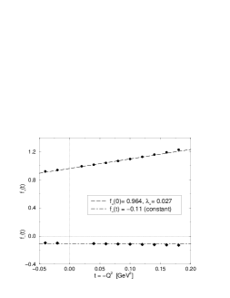
FIG. 1.: Our results for $f_{+}(t)$ (solid dots) with linear fit (dashed line), and $f_{-}(t)$ (solid diamonds) with a constant fit (dot-dashed line) in the physical region.

In the physical region, $m_{l}^{2}<t<(m_{K}-m_{\pi})^{2}\simeq 0.13\;{\rm GeV}^{2}$, our results for $f_{\pm}(t)$ are almost linear. The experimental data are often analyzed in terms of $f_{+}$ and $f_{0}$, using a linear parametrisation

$$f(t) = f(0)\Big{(}1+\frac{\lambda}{m_{\pi}^{2}}\;t\,\Big{)}\,.$$ (14)

Such a linear parametrisation for both $f_{+}$ and $f_{0}$ implies that $f_{-}$ is independent of $t$, since $f_{0}$ is related to $f_{\pm}$ via

$$f_{0}(t) = f_{+}(t)+\frac{t}{m_{K}^{2}-m_{\pi}^{2}}f_{-}(t)\,.$$ (15)

To within a few percent, $f_{-}$ is indeed almost constant in the physical region, $0<t<0.13~{}{\rm GeV}^{2}$, as can be seen from Fig. 1. Our results are summarized in Table I, where we have included a slope parameter $\lambda$ for $f_{-}(t)$ as well.

Our results agree quite well with the available data for $f_{+}(t)$, see Fig. 2. Also the results for other observables compare reasonably well with the experimental data, given the error bars, and the differences between the form factor parameters extracted from the charged and the neutral kaon decay, see Table I. The partial decay width for $K\rightarrow\pi\,e\nu_{e}$ and $K\rightarrow\pi\,\mu\nu_{\mu}$ is obtained by integrating the decay rate

$$\frac{d\Gamma}{dt} = \frac{G_{F}\,|V_{us}|^{2}}{24\pi^{3}}\left(1-\frac{m_{l}^{2}}{t}\right)^{2}K(t)\Bigg{[}K^{2}(t)\,\left(1+\frac{m_{l}^{2}}{2\,t}\right)\;|f_{+}(t)|^{2}+m_{K}^{2}\,\left(1-\frac{m_{\pi}^{2}}{m_{K}^{2}}\right)^{2}\,\frac{3\,m_{l}^{2}}{8\,t}\;|f_{0}(t)|^{2}\Bigg{]}\;,$$ (16)

where

$$K(t) = \frac{1}{2m_{K}}\left((m_{K}^{2}+m_{\pi}^{2}-t)^{2}-4m_{K}^{2}m_{\pi}^{2}\right)^{\frac{1}{2}}\,,$$ (17)

and $m_{l}$ is the lepton mass. Again, we find good agreement with the data, see Table I.

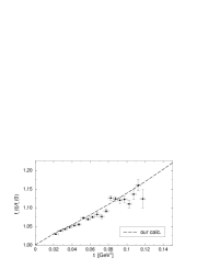
FIG. 2.: Our results for $f_{+}(t)$, normalized to $f_{+}(0)=1$, compared to the experimental results [27].

For comparison, we have also included the results from some other model calculations [7, 10] and from 1-loop chiral perturbation theory [2, 29]. Our results compare quite well with chiral perturbation theory, not only for the slope parameters, but also for the curvature of the form factors. A prediction from current algebra is the value of $f_{0}(t)$ at the Callan–Treiman point, $t=m^{2}_{K}-m^{2}_{\pi}$, namely $f_{K}/f_{\pi}=1.22~{}$[2, 30]. The reason we get $f_{0}(m^{2}_{K}-m^{2}_{\pi})=1.18$ instead of $1.22$ is related to our value of $f_{K}$: we obtain $f_{K}=109~{}{\rm MeV}$ in our model [13, 19], compared to the experimental value $113~{}{\rm MeV}$. Because our approach satisfies constraints coming from current conservation and the axial-vector Ward–Takahashi identity, it is not surprising that we indeed agree with these predictions from chiral perturbation theory.

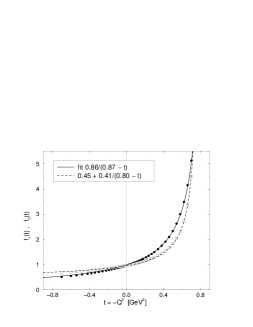
FIG. 3.: Our results for $f_{+}(t)$ (solid dots) with monopole fit (solid curve), and $f_{0}(t)$ (open squares) with a constant plus monopole fit(dashed curve).

Outside the physical region, $f_{\pm}(t)$ and $f_{0}(t)$ are clearly not linear, as shown in Fig. 3. In the region we considered, our result for $f_{+}(t)$ is very well approximated by a monopole, with monopole mass $m^{2}=0.87\;{\rm GeV}^{2}$. The reason for this monopole behavior is easy to understand: the vertex function $\Gamma^{s\bar{u}W}_{\mu}$ has a resonance peak in its transverse vector components at the $K^{*}$ mass, because the homogeneous version of Eq. (11) has a solution at $Q^{2}=-m_{K^{*}}^{2}$, corresponding to the $K^{*}$ vector meson. The longitudinal part of the quark-W vertex has a resonance peak at the location of the $u\bar{s}$ scalar bound state. We tentatively identify this with the $K_{0}^{*}(1430)$ meson; however, in contrast to vector states, the use of ladder approximation is expected to be inadequate for scalars [31]. Near these bound states, the vertex behaves like

$$\Gamma^{s\bar{u}W}_{\mu}(p_{+},p_{-};Q) \sim \Gamma_{\mu}^{\hbox{regular}}(p_{+},p_{-};Q)+\frac{r_{V}\;T_{\mu\nu}(Q)}{Q^{2}+m_{K^{*}}^{2}}\Gamma^{K^{*}}_{\nu}(p_{+},p_{-};Q)+\frac{r_{S}\;Q_{\mu}}{Q^{2}+m_{K_{0}^{*}}^{2}}\Gamma^{K_{0}^{*}}(p_{+},p_{-};Q)\,,$$ (18)

where $\Gamma^{K^{*}}$ and $\Gamma^{K_{0}^{*}}$ are the bound state BSAs, and $r_{V}$ and $r_{S}$ the residues of the vertex at these poles [12]. In our model we have actual poles in the quark-W vertex, rather than resonance peaks, because we have not included meson loop corrections in our kernel, and therefore we do not generate a width for the $K^{*}$ nor the $K^{*}_{0}$. In the spacelike region and at small timelike $t=-Q^{2}$ we expect these corrections to be small. However, they will modify our results significantly close to the resonance peak.

As can be seen from Eq. (7), these poles in $\Gamma^{s\bar{u}W}_{\mu}$ lead a similar behavior of $J^{K^{0}}_{\mu}$ near these poles. From Eq. (5) it is clear that the vector meson pole leads to a pole in $f_{+}(t)$, but not in $f_{0}(t)$, whereas the scalar meson induces a pole in $f_{0}(t)$ but not in $f_{+}(t)$

$$f_{0}(-Q^{2}) = \frac{-Q_{\mu}\;J^{K^{0}}_{\mu}}{m_{K}^{2}-m_{\pi}^{2}}\;,$$ (19)

$$f_{+}(-Q^{2}) = \frac{\left(Q^{2}P_{\mu}+(m_{K}^{2}-m_{\pi}^{2})\,Q_{\mu}\right)\,J^{K^{0}}_{\mu}}{Q^{2}\,P^{2}-(m_{K}^{2}-m_{\pi}^{2})^{2}}\;.$$ (20)

Note that $f_{-}(t)$ will in general be sensitive to both the scalar and the vector meson bound state.

The present model has a vector bound state at $t=0.876\;{\rm GeV}^{2}$ (cf. the experimental mass $m_{K^{*}}^{2}=0.796\;{\rm GeV}^{2}$) [19]. Thus the monopole behavior of the form factor $f_{+}(t)$ in Fig. 3 simply reflects the existence of this pole. A similar behavior was found in the pion and kaon electromagnetic form factors [15]. The physical $f_{+}(t)$ can be expected to rise more slowly with $t$ than our present calculations due to meson loop corrections, and will develop a nonzero imaginary part above the threshold for intermediate $\pi\,K$ states.

The scalar form factor $f_{0}(t)$ does also exhibit the expected pole behavior, and we are able to identify the scalar and the vector poles separately, see Fig. 3. The lowest $u\bar{s}$ scalar bound state in this model has a mass of $m^{2}=0.80\;{\rm GeV}^{2}$, which is rather low compared to the $K^{*}_{0}(1430)$ with a mass $m^{2}=2.04\;{\rm GeV}^{2}$; on the other hand, it could be an indication that there exists a light scalar resonance $\kappa(900)$, as has been speculated [32]. Something similar happens in in the $u/d$ quark sector: in rainbow-ladder truncation, one typically finds a scalar $u/d$ bound state around $m=0.6$ to $0.7\;{\rm GeV}$ [33, 34, 35], just below the $\rho$ mass. This bound state could either correspond to a broad $\sigma$, or to the $f_{0}$ and/or $a_{0}$, in which case the calculated mass is about 30 to 40% too low. It is known that the leading perturbative corrections to the ladder kernel cancel to a large extent in both the pseudoscalar and vector channel, but not in the scalar channel; we therefore expect in the scalar channel significant repulsive corrections to the ladder kernel which could increase the mass of the scalar bound state [31]. We also expect meson loop corrections to be more important in the scalar channel than in the vector channel. Therefore, our calculation for $f_{0}(t)$ should not be trusted quantitatively in the timelike region beyond the Callan–Treiman point, $t=0.23~{}{\rm GeV}^{2}$.

In the spacelike asymptotic region $f_{+}$ and $f_{0}$ seem to behave differently: a monopole fit does not work for $f_{0}$. In order to fit $f_{0}$, we either need to add a nonzero constant, or use at least two monopoles. Simple power counting indicates that $J_{\mu}^{K^{0}}$ scales like $1/Q$; inserting this behavior in Eqs. (19) and (20) implies that $f_{+}(t)$ falls like $1/t$, but $f_{0}(t)$ goes to a constant (up to logarithmic corrections) at large spacelike $t$ (remember that $P$ scales like $Q$ in the asymptotic region). This behavior of $f_{+}$ agrees with the pQCD predictions for the electromagnetic pion and kaon form factor [36]; the behavior of $f_{0}$ can be understood if one realizes that the combination $f_{0}(t)\,\frac{m^{2}_{K}-m^{2}_{\pi}}{t}$ does fall like $1/t$ if $f_{0}(t)$ goes to a constant.

IV Discussion

Using the rainbow-ladder truncation of the set of DSEs with a model for the effective quark-antiquark interaction that has been fitted to the chiral condensate and $f_{\pi}$, we study the $K_{l3}$ decay in impulse approximation. Our results, both for the form factors and for the decay width, are in good agreement with experimental data, without any readjustment of the parameters; they also compare quite well with chiral perturbation theory. Note however that in chiral perturbation theory the pion charge radius is used as input, in order to fix a low-energy constant, which is important for these form factors as well, in particular for $\lambda_{+}$. In our calculation, the only model parameters are in the infrared behavior of the effective quark-antiquark interaction, which were fitted to the chiral condensate and the pion decay constant [19]; the pion charge radius follows from a calculation similar to the one presented here for the $K_{l3}$ decay [15].

Our approach is based on previous work by Kalinovsky et al. [7], and the results are quite similar. However, an important difference with this earlier study is that we dress the quark-W vertex by solving the inhomogeneous BSE for this vertex. The main advantage of doing so is that we thus automatically include effects coming from intermediate vector and scalar mesons. Another difference is that here we use actual solutions of a DSE for the propagators and BS amplitudes in Eq. (7), rather than phenomenological parametrisations, which reduces the number of parameters in the calculation.

We have demonstrated explicitly that both $f_{+}(t)$ and $f_{0}(t)$ exhibit resonance peaks in the timelike region due to the existence of vector and scalar bound states respectively. The effects of meson loops are not included in our present calculation, which is why we find a pole behavior rather than a resonance peak. In Ref. [7] it was already demonstrated that non-analytic effects from such loops could contribute significantly to the behavior of the form factors, not only beyond the threshold for $\pi K$ production, but also in the physical region. We hope to be able to incorporate these effects in future work.

Our results are also similar to those obtained recently by Ji and Choi [10] in a light-front calculation, at least for $f_{+}(t)$, which dominates this decay, even though details of the calculation are quite different. In light-front calculations of timelike processes one has to include particle-number-nonconserving Fock states to recover the Lorentz covariance, which complicates the calculation [10, 11]. Since our approach is manifestly covariant, such contributions are automatically included in our impulse approximation. Another difference is that we use momentum-dependent quark self-energies, consistent with dynamical chiral symmetry breaking, whereas in Ref. [10] constituent quarks with fixed masses are used. Recently, the effects of a running quark mass (instead of a fixed constituent mass) have been explored in a light-front calculation of the pion form factor [37]. It would be interesting to see the effect of such a running mass on the $K_{l3}$ form factors, in particular on $f_{-}(t)$, which in general appears to be quite sensitive to details of the calculation.

	our	experiment		other theory
	calc	$K^{+}$	$K^{0}$	$\chi$PT [2, 29]	DSE model [7]	light cone [10]
$f_{+}(0)$	0.964			0.977	0.98	0.962
$\lambda_{+}(e3)$	0.027	$.0276\pm.0021$	$.0288\pm.0015$	0.031	0.028	0.026
$\lambda_{+}(\mu 3)$	0.027	$.031\pm.008$	$.034\pm.005$	0.031	0.029	0.026
$-f_{-}(0)$	0.10			0.16	0.24
$\lambda_{-}$	0.03				0.023
$-\xi=-f_{-}(0)/f_{+}(0)$	0.11	$0.31\pm.15$	$0.11\pm.09$	0.17	0.25	0.01
$\lambda_{0}$	0.018	$.006\pm.007$	$.025\pm.006$	0.017	0.007	0.025
$f_{0}(m^{2}_{K}-m^{2}_{\pi})$	1.18			1.22	1.18
$\Gamma(K_{e3})$	7.38	3.89	7.50			7.3
$\Gamma(K_{\mu 3})$	4.90	2.57	5.26			4.92

TABLE I.: Our results, compared to data [28] where available and some other calculations. The partial decay width is in $10^{6}\;{\rm s}^{-1}$; because $J_{\mu}^{K^{+}}=J_{\mu}^{K^{0}}/\sqrt{2}$ in the exact isospin limit, the experimental value for the $K^{+}$ partial decay width should be multiplied by a factor of two, in order to compare it with our calculation and with the $K^{0}$ partial decay width.

REFERENCES

- [1] H. Leutwyler and M. Roos, Z. Phys. C25, 91 (1984).
- [2] J. Gasser and H. Leutwyler, Nucl. Phys. B250, 517 (1985).
- [3] N. Isgur, Phys. Rev. D 12, 3666 (1975).
- [4] H. Choi and C. Ji, Phys. Rev. D 59, 034001 (1999) [hep-ph/9807500].
- [5] H. Choi and C. Ji, Phys. Lett. B460, 461 (1999) [hep-ph/9903496].
- [6] A. Afanasev and W. W. Buck, Phys. Rev. D 55, 4380 (1997) [hep-ph/9606296].
- [7] Y. Kalinovsky, K. L. Mitchell and C. D. Roberts, Phys. Lett. B399, 22 (1997) [nucl-th/9610047].
- [8] M. A. Ivanov, Y. L. Kalinovsky and C. D. Roberts, Phys. Rev. D60, 034018 (1999) [nucl-th/9812063].
- [9] S. J. Brodsky, H. Pauli and S. S. Pinsky, Phys. Rept. 301, 299 (1998) [hep-ph/9705477].
- [10] C. Ji and H. Choi, hep-ph/0009281.
- [11] S. J. Brodsky and D. S. Hwang, Nucl. Phys. B543, 239 (1999) [hep-ph/9806358].
- [12] P. Maris, C. D. Roberts and P. C. Tandy, Phys. Lett. B420, 267 (1998) [nucl-th/9707003].
- [13] P. Maris and C. D. Roberts, Phys. Rev. C56, 3369 (1997) [nucl-th/9708029].
- [14] see e.g. K. Higashijima, Phys. Rev. D 29, 1228 (1984); V.A. Miransky, Phys. Lett. B 165, 401 (1985); D. Atkinson and P.W. Johnson, Phys. Rev. D 37, 2290 and 2296 (1988); C.D. Roberts and B.H. McKellar, Phys. Rev. D 41, 672 (1990).
- [15] P. Maris and P. C. Tandy, Phys. Rev. C61, 045202 (2000) [nucl-th/9910033]; ibid, Phys. Rev. C62, 055204 (2000) [nucl-th/0005015].
- [16] C.J. Burden, C.D. Roberts, and A.G. Williams, Phys. Lett. B 285, 347 (1992); G. Krein, C.D. Roberts, and A.G. Williams, Int. J. Mod. Phys. A 7, 5607 (1992); P. Maris, Phys. Rev. D 52, 6087 (1995).
- [17] C. D. Roberts and S. M. Schmidt, Prog. Part. Nucl. Phys. 45S1, 1 (2000) [nucl-th/0005064].
- [18] R. Alkofer and L. von Smekal, hep-ph/0007355.
- [19] P. Maris and P. C. Tandy, Phys. Rev. C60, 055214 (1999) [nucl-th/9905056].
- [20] A. Bender, C. D. Roberts and L. von Smekal, Phys. Lett. B380, 7 (1996) [nucl-th/9602012].
- [21] F. T. Hawes, P. Maris and C. D. Roberts, Phys. Lett. B440, 353 (1998).
- [22] J. I. Skullerud and A. G. Williams, hep-lat/0007028.
- [23] P. Maris, nucl-th/0009064.
- [24] J. Volmer et al. [The Jefferson Lab F(pi) Collaboration], nucl-ex/0010009.
- [25] P. Maris, nucl-th/0008048.
- [26] D. Jarecke, P. Maris, and P.C. Tandy, in preparation.
- [27] A. Apostolakis et al., Phys. Lett. B473, 186 (2000).
- [28] Particle Data Group, C. Caso et al., Eur. Phys. J. C3, 1 (1998).
- [29] J. Bijnens, G. Colangelo, G. Ecker and J. Gasser, hep-ph/9411311.
- [30] C.G. Callan and S.B. Treiman, Phys. Rev. Lett. 16, 153 (1966).
- [31] A. Bender, C. D. Roberts and L. Von Smekal, Phys. Lett. B 380, 7 (1996) [nucl-th/9602012]; C. D. Roberts, in Quark Confinement and the Hadron Spectrum II, edited by N. Brambilla and G.M. Propseri (World Scientific, Singapore, 1997), pp. 224-230 [nucl-th/9609039].
- [32] D. Black, A. H. Fariborz and J. Schechter, hep-ph/0008246; J. A. Oller and E. Oset, Phys. Rev. D 60, 074023 (1999) [hep-ph/9809337].
- [33] P. Jain and H. J. Munczek, Phys. Rev. D 48, 5403 (1993) [hep-ph/9307221].
- [34] C. J. Burden, L. Qian, C. D. Roberts, P. C. Tandy and M. J. Thomson, Phys. Rev. C 55, 2649 (1997) [nucl-th/9605027].
- [35] P. Maris, C. D. Roberts, S. M. Schmidt and P. C. Tandy, Phys. Rev. C 63, 025202 (2001) [nucl-th/0001064].
- [36] G. P. Lepage and S. J. Brodsky, Phys. Lett. B 87, 359 (1979).
- [37] L. S. Kisslinger, H. Choi and C. Ji, hep-ph/0101053.