DAPNIA/SPHN-01-02 JLAB-THY-01-6

The deuteron: structure and form factors

M. Garçon^a and J.W. Van Orden^b

1 A historical introduction

Diplon, deuton, deuteron: under different names, the nucleus of deuterium, or diplogen, has been the subject of intense studies since its discovery in 1932. As the only two-nucleon bound state, its properties have continuously been viewed as important in nuclear theory as the hydrogen atom is in atomic theory. Yet, ambiguities remain in the relativistic description of this system and the two-nucleon picture is incomplete: meson exchange and nucleon excitation into resonances should be considered in the deuteron description. The question of rare configurations where the two nucleons overlap and loose their identity is still under debate. We are still looking for the elusive effects of quarks in the nuclear structure.

In this year of the millenium, the present article will first attempt to recall the early discoveries, measurements and theories. It will then boldly jump over decades of continuous efforts, building upon these, to present not an exhaustive review but an up-to-date status of our understanding of the deuteron, with a special emphasis on its electromagnetic form factors. To do justice to some seventy years of activity in this field is an immense task which is more easily approached by quoting here several reviews along this path [1, 2, 3, 4, 5, 6, 7, 8, 9, 10, 11, 12, 13]. The important subject of electro- and photo-disintegration of the deuteron will be only partly covered, referring the reader to [14].

1.1 Discovery of the deuteron

The existence of the first isotope of hydrogen was suggested in 1931 by Birge and Menzel [15] in order to remove discrepancies between two different measurements of the atomic mass of hydrogen. A first estimate of an abundance ratio ¹H/²H = 4500 was inferred from this hypothesis, close indeed to the actual value of 6700. The stable isotope was discovered by Urey and collaborators [16] a few months later, investigating distilled samples of natural hydrogen for the optical atomic spectrum of ²H in a discharge tube. Isotopic separation to study the properties of deuterium quickly became an intense activity. Its mass was measured by Bainbridge [17]. While Chadwick was discovering the neutron, several tens of papers were written, in one years time, devoted to the study of deuterium. An illuminating summary of this early research was made by Bleakney and Gould [18]. In 1933, “deutons” were used as accelerated projectiles first at Berkeley [19], then at Caltech and at Cavendish. Chadwick and Goldhaber [20] measured the first photodisintegrations $\gamma d\rightarrow pn$ in 1934.

1.2 Early theories

In 1932, there was no satisfactory theory of the nucleus. The nucleus was thought to be composed of protons and electrons since these were the only known charged particles and nuclei were seen to emit electrons ($\beta$ decay). The electrons were needed to cancel the positive charge of some of the protons in order to account for nuclei with identical charges, but with different masses, and to allow for the possibility of binding of the nucleus by means of electric forces. This was clearly unsatisfactory because the Coulomb force could not account for the binding energies of nuclei and the attempt to construct the nuclei from the incorrect number of spin-1/2 particles could not produce the correct nuclear spins.

The discovery of the neutron, shortly after that of the deuteron, did not immediately eliminate the confusion since the previous model persisted by simply describing the neutron as a bound system of a proton and an electron. Based on this faulty assumption, Heisenberg produced the first model of proton-neutron force [21]. Since it was not possible to actually construct a description of the neutron with the $ep$ model, Heisenberg simply assumed that the $pn$ force could be described by a phenomenological potential and that the neutron was a spin-1/2 object like the proton. Based on an analogy with the binding of the H${}^{+}_{2}$ ion by electron sharing, Heisenberg proposed that the force must involve the exchange of both spin and charge in the form of $\sigma^{(1)}\cdot\sigma^{(2)}\tau^{(1)}\cdot\tau^{(2)}$. Forces containing the remaining forms of spin and isospin operators were soon introduced by Wigner [22], Majorana [23] and Bartlett [24]. In all cases the spatial form of the potentials was to be determined phenomenologically to reproduce the deuteron properties and the available nucleon-nucleon ($NN$) scattering data. In 1935Bethe and Peierls [25] wrote the Hamiltonian of the “diplon” with an explicit introduction of a short range interaction. This approach became the mainstay of nuclear physics which has produced considerable success in describing nuclear systems and reactions. The $ep$ model of the neutron was not completely abandoned until after the Fermi theory [26] of $\beta$ decay became widely accepted.

The progress in discoveries and understanding was then so great that, in spite of an otherwise bleak social or political situation in many countries involved, this period is recalled as “The Happy Thirties” from a physicist’s point of view [27].

One of the other great theoretical preoccupations of the late 1920’s and the 1930’s was the development of quantum field theory starting with the first works of Dirac on quantum electrodynamics (QED) [28], the Dirac equation for the electron [29] and the Dirac hole theory [30] with field theory reaching its final modern form with Heisenberg [31]. QED at this time was very successful at tree-level but the calculation of finite results from loops was not really tractable until the introduction of systematic renormalization schemes in the late 1940’s. The first attempt to apply quantum field theory to the strong nuclear force was Yukawa’s suggestion [32] that the force was mediated by a new strongly coupling massive particle which became known as the pion. This started another strong thread in the theoretical approach of the nucleus by using meson-nucleon theory to obtain nuclear forces consistent with the phenomenological potential approach. The primary attraction of this approach is that a more microscopic description of the degrees of freedom of the problem is provided and that additional constraints are imposed on the theory by the necessity of simutaneously describing nucleon-nucleon and meson-nucleon scattering. Ultimately, as it became clear that the mesons and nucleons were themselves composite particles, meson-nucleon theories were replaced as fundamental field theories of the strong interactions by quantum chromodynamics (QCD). However, the meson-nucleon approach is still a strong element in nuclear physics as a basis for phenomenology and is making a potentially more rigorous comeback in the form of the effective field theories associated with chiral perturbation theory. This situation is unlikely to change until it becomes possible to at least describe the $NN$ force and the deuteron directly from QCD.

1.3 Spin

Breit and Rabi [33] first suggested the use of magnetic deflection of an atomic beam in an inhomogeneous field to measure nuclear spins. The coupling of electronic ($J_{e}$) and nuclear ($J$) spins is not totally negligible compared to the coupling of the electronic spin to the external magnetic field, provided the latter is weak enough. One then observes $(2J_{e}+1)\times(2J+1)$ lines with a predicted intensity pattern. The atomic and molecular beam studies were to be implemented with great success (see Sec. 3), but the first determination of the deuteron spin used other methods.

Farkas and collaborators [34] demonstrated the ortho-para conversion in the diplogen (as they called the deuterium molecule) and determined the spin and statistics of the nucleus from the equilibrium ratio between these two states at different temperatures. They concluded that the diplogen nucleus must obey Bose-Einstein statistics, that the most probable value of its spin was 1, and that its magnetic moment was about one fifth of that of the proton.

Using photographic photometry, the alternating intensities in the molecular spectrum of deuterium were investigated by Murphy and Johnston [35], who concluded that indeed $J=1$ for the “deuton”.

1.4 Connection with OPE

The deuteron thus quickly appeared as a loosely bound pair of nucleons with spins aligned (spin triplet state). The existence of a small quadrupole moment (see Sec. 3.1.3) implies that these two nucleons are not in a pure $S$ state of relative orbital angular momentum, and that the force between them is not central. Taking into account total spin and parity, an additional $D$ wave component is allowed. Such a $D$ wave can be generated by the tensor part of the one-pion exchange (OPE) potential [4, 36].

2 The nonrelativistic two-nucleon bound state

2.1 The potential model of the deuteron

The potential model of the deuteron is described by the Hamiltonian

$$\hat{H}=\hat{T}_{1}+\hat{T}_{2}+\hat{V}$$ (1)

where $\hat{T}_{i}$ is the kinetic energy operator for particle $i$ and $\hat{V}$ is the two-body potential. Successful $NN$ potentials must have several basic characteristics in order to satisfactorily describe the deuteron static properties and the $NN$ scattering data. The long distance part of the potentials is described by one-pion exchange while the intermediate and short range parts may be either parameterized in terms of simple functional forms, or obtained from models involving meson exchanges. The very strong anticorrelation of nucleons requires that these potentials be repulsive at short distances. The potentials must have terms involving scalar, spin-spin, tensor and spin-orbit forces. The tensor force is of particular importance in producing the single spin-1, iso-singlet deuteron bound state. The long range tensor force is provided automatically by the exchange of the pseudoscalar pion. Modern phenomenological potentials also include additional nonlocalities by means of terms quadratic in the relative momentum and/or quadratic spin-orbit terms. Improved fits to scattering data also require that isospin symmetry breaking be imposed via the inclusion of electromagnetic interactions between nucleons and by additional explicit isospin symmetry breaking terms in the potential. By fitting the potentials directly to the scattering data, several phenomenological potentials have been contructed that fit the scattering database with $\chi^{2}$ very close to 1.

An discussion of the most commonly used $NN$ potentials may be found in the review [13]. These include the so-called Reid-SC [37], Paris [38], Bonn [39], CD-Bonn [40], Nijmegen [41], Reid93 [41] and Argonne $v_{18}$ [42] potentials.

Given a potential, the resolution of the Schrödinger equation in the $T=0,J=1$ $np$ channel leads to the bound state wave function discussed hereafter.

2.2 The deuteron wave function

The tensor force requires that the deuteron wave function be a mixture of ${}^{3}S_{1}$ and ${}^{3}D_{1}$ components, so the deuteron wave function is of the form

$$\psi_{{}^{{}^{M}}}({\textbf{x}})=\frac{u(r)}{r}{\mathcal{Y}}_{101}^{M}(\theta,\phi)+\frac{w(r)}{r}{\mathcal{Y}}_{121}^{M}(\theta,\phi)\,,$$ (2)

where

$${\mathcal{Y}}_{JLS}^{M}(\theta,\phi)=\sum_{m_{L},m_{S}}\left<J,M\left|L,m_{L};S,m_{S}\right.\right>Y_{LM}(\theta,\phi)\left|S,m_{s}\right>$$ (3)

are the spin-spherical harmonics. The reduced radial wave functions $u(r)$ and $w(r)$ correspond to the $S$ and $D$ waves respectively. The $S$ and $D$ state probability densities are defined as

$$\rho_{S}(r)=u^{2}(r)\quad\hbox{and}\quad\rho_{D}(r)=w^{2}(r)\,.$$ (4)

The corresponding $S$ and $D$ state probabilities are then

$$P_{S}=\int_{0}^{\infty}\rho_{S}(r)dr\quad\hbox{and}\quad P_{D}=\int_{0}^{\infty}\rho_{D}(r)dr$$ (5)

and the normalization of the wave function requires that

$$P_{S}+P_{D}=1\,.$$ (6)

The reduced radial wave functions for the Argonne $v_{18}$ potential are shown in Fig. 1. The wave functions for other modern potentials are very similar.

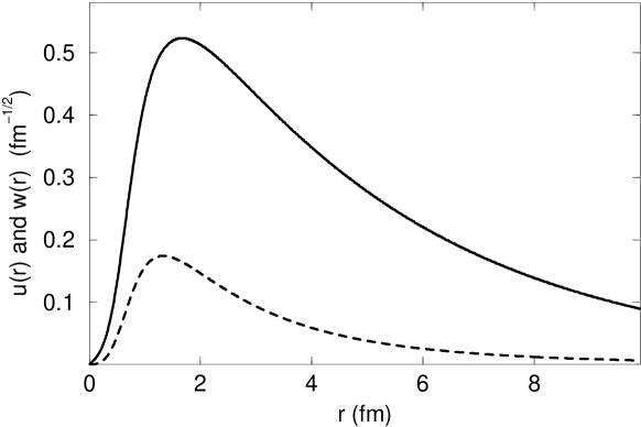
Figure 1: The deuteron reduced radial wave functions $u$ (solid line) and $w$ (dashed) for the Argonne $v_{18}$ potential, as a function of the relative coordinate.

From the wave function, a characteristic size of the deuteron $r_{m}$ is defined as the rms-half distance between the two nucleons :

$$r^{2}_{m}=\frac{1}{4}\int_{0}^{\infty}\left[u^{2}(r)+w^{2}(r)\right]r^{2}dr$$ (7)

Figure 2: The deuteron $S$ wave function in configuration space and in momentum space: $u(r)/r$ and $pu(p)$ (calculated from the Argonne $v_{18}$ potential).

A conspicuous feature of the nucleon-nucleon interaction is the short range repulsion, which leads the radial $S$ wave function $u(r)/r$ to be significantly reduced at distances smaller than approximately 1 fm (see Fig. 2). This introduces a distance scale in the wave function in addition to the overall deuteron size. This small distance behaviour is the subject of most of the experimental and theoretical studies which will be presented in Secs. 4 and 5. As a result of this dip at small $r,$ the Fourier transform $u(p)$ contains a node at approximately 2 fm^-1, as seen also in Fig. 2. The $u$ and $w$ wave functions are given in momentum space by :

$$u(p)=\int_{0}^{\infty}u(r)j_{0}(pr)rdr\quad\hbox{and}\quad w(p)=-\int_{0}^{\infty}w(r)j_{2}(pr)rdr\,.$$ (8)

To conclude this presentation of the size and shape of the deuteron, the densities $|\psi^{0}(\mathbf{x})|^{2}$ and $|\psi^{1}(\mathbf{x})|^{2}$ are illustrated in Fig. 3.

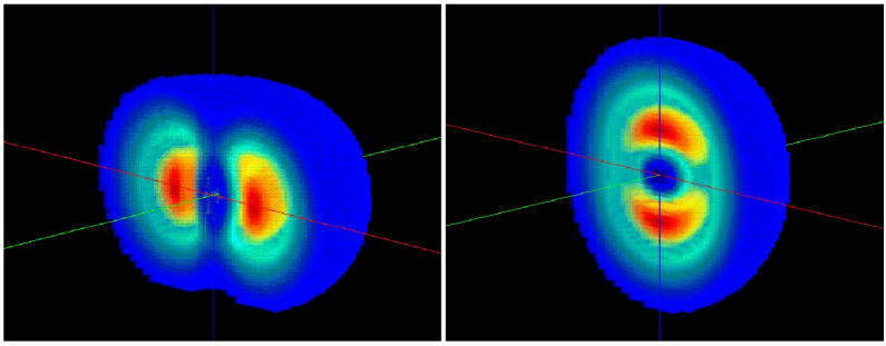
Figure 3: Deuteron densities in $M=0$ (left) and $M=1$ (right) magnetic substates. The red spots correspond to the maximal nucleonic densities, while the dark volumes correspond to lower densities (outer surface is for 10% of maximal density). See [9, 43] for equivalent representations.

In this simple potential model of the deuteron, the magnetic moment of the deuteron is determined entirely by the $D$ state probability $P_{D}$ :

$$\mu_{d}=\mu_{s}-\frac{3}{2}\left(\mu_{s}-\frac{1}{2}\right)P_{D}\,,$$ (9)

where $\mu_{s}=\mu_{n}+\mu_{p}$ is the isoscalar nucleon magnetic moment. The deuteron electric quadrupole moment is also determined from the wave functions:

$$Q_{d}=\frac{1}{\sqrt{50}}\int_{0}^{\infty}w(r)\left[u(r)-\frac{1}{\sqrt{8}}w(r)\right]r^{2}dr\,.$$ (10)

In both cases, these quantities are modified by extensions to the basic potential model (see Sec. 5). In particular the direct relationship between the magnetic moment and the $D$ state probability will be broken by such extensions and, therefore, this probability is not an observable [44].

Since the nuclear force is of finite range, it is easy to determine the asymptotic form of the wave functions

$$u(r)\sim A_{S}e^{-\gamma r}\quad\hbox{and}\quad w(r)\sim A_{D}e^{-\gamma r}\left[1+\frac{3}{\gamma r}+\frac{3}{(\gamma r)^{2}}\right]\quad{\textrm{as}}\;r\rightarrow\infty$$ (11)

where $\gamma\simeq\sqrt{\varepsilon m}$, with $m$ being the reduced $np$ mass and $\varepsilon$ the deuteron binding energy (see Ref. [45] for a relativistic definition of $\gamma$). $A_{S}$ and $A_{D}$ are the asymptotic normalization factors, determined by matching the asymptotic form (11) to the calculated wave functions in the interior region where the potential is nonvanishing. $A_{S}$ and the ratio

$$\eta_{d}=\frac{A_{D}}{A_{S}}$$ (12)

are directly related to observables as discussed in the next section.

3 Static and low energy properties

A review of the measured static properties of the deuteron, together with the low energy neutron proton ($np$) scattering parameters, was given by Ericson and Rosa-Clot [6, 46], who studied in detail their connection with $NN$ potential models. An updated status of the experimental information on the deuteron is given in Table 1 and discussed hereafter.

3.1 Deuteron static properties (experiment)

Table 1: Experimental determinations of the deuteron static properties

Quantity	Most recent	Value
	determination
Mass $M_{d}$	[47, 48]	1875.612762 (75) MeV
Binding energy $\varepsilon$	[49]	2.22456612 (48) MeV
Magnetic dipole moment $\mu_{d}$	[48]	0.8574382284 (94) $\mu_{N}$
Electric quadrupole moment $Q_{d}$	[46, 50, 51]	0.2859 (3) fm2
Asymptotic ratio $\eta_{d}=A_{D}/A_{S}$	[52]	0.0256 (4)
Charge radius $r_{ch}$	[53]	2.130 (10) fm
Matter radius $r_{m}$	[54, 55]	1.975 (3) fm
Electric polarizability $\alpha_{E}$	[56, 57]	0.645 (54) fm3

3.1.1 Mass and binding energy

In the past ten years, significant progress in the precision of the measurement of some atomic masses has been made by comparing cyclotron frequencies of different pairs of ions in a Penning trap. In this way, the deuterium atomic mass is known with a relative precision of $10^{-8}$ [47].

The deuteron binding energy is best determined by measuring the energy of the gamma-rays coming from radiative $np$ capture with thermal neutrons. This energy is now measured to a relative accuracy of $2\times 10^{-7}$, using a crystal diffraction spectrometer [49]. At this precision, even for such a low energy process, some of the earlier work may have to be corrected for relativistic kinematics and the Doppler effect [58].

The binding energy and the mass measurements can be combined for the most precise determination of the neutron mass [49]. The errors on the values reported in Table 1 include the uncertainty in the atomic mass unit $u=931.494013(37)$ MeV [48]. They are well beyond the accuracy of nuclear models.

3.1.2 Magnetic dipole moment

The first measurement of the deuteron magnetic moment was performed by Rabi in 1934 [59], based on a principle [33] already alluded to. From the deflection of an atomic beam in an inhomogeneous magnetic field to the use of molecular beam resonance and other methods, these techniques were continuously improved [60]. Precise measurements of nuclear magnetic resonance frequencies of the deuteron and proton in the HD molecule give the ratio of deuteron to proton magnetic moments. However, the adopted value in Table 1 results from a simultaneous determination of the electronic and nuclear Zeeman energy levels splittings in the deuterium atom, yielding the ratio of deuteron to electron magnetic moments [48].

3.1.3 Electric quadrupole moment

The deuteron was found to possess an electric quadrupole moment in 1939 [61]. This discovery had far reaching consequences: it meant that nuclear forces were not central and were more complex that previously thought. It was to become the best qualitative and quantitative evidence for the role of pions in nuclear physics [6].

In contrast to the case of the magnetic moment which is determined through its coupling to an external applied magnetic field, the quadrupole moment does not couple to an external electric field. One measures instead, in HD or D₂ molecules, the interaction of the deuteron quadrupole moment with the electric field gradient created along the molecular axis by the neighbouring atom. The experiment provides an electric quadrupole interaction constant [50] which must be divided by the theoretically calculated field gradient [51] to obtain the quadrupole moment.

3.1.4 Asymptotic ratio $D/S$

The ratio (12) is deduced from measurements of tensor analyzing powers in sub-Coulomb $(d,p)$ reactions on heavy nuclei by comparison with calculations in the distorted wave Born approximation (DWBA) [52]. The value of $\eta_{d}$ is then directly proportional to the analyzing powers. Other determinations based on $dp$ elastic scattering rely on pole-extrapolation and are somewhat less precise.

3.1.5 Radius and size

The deuteron size may be characterized by a charge radius $r_{ch}$ and by a matter radius $r_{m}$. The latter is defined from the deuteron wave function (7).

Elastic electron scattering has been used since the early fifties [62] to measure the shape of nuclei. This topic will be discussed at length in Sec. 4. At low momentum transfer, the cross section data yield the charge rms-radius of the target nucleus through the relation $r_{ch}^{2}=-6\left.dG_{C}/dQ^{2}\right|_{Q^{2}=0}$ (see Sec. 4.1 for the definition of $G_{C}$). It was demonstrated recently that a precision extraction of the deuteron rms charge radius from electron scattering data requires taking into account the Coulomb distortion of the incoming and outgoing electrons [53]. A new analysis of the world data was then performed, yielding the value in Table 1. The quoted uncertainty combines quadratically the fit statistical error and the dominant systematic error, the latter coming mostly from experimental normalization uncertainties. The usual radiative corrections to electron scattering do not include the contribution of hadronic vacuum polarization, but that effect should be smaller than the present uncertainties when extracting charge radii [63].

The rms charge radius $r_{ch}$ is related to the matter (or rather nucleonic) rms-radius $r_{m}$ [64] by

$$r_{ch}^{2}=r_{m}^{2}+\Delta r_{m}^{2}+r_{p}^{2}+r_{n}^{2}+\frac{3}{4}\left(\frac{\hbar}{m_{p}}\right)^{2},$$ (13)

where $r_{p}=0.862(12)$ fm is the proton charge rms-radius [65] and $r_{n}^{2}=-0.113(5)$ fm² is the neutron charge ms-radius [66]. $\Delta r_{m}^{2}$ is a contribution from non-nucleonic degrees of freedom, close to 0 but with an uncertainty estimated to $\pm 0.01$ fm². The quantity $r_{d}$ given by $r_{d}^{2}=r_{m}^{2}+\Delta r^{2}_{m}$ is usually defined as the deuteron radius. The last term in (13) is of relativistic origin [67]. Note that the above quoted value of $r_{p}$, as extracted from $ep$ elastic scattering, is in slight disagreement ($2\sigma$ difference) with recent Lamb shift measurements [68]. Finally, the theoretical uncertainty in the deuteron radius associated with the correction due to the nucleon finite size has been estimated to about 0.002 fm [69].

The nuclear-dependent correction to the Lamb shift in hydrogen and deuterium atoms is directly proportional to the nuclear mean-square radius. From the isotope shifts in the pure optical frequency of $1S-2S$ two-photon transitions in atomic hydrogen and deuterium, the difference $r_{ch}^{2}-r_{p}^{2}$ of mean-square charge radii for the deuteron and proton is accurately determined [54]. Small corrections due to the deuteron polarizability seem to be under control [55]. Then from (13) and the value of $r_{n}^{2}$, $r_{m}$ is extracted with a better precision than $r_{ch}$ from $ed$ scattering. Our quoted uncertainty is larger than in Ref. [54] because of the use of a larger uncertainty in $r_{n}^{2}$ and the addition of the uncertainty due to $\Delta r_{m}^{2}$.

Taking into account additional small corrections summarized in Ref. [53], the two results given in Table 1 are quite compatible, in the sense that they satisfy Eq.(13). Furthermore, the value of $r_{m}$ follows the expectations from modern $NN$ potentials.

3.1.6 Electric polarizability

The electric polarizability $\alpha_{E}$ characterizes how the deuteron charge distribution can be stretched and acquire an electric dipole moment under the influence of an external electric field. It was determined through elastic scattering of deuterons from ${}^{208}Pb$ well below the Coulomb barrier [56] and extracted from low energy photoabsorption [57]. The two results are slightly incompatible ($2\sigma$ difference). The value in Table 1 is our average.

3.2 Low energy $np$ scattering parameters

The deuteron may also be viewed as a pole in the $S$-matrix describing the $np$ scattering in the coupled ${}^{3}S_{1}$ and ${}^{3}D_{1}$ channels. This $S$-matrix can be experimentally determined from a phase-shift analysis of the scattering data. An extrapolation to negative energies down to the measured deuteron binding energy, either by an effective range expansion [6] or a $P$-matrix approach [70], allows to extract $\eta_{d}$ and $A_{S}$ . The asymptotic ratio $\eta_{d}=0.0254(2)$ is given by the extrapolated mixing parameter $\varepsilon_{1}$ while the asymptotic $S$ state normalization $A_{S}=0.8847(8)$ fm^-1/2 is essentially related to the effective range and thus to the triplet scattering length $a_{t}$ (numerical values from [71]).

3.3 Static properties and the $NN$ potential

All deuteron static properties discussed above are well reproduced by $NN$ potential calculations such as Argonne $v_{18}$, Nijmegen II, Reid93 or CD-Bonn, with the notorious exception of the quadrupole moment, which is always a few percent too low (see also Sec. 5.1). Meson exchange contributions, to be discussed later, must be taken into account for a better agreement with data. The binding energy $\varepsilon$ is taken as a constraint in the determination of all potentials.

Compilations of deuteron static properties caculated with recent $NN$ interaction models appear in [13, 72]. Note that most potentials result in a $D$ wave probability $P_{D}$ between 5.6 and 5.8%, except for the CD-Bonn potential where $P_{D}=4.83\%$.

Various correlations were established between the calculated static properties, independently of the $NN$ potential used. For example, linear relationships between $A_{S}$ and $r_{m}$ [6], or $A_{S}^{2}(1+\eta^{2})$ and $r_{m}^{2}$ [55], and $Q_{d}/A_{S}^{2}$ and $\eta$ [6] were established, the latter depending on the value of the $\pi NN$ coupling constant used in the potential calculation. For more recent potentials, linear relationships between $\mu_{d}$ and $\eta$ on one hand, $Q_{d}$ and $\eta$ on the other hand, are illustrated in [72]. Finally the electric polarizability $\alpha_{E}$ is directly proportional to $r^{2}_{m}$ [55].

4 Elastic electron-deuteron scattering

4.1 Deuteron electromagnetic form factors

Invoking Lorentz invariance, current conservation, parity and time-reversal invariance, the general form of the electromagnetic current matrix element for elastic electron scattering from the spin-1 deuteron can be shown to have the general form [73]:

$$G^{\mu}_{\lambda_{d}^{\prime}\lambda_{d}}(P^{\prime},P) = -\biggl{\{}G_{1}(Q^{2})(\xi^{*}_{\lambda_{d}^{\prime}}(P^{\prime})\cdot\xi_{\lambda_{d}}(P))(P^{\prime}+P)^{\mu}$$ (14)

$$+ G_{2}(Q^{2})\Bigl{[}\xi^{\mu}_{\lambda_{d}}(P)(\xi^{*}_{\lambda_{d}^{\prime}}(P^{\prime})\cdot q)-\xi^{\mu*}_{\lambda_{d}^{\prime}}(P^{\prime})(\xi_{\lambda_{d}}(P)\cdot q)\Bigr{]}$$

$$- G_{3}(Q^{2}){1\over 2M_{d}^{2}}(\xi^{*}_{\lambda_{d}^{\prime}}(P^{\prime})\cdot q)(\xi_{\lambda_{d}}(P)\cdot q)(P^{\prime}+P)^{\mu}\biggr{\}}$$

where $M_{d}$ is the deuteron mass, $P$ and $P^{\prime}$ are the initial and final deuteron four-momenta, $q=P^{\prime}-P$ is the virtual photon four-momentum, $\xi^{\mu}_{\lambda_{d}}(P)$ and $\xi^{\mu*}_{\lambda_{d}^{\prime}}(P^{\prime})$ are the polarization four-vectors for the inital and final deuteron states. The $G_{i}(Q^{2})$ are form factors depending only upon the virtual photon four-momentum; assuming hermiticity, they are real. Since the virtual photon four-momentum is always spacelike for electron scattering, we use the convention $Q^{2}\equiv-q^{2}={\textbf{q}}^{2}-\nu^{2}$.

The current may be expressed in terms of charge monopole, magnetic dipole and charge quadrupole form factors. These are related to the $G_{i}(Q^{2})$’s by:

$$G_{C}(Q^{2}) = G_{1}(Q^{2})+{2\over 3}\eta G_{Q}(Q^{2})$$

$$G_{M}(Q^{2}) = G_{2}(Q^{2})$$

$$G_{Q}(Q^{2}) = G_{1}(Q^{2})-G_{2}(Q^{2})+(1+\eta)G_{3}(Q^{2})$$ (15)

with

$$\eta=\frac{Q^{2}}{4M_{d}^{2}}\;.$$ (16)

These form factors are normalized such that

$$G_{C}(0) = 1\,,$$

$$G_{M}(0) = \frac{M_{d}}{m_{p}}\mu_{d}\,,$$

$$G_{Q}(0) = M_{d}^{2}Q_{d}\;.$$ (17)

The experimental values of $G_{M}(0)$ and $G_{Q}(0)$ are respectively 1.714 and 25.83 (see Table 1).

4.2 Observables

In the Born approximation of a one-photon exchange mechanism and neglecting the electron mass, the cross section for elastic scattering of longitudinally polarized electrons from a polarized deuteron target can be calculated from the current to give in the laboratory frame [74]:

$${d\sigma\over d\Omega} = \frac{\sigma_{M}}{1+\frac{2E}{M_{d}}\sin^{2}\frac{\theta}{2}}\left[v_{L}R_{L}+v_{T}R_{T}+v_{TT}R_{TT}+v_{TL}R_{TL}\right.$$ (18)

$$\qquad\qquad\qquad\qquad+\left.2hv_{T^{\prime}}R_{T^{\prime}}+2hv_{TL^{\prime}}R_{TL^{\prime}}\right]\,,$$

where

$$\sigma_{M}=\left[\frac{\alpha\cos\frac{\theta}{2}}{2E\sin^{2}\frac{\theta}{2}}\right]^{2}$$ (19)

is the Mott cross section, $E$ the electron beam energy, $\theta$ the electron scattering angle and $h=\pm\frac{1}{2}$ the electron helicity. The $R_{l}$ are response functions and the $v_{l}$ kinematical factors are:

$$v_{L} = \left(\frac{Q^{2}}{\mathbf{q}^{2}}\right)^{2}$$

$$v_{T} = \frac{1}{2}\frac{Q^{2}}{\mathbf{q}^{2}}+\tan^{2}\frac{\theta}{2}$$

$$v_{TT} = -\frac{1}{2}\frac{Q^{2}}{\mathbf{q}^{2}}$$

$$v_{TL} = -\frac{1}{\sqrt{2}}\frac{Q^{2}}{\mathbf{q}^{2}}\left[\frac{Q^{2}}{\mathbf{q}^{2}}+\tan^{2}\frac{\theta}{2}\right]^{\frac{1}{2}}$$

$$v_{T^{\prime}} = \left[\frac{Q^{2}}{\mathbf{q}^{2}}+\tan^{2}\frac{\theta}{2}\right]^{\frac{1}{2}}\tan\frac{\theta}{2}$$

$$v_{TL^{\prime}} = -\frac{1}{\sqrt{2}}\frac{Q^{2}}{\mathbf{q}^{2}}\tan\frac{\theta}{2}\;.$$ (20)

For elastic scattering,

$$\frac{Q^{2}}{\mathbf{q}^{2}}=\frac{1}{1+\eta}\,.$$ (21)

Each of the response functions can be written as

$$R_{l}(Q^{2})=\sum^{9}_{i=1}R_{l}(Q^{2},\tau_{i})\tau_{i}$$ (22)

where $l=\{L,T,TT,LT,T^{\prime},LT^{\prime}\}$ and the $\tau_{i}$ are members of the set of the unique deuteron density matrix elements expressed in terms of elements of a spherical tensor $\rho_{kq}$. This set is represented by

$$\tau_{i} = \left\{\rho_{00},\sqrt{3\over 2}\rho_{10},{1\over\sqrt{2}}\rho_{20},\sqrt{3}Re\rho_{22},\sqrt{3}Im\rho_{22},\right.$$ (23)

$$\qquad\left.\sqrt{3\over 2}Re\rho_{11},\sqrt{3\over 2}Im\rho_{11},\sqrt{3\over 2}Re\rho_{21},\sqrt{3\over 2}Im\rho_{21}\right\}\,.$$

The nonvanishing reponse functions for elastic scattering may be written in function of the deuteron form factors :

$$R_{L}(Q^{2},\rho_{00}) = \left(1+\eta\right)^{2}\left[G_{C}^{2}(Q^{2})+\frac{8}{9}\eta^{2}G_{Q}^{2}(Q^{2})\right]$$

$$R_{L}(Q^{2},{1\over\sqrt{2}}\rho_{20}) = -\frac{8}{3}\left(1+\eta\right)^{2}\left[\eta G_{C}(Q^{2})G_{Q}(Q^{2})+\frac{1}{3}\eta^{2}G_{Q}^{2}(Q^{2})\right]$$

$$R_{T}(Q^{2},\rho_{00}) = \frac{4}{3}\eta\left(1+\eta\right)G_{M}^{2}(Q^{2})$$

$$R_{T}(Q^{2},\frac{1}{\sqrt{2}}\rho_{20}) = -\frac{2}{3}\eta\left(1+\eta\right)G_{M}^{2}(Q^{2})$$

$$R_{TT}(Q^{2},\sqrt{3}Re\rho_{22}) = \frac{2}{3}\eta\left(1+\eta\right)G_{M}^{2}(Q^{2})$$

$$R_{TL}(Q^{2},\sqrt{\frac{3}{2}}Re\rho_{21}) = \frac{8}{3}\left(\eta+\eta^{2}\right)^{\frac{3}{2}}G_{M}(Q^{2})\,G_{Q}(Q^{2})$$

$$R_{T^{\prime}}(Q^{2},\sqrt{\frac{3}{2}}\rho_{10}) = -\frac{2}{3}\eta\left(1+\eta\right)G_{M}^{2}(Q^{2})$$

$$R_{TL^{\prime}}(Q^{2},\sqrt{\frac{3}{2}}Re\rho_{11}) = -\frac{8}{3}\eta^{\frac{1}{2}}\left(1+\eta\right)^{\frac{3}{2}}G_{M}(Q^{2})\left[G_{C}(Q^{2})+\frac{\eta}{3}G_{Q}(Q^{2})\right]$$ (24)

It is conventional to write the cross section as

$$\frac{d\sigma}{d\Omega} = \frac{\sigma_{M}}{1+\frac{2E}{M_{d}}\sin^{2}\frac{\theta}{2}}\times\left[A(Q^{2})+B(Q^{2})\tan^{2}\frac{\theta}{2}\right]$$ (25)

$$\quad\times\left[1+\rho_{20}\cdot t_{20}(Q^{2},\theta)+2Re\rho_{21}\cdot t_{21}(Q^{2},\theta)+2Re\rho_{22}\cdot t_{22}(Q^{2},\theta)\right.$$

$$\qquad\left.+h\rho_{10}\cdot t_{10}(Q^{2},\theta)+2hRe\rho_{11}\cdot t_{11}(Q^{2},\theta)\right]$$

where the unpolarized elastic structure functions $A(Q^{2})$ and $B(Q^{2})$ are defined as

$$A(Q^{2}) \equiv v_{L}R_{L}(Q^{2},U)+\frac{1}{2(1+\eta)}R_{T}(Q^{2},U)$$ (26)

$$= G_{C}^{2}(Q^{2})+\frac{2}{3}\eta G_{M}^{2}(Q^{2})+\frac{8}{9}\eta^{2}G_{Q}^{2}(Q^{2})$$

and

$$B(Q^{2}) \equiv R_{T}(Q^{2},U)$$ (27)

$$= \frac{4}{3}\eta\left(1+\eta\right)G_{M}^{2}(Q^{2})\;.$$

Note that the dependence of the cross section on the target polarization is conventionally given by analyzing powers denoted $T_{kq}$; we implicitly use here the equivalence between analyzing powers and recoil deuteron polarizations: $t_{kq}=T_{kq}$ . Defining

$$R_{0}\equiv A(Q^{2})+B(Q^{2})\tan^{2}\frac{\theta}{2}\;,$$ (28)

the tensor polarization observables are

$$t_{20}(Q^{2},\theta) \equiv \frac{1}{\sqrt{2}R_{0}}\left[v_{L}R_{L}(Q^{2},{1\over\sqrt{2}}\rho_{20})+v_{T}R_{T}(Q^{2},{1\over\sqrt{2}}\rho_{20})\right]$$ (29)

$$= -\frac{1}{\sqrt{2}R_{0}}\left\{\frac{8}{3}\eta G_{C}(Q^{2})G_{Q}(Q^{2})+\frac{8}{9}\eta^{2}G_{Q}^{2}(Q^{2})\right.$$

$$\qquad\qquad+\left.\frac{1}{3}\eta\left[1+2(1+\eta)\tan^{2}\frac{\theta}{2}\right]G_{M}^{2}(Q^{2})\right\}$$

$$t_{22}(Q^{2},\theta) \equiv \frac{\sqrt{3}}{2R_{0}}v_{TT}R_{TT}(Q^{2},\sqrt{3}Re\rho_{22})$$ (30)

$$= -\frac{1}{2\sqrt{3}R_{0}}\eta\,G_{M}^{2}(Q^{2})$$

$$t_{21}(Q^{2},\theta) \equiv \frac{1}{2R_{0}}\sqrt{\frac{3}{2}}v_{TL}R_{TL}(Q^{2},\sqrt{\frac{3}{2}}Re\rho_{21})$$ (31)

$$= -\frac{2}{\sqrt{3}R_{0}}\eta\sqrt{\eta+\eta(1+\eta)\tan^{2}\frac{\theta}{2}\,}G_{M}(Q^{2})\,G_{Q}(Q^{2})$$

$$t_{10}(Q^{2},\theta) \equiv \frac{1}{R_{0}}\sqrt{\frac{3}{2}}v_{T^{\prime}}R_{T^{\prime}}(Q^{2},\sqrt{\frac{3}{2}}\rho_{10})$$ (32)

$$= -\frac{1}{R_{0}}\sqrt{\frac{2}{3}}\eta\left(1+\eta\right)\tan\frac{\theta}{2}\sqrt{\frac{1}{1+\eta}+\tan^{2}\frac{\theta}{2}}\,G^{2}_{M}(Q^{2})$$

$$t_{11}(Q^{2},\theta) \equiv \frac{1}{2R_{0}}\sqrt{\frac{3}{2}}v_{TL^{\prime}}R_{TL^{\prime}}(Q^{2},\sqrt{\frac{3}{2}}Re\rho_{11})$$ (33)

$$= \frac{2}{\sqrt{3}R_{0}}\sqrt{\eta+\eta^{2}}\,\tan\frac{\theta}{2}\,G_{M}(Q^{2})\,\left[G_{C}(Q^{2})+\frac{\eta}{3}G_{Q}(Q^{2})\right]$$

There are only two unpolarized elastic structure functions, but three form factors. Since $B(Q^{2})$ depends only on $G^{2}_{M}(Q^{2})$, this form factor can be determined by a Rosenbluth separation of $A(Q^{2})$ and $B(Q^{2})$, or by a cross section measurement at $\theta=180^{\circ}$. $A(Q^{2})$ depends on all three form factors so that only a quadratic combination of $G_{C}(Q^{2})$ and $G_{Q}(Q^{2})$ (the longitudinal part of $A$) can be determined from the unpolarized cross section. A complete separation of the form factors therefore requires the measurement of at least one tensor polarization observable. The possible candidates are $t_{20}$, $t_{21}$ and $t_{11}$, since $t_{22}$ and $t_{10}$ depend only upon $G_{M}^{2}(Q^{2})$ and the unpolarized structure functions. $t_{21}$ and $t_{11}$, being both proportional to $G_{M}(Q^{2})$, are of smaller magnitude than $t_{20}$ and provide in practice a smaller “lever arm” to determine either $G_{C}(Q^{2})$ or $G_{Q}(Q^{2})$ [75]. In addition, the measurement of $t_{11}$ requires intense polarized electron beams, which became available only recently, but offers the simplification of a vector polarization measurement. In all cases so far, this leaves $t_{20}$ as the observable of choice to extract $G_{C}(Q^{2})$ and $G_{Q}(Q^{2})$.

Note that all of the polarization observables depend upon the scattering angle $\theta$ through kinematical factors and $R_{0}(Q^{2},\theta)$. Consequently, the polarization observables measured in different experiments under different kinematical conditions can only be compared if some convention is assumed. Since the first $t_{20}$ measurement [76] was performed close to $\theta=70^{\circ}$, it has been customary to quote the observables at that angle. For experiments not performed at $70^{\circ}$, the observable is extrapolated to this angle, using the known $A(Q^{2})$ and $B(Q^{2})$. Another convention is to use the alternate quantity:

$$\tilde{t}_{20}(Q^{2}) \equiv \frac{1}{\sqrt{2}}\frac{R_{L}(Q^{2},{1\over\sqrt{2}}T_{20})}{R_{L}(Q^{2},U)}$$ (34)

$$= -\frac{\frac{8}{3}\eta G_{C}(Q^{2})G_{Q}(Q^{2})+\frac{8}{9}\eta^{2}G^{2}_{Q}(Q^{2})}{\sqrt{2}\left[G^{2}_{C}(Q^{2})+\frac{8}{9}\eta^{2}G^{2}_{Q}(Q^{2})\right]}\;.$$

The choice of $\tilde{t}_{20}$, which is not strictly speaking an observable, has several advantages. $\tilde{t}_{20}$ is independent of $\theta$, and thus depends only on $Q^{2}$. It is a purely longitudinal quantity, and as such is independent of the magnetic form factor. It has simple properties related to those of the charge and quadrupole form factors (see Sec. 4.4 and Refs. [77, 78]). In particular, the position of nodes in these form factors may be determined directly from a plot of $\tilde{t}_{20}$. Numerically, $\tilde{t}_{20}(Q^{2})$ can be determined from $A(Q^{2})$, $B(Q^{2})$ and $t_{20}(Q^{2},\theta)$ through

$$\tilde{t}_{20}(Q^{2})=\frac{t_{20}(Q^{2},\theta)+\frac{\delta}{2\sqrt{2}}}{1-\delta}\quad\hbox{with}\quad\delta=v_{T}\frac{B(Q^{2})}{R_{0}(Q^{2},\theta)}\,.$$ (35)

As illustrated in Sec. 4.3, in all measurements to date, the ratio $\delta$ is small, so that $\tilde{t}_{20}(Q^{2})$, $t_{20}(Q^{2},\theta)$ and $t_{20}(Q^{2},70^{\circ})$ are not very different from each other. For all these reasons we will use this quantity along with $A(Q^{2})$ and $B(Q^{2})$ for comparison of theoretical predictions to data.

In closing this introduction to $ed$ elastic scattering observables, we refer to App. A for a short discussion of a possible two-photon exchange contribution, especially in view of the large $Q^{2}$ range of available data.

4.3 Review of elastic ed data

The first experiment to measure elastic scattering of electrons on the deuterium was performed at the Stanford Mark III accelerator [79]. Since then, many cross section data points have been measured at various accelerators over the world, with ever increasing precision and at larger and larger momentum transfers [80, 81, 82, 83, 84, 85, 86, 87, 88, 89, 90, 91, 92, 93, 94, 95, 96, 97, 98, 99]. Quite spectacular is the recent achievement of Jefferson Lab to measure $A(Q^{2})$ up to $Q^{2}\simeq 6$ (GeV/c)², making use of a record luminosity of about $5\times 10^{38}$ cm^-2s^-1 to reach cross sections as low as $10^{-41}$ cm²/sr [98]. New measurements of $B(Q^{2})$ for $Q^{2}=$ 0.7 to 1.3 (GeV/c)² from the same experiment will soon be available [100]. The kinematics of all these experiments are illustrated in Fig. 4. Forward angle scattering yields the elastic structure function $A$, while backward angle scattering allows the determination of the elastic structure function $B$. The dashed lines in Fig. 4 indicate what fraction of the cross section corresponds to the contribution of $B(Q^{2})\tan^{2}(\theta/2)$.

Figure 4: Kinematical settings ($\theta$ vs $Q$) for various cross section measurements in $ed$ elastic scattering. The small angle data from SLAC [90] (open circles) and JLab/HallA [98] (filled circles) extend respectively to 10.1 and 12.4 fm^-1, beyond the scale of the horizontal axis. The dashed lines correspond to $B\tan^{2}(\theta/2)/R_{0}=$0.01, 0.1, 0.5, 0.9, 0.99, respectively from bottom to top.

Other experiments measured cross section ratios $ed/ep$ [101, 102].

As already mentionned, the separate determination of the deuteron charge monopole and quadrupole form factors necessitates the measurement of a polarization observable. The observable of choice is $t_{20}$, which is a measure of the relative probabilities of finding the deuteron in magnetic substates $M=-1,0,+1$ after the $ed$ scattering. The Bates Linear Accelerator Center was the first to measure $t_{20}$ [76] and to provide an experimental evidence for the existence of a node of the charge form factor [77]. These double scattering experiments were recently brought to the (up to now) highest possible momentum transfers at Jefferson Lab [103]. For this last experiment as well as for the previously mentioned $A$ measurement [98], electron beams of 100 to 120 $\mu$A were used in conjunction with liquid deuterium targets up to 15 cm long, capable of dissipating 600 W of power deposited by the beam. The combination of a record integrated luminosity, in excess of $10^{9}$ pbarn^-1, and of a large acceptance magnetic channel focusing recoil deuterons onto the high efficiency polarimeter POLDER (see Fig. 5 and App. B) allowed the measurements of $t_{20}$ to be extended up to $Q^{2}\simeq 1.7$ (GeV/c)². The alternative measurement of the tensor analyzing power $T_{20}$, using a polarized target intercepting a stored electron beam, was initiated at Novosibirsk [104, 105, 106], and improved at NIKHEF [107, 108]. New preliminary results from Novosibirsk [109] are also included in this review. On the other hand, the use of a solid cryogenic target (ND₃) in an external electron beam at Bonn resulted in a too low luminosity [110]. The kinematical settings of all these experiments are illustrated in Fig. 6. In all cases, the magnetic contribution to $t_{20}$ is small. A further comparison between these polarization measurements is contained in App. B.

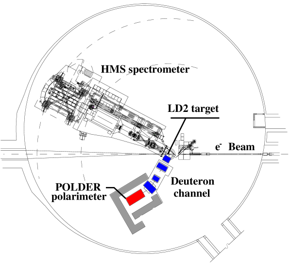
Figure 5: Experimental set-up for the recent $t_{20}$ double scattering experiment [103] in the Hall C (50 m diameter) of Jefferson Lab: $e+d\,\hbox{(LD}_{2})\rightarrow e^{\prime}\,\hbox{(HMS)}+d\,\hbox{(Deuteron}\;\hbox{channel)}$ followed by $d+p\rightarrow(pp)n$ in the POLDER polarimeter.

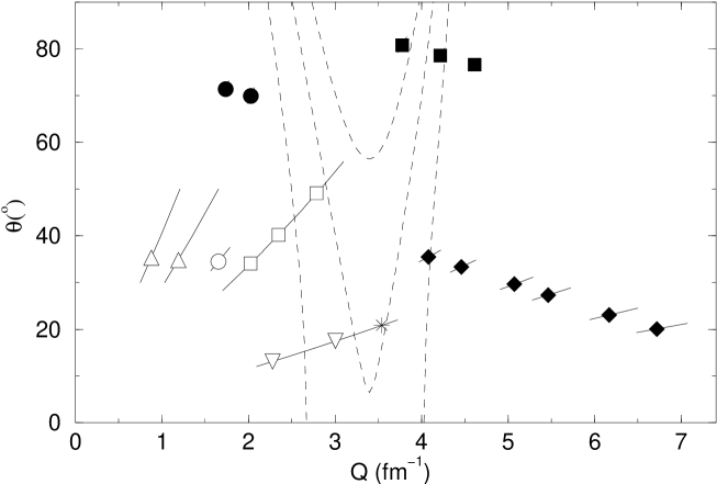
Figure 6: Kinematical settings for measurements of elastic $ed$ tensor polarization observables. Filled symbols for $t_{20}$ measurements of Bates/Argonne [76] (circles), Bates/AHEAD [77] (squares) and JLab/POLDER [103] (diamonds), each at a fixed recoil deuteron angle. Open symbols for $T_{20}$ measurements of Novosibirsk [104, 105] (triangles up), [106] (triangles down), NIKHEF [107] (circle), [108] (squares) and Bonn [110] (star), each at a given electron beam energy. The tilted bars indicate the detector acceptances. The dashed lines are a measure of the small magnetic contribution to $t_{20}$: they correspond to $\widetilde{t}_{20}-t_{20}=0.05,$ 0.1, 0.15, respectively from bottom to top.

The other tensor polarization observables $t_{21}$ and $t_{22}$ (or $T_{22}$) were also measured [77, 103, 107].

Figure 7 shows a good part of the existing data. The $A$ data at low and high $Q^{2}$ will be better illustrated in the figures of Sec. 5, in particular in Figs. 28 and 26. The $t_{21}$ data appears in Fig. 27. In closing this section, let us mention a few inconsistencies in this data set in the light of recent measurements. The $A(Q^{2})$ Cambridge [87] and Bonn [94] data are very probably too low, since both recent measurements at Jefferson Lab [98, 99] agree with the “higher” trend already given by the SLAC data [90]. Still, as apparent in Fig. 28, these two JLab measurements differ from each other (10-15%) in the region $Q^{2}=1$ to 2 (GeV/c)². For a comparative discussion of these two independent experiments, see [111]. The $t_{20}$ (or $T_{20}$) data are necessarily less precise than cross section measurements and naturally exhibit some scatter. Although all data points are compatible with parameterizations such as discussed below, there are some trends between different data sets. No parameterization or model can accomodate both the Bates [77] and NIKHEF [108] data sets: one or the other is too low, or both are. The same Bates data are also systematically lower than both the JLab [103] and the preliminary Novosibirsk data [109], and the precise low $Q^{2}$ NIKHEF point [107] is lower than many theoretical expectations. Though these scatters are compatible with the quoted experimental errors, they demonstrate (together with the theoretical models to be discussed) a need for a more accurate measurement in the region $Q=3$ to 4.5 fm^-1. Finally, the Bates $t_{22}$ data point at $Q\simeq 3.8$ fm^-1 [77] is obviously wrong, but the authors did not find a correlation between $t_{20}$ and $t_{22}$ in their analysis .

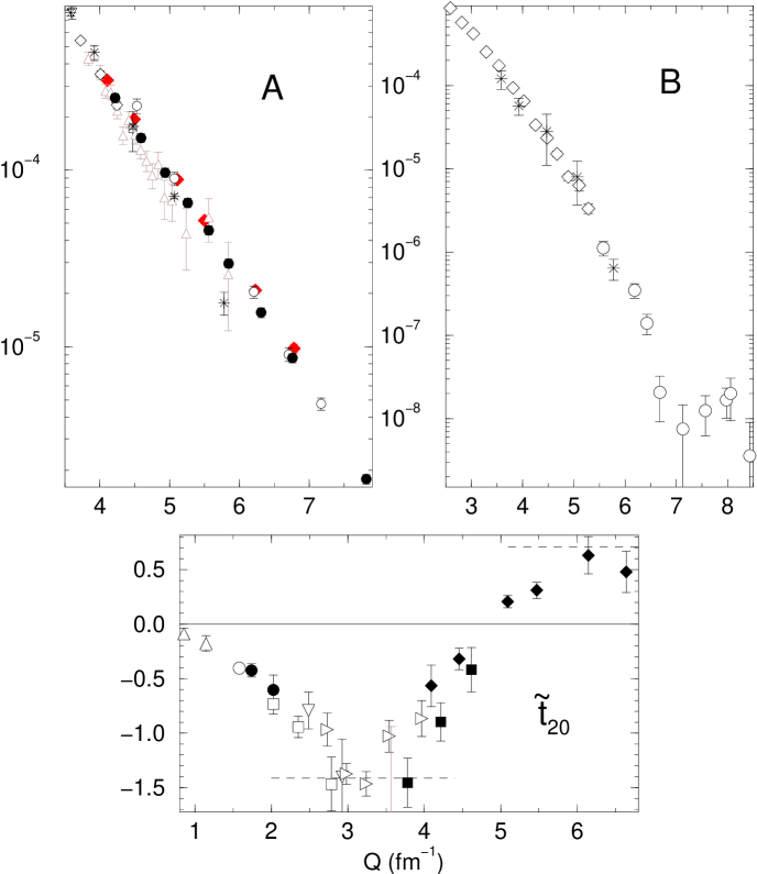
Figure 7: Elastic $ed$ scattering observables. The $A$ data are from Cambridge [87] (triangles), SLAC [90] (open circles), Bonn [94] (stars), Saclay [97] (open diamonds), JLab/HallA [98] (full circles) and JLab/HallC [99] (full diamonds). The $B$ data are from Saclay [95] (diamonds), SLAC [96] (circles), Bonn [94] (stars). For $t_{20}$ data legend, see Fig. 6.

4.4 Empirical features of form factors

The three deuteron electromagnetic form factors may be calculated at a fixed value of $Q^{2}$ from measurements of $A$, $B$ and $t_{20}$. The magnetic form factor $G_{M}$ is readily available from the $B$ measurements, while the two charge form factors $G_{C}$ and $G_{Q}$ are determined from $v_{L}R_{L}(Q^{2},U)\equiv A_{L}=A-B/2(1+\eta)$ (26) and $\tilde{t}_{20}$ (34,35). The resolution of these equations is most simply described in Ref. [78], together with a discussion of possible ambiguities in the choice of different solutions in the $Q$-regions where $\tilde{t}_{20}$ reaches its extrema. This procedure allows a direct comparison of theoretical models with the form factors, instead of observables, but it is limited to the domain where the three observables are measured, which is $Q=0-7$ fm^-1($Q^{2}\leq 1.8$ (GeV/c)²).

The most striking result is an experimental determination of the node of $G_{C}$, at $Q=4.21$$\pm 0.08$ fm^-1 [78], which corresponds to $\tilde{t}_{20}$$=-1/\sqrt{2}$ . This behaviour of $G_{C}$, though expected from most models, could not have been seen with cross section measurements only. The exact location of this node is sensitive to the strength of the $NN$ repulsive core (in the impulse approximation, it is connected to the node of $u(p)$ in Fig. 2) and to the size of relativistic corrections and of the isoscalar meson exchange contributions. A secondary maximum is also determined from the data [103]. Thus, like any other nucleus, the deuteron appears to have a charge form factor with an oscillatory diffractive pattern. Unlike other nuclei, the sign of this form factor is determined as well.

The quadrupole form factor $G_{Q}$ exhibits a monotonous exponential fall-off, and its first node, corresponding to the yet unobserved second node of $\tilde{t}_{20}$, is expected beyond $Q=7$ fm^-1.

Finally the magnetic dipole form factor $G_{M}$ has a node at $Q=7.2$$\pm 0.3$ fm^-1, determined by $B$ data [96] and in a lesser extent by $t_{21}$ data [103]. The position of this node is very sensitive to small non-nucleonic components in the deuteron wave function, to nucleon-nucleon components of relativistic origin, as well as to the description of the $\rho\pi\gamma$ contribution to be discussed in the next section.

The three form factors were parameterized in three different ways: rational fractions (I), sum of Lorentzian functions in an helicity basis (II) and sum of Gaussian functions (III) [78], fitting directly the measured observables, i.e. differential cross sections and polarizations. Figure 8 gives a representation of the form factors with an updated version of parameterization I, taking into account the preliminary $T_{20}$ data of Ref. [109]. The data base and the parameterizations are available in [112].

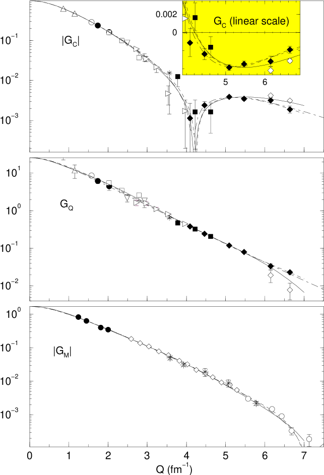
Figure 8: Deuteron form factors $G_{C}$, $G_{Q}$ and $G_{M}$ as a function of $Q$ (updated from Fig. 1 of Ref. [78]). The data for $G_{C}$ and $G_{Q}$ correspond to $t_{20}$ (or $T_{20}$) measurements (see legend of Fig. 6), including new preliminary results from [109] (triangles right). The open diamonds correspond to a second solution of the equations $G_{C},G_{Q}=f(A,B,t_{20})$ [78]. The $G_{M}$ data correspond to the $B$ measurements indicated in Fig. 7, with the addition of [93] (full circles). The curves are from parameterizations I (solid line), II (dot-dashed) and III (short dashed) discussed in the text.

Another representation of the experimental knowledge of the deuteron form factors is given in Fig. 9, where the contributions from each of them to the elastic structure function $A$ are given, calculated using parameterization I.

Figure 9: $A(Q^{2})$ (solid curve) and the contributions from $G_{C}$ (long dashed), $G_{Q}$ (dashed) and $G_{M}$ (dotted), from parameterization I. Above 1.3 (GeV/c)², the statistical significance of the data is such that the crossing of the $G_{C}$ and $G_{Q}$ contributions, corresponding to $\tilde{t}_{20}=1/\sqrt{2}$, is not firmly established.

5 Theoretical issues

The different classes of theoretical models of the deuteron electromagnetic form factors are presented here, illustrated with the most recent calculations on the subject. A summary of earlier theoretical work on the subject may be found for instance in [77, 97]. In all figures of this section, the data legend is the same as in Sec. 4.3.

5.1 Deuteron elastic form factors in the simple potential model

Once the wave functions for a given potential model are obtained as discussed in Sec. 2, the electromagnetic form factors may readily be calculated in the nonrelativistic impulse approximation (NRIA) using a well established formalism [113, 114]. The virtual photon can couple to any of the two nucleons, so that the isoscalar combinations $G_{E,M}^{S}$ of the nucleon form factors (NEMFF), defined in App. C, factorize to yield [3, 115]:

$$G_{C}(Q^{2}) = G_{E}^{S}(Q^{2})\times C_{E}(u,w;Q^{2})$$

$$G_{Q}(Q^{2}) = G_{E}^{S}(Q^{2})\times C_{Q}(u,w;Q^{2})$$

$$G_{M}(Q^{2}) = G_{E}^{S}(Q^{2})\times C_{L}(u,w;Q^{2})+G_{M}^{S}(Q^{2})\times C_{S}(u,w;Q^{2})$$ (36)

The $C$ functions are integrals of quadratic combinations of $u$ and $w$. In this NRIA, the ratio $G_{Q}/G_{C}$, and thus $\widetilde{t}_{20}$, are independent of the nucleon form factors. The coupling of the virtual photon to the moving nucleon charges and to the nucleon spins both contribute the magnetization in $G_{M}$, giving rise to the two terms in (36). The elastic structure functions $A(Q^{2})$, $B(Q^{2})$ and $\tilde{t}_{20}(Q^{2})$ are illustrated in Fig. 10 for a variety of phenomenological potentials [116, 117, 42], using the MMD parameterization of the nucleon form factors (see App. C).

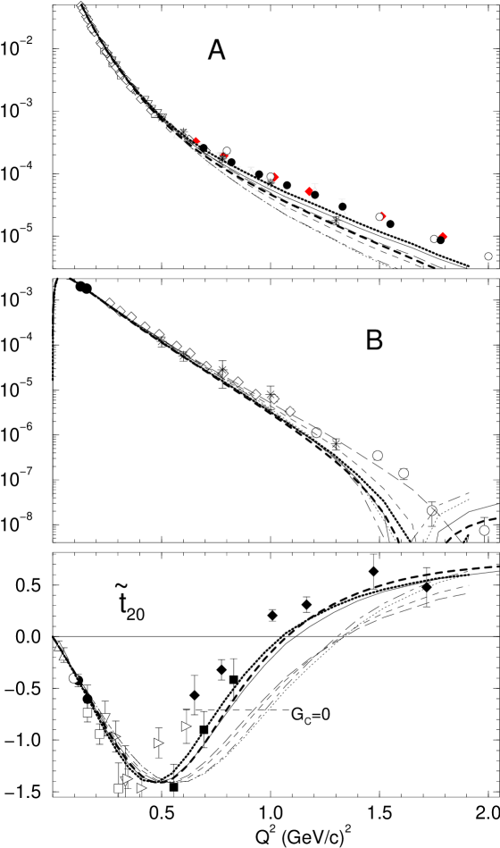
Figure 10: Elastic $ed$ scattering observables for a variety of phenomenological potentials in the NRIA: Bonn-A (dotted curve), Bonn-B (dashed), Bonn-C (long-dashed), Bonn Q (dot-dashed), Reid-SC (thick dotted), Paris (solid) and A-$v_{18}$ (thick dashed). NEMFF: MMD.

In all cases the calculations agree with one another and with the data up to $Q^{2}\sim 0.5$ (GeV/c)² but diverge at higher $Q^{2}$. The low $Q^{2}$ behaviour of the form factors is not determined with the same precision for each of them. Since the forward cross sections at low $Q^{2}$ depend mostly on $G_{C}$, the slope of this form factor at $Q^{2}=0$ is determined to about 1% (see Sec. 3.1.5). The slope of $G_{M}$ at the origin is determined by backward cross sections and is known to about 5%. In contradistinction, the slope of $G_{Q}$ is known to only 15%, in the absence of very precise $t_{20}$ measurements at low $Q^{2}$. Still this slope is model dependent. To illustrate this point, we define the reduced quantity

$$\tilde{t}_{20R}(Q^{2})=-\frac{3}{\sqrt{2}Q_{d}Q^{2}}\tilde{t}_{20}(Q^{2})$$ (37)

and show its low $Q^{2}$ behaviour in Fig. 11.

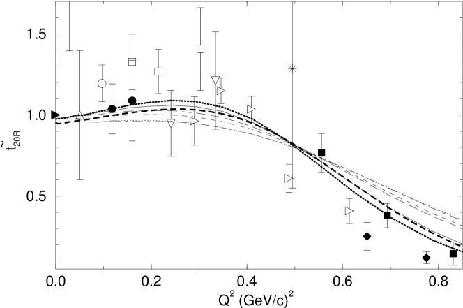
Figure 11: $\tilde{t}_{20R}$ from (37) for a variety of phenomenological potentials in the NRIA. Same legend as Fig. 10. The solid right triangle results from the definition of $\tilde{t}_{20R}$.

At $Q^{2}=0$, one gets

$$\tilde{t}_{20R}(0)=\frac{G_{Q}(0)}{Q_{d}M_{d}^{2}}\quad\hbox{and}\quad\frac{\tilde{t}^{\prime}_{20R}(0)}{\tilde{t}_{20R}(0)}=\frac{G^{\prime}_{Q}(0)}{G_{Q}(0)}-G^{\prime}_{C}(0)+\frac{G_{Q}(0)}{12M^{2}_{d}}\,.$$ (38)

$G_{Q}(0)$ is the model calculation of the quadrupole moment. The slope $\tilde{t}^{\prime}_{20R}(0)$ is rather small, due to an approximate cancellation between the first two terms, the third one being significantly smaller. In this connection, it is instructive to list in Table 2 the model dependences of these various slopes. The value of the quadrupole form factor varies substantially for these calculations and is always smaller than the experimental value of 25.8 (17). All of the Bonn calculations and the Reid-SC calculation yield the same value for the derivative of the charge form factor and the same of is true of the derivative of the quadrupole form factor with the exception of Bonn A. Therefore the spread in $\tilde{t}^{\prime}_{20R}(0)$ for this latter set comes only from the variation in the value of the quadrupole form factor. However, this may not be the case in general.

Table 2: Dependence upon various potentials of the quantities appearing in Eq.(38). Slopes in (GeV/c)^-2.

Potential	$G_{Q}(0)$	$\widetilde{t}_{20R}(0)$	$G^{\prime}_{Q}(0)$	$G^{\prime}_{C}(0)$	$\widetilde{t}^{\prime}_{20R}(0)$
Bonn A	24.8	.960	-506	-18.1	-1.69
Bonn B	25.1	.972	-464	-18.1	0.25
Bonn C	25.4	.983	-464	-18.1	0.47
Bonn Q	24.7	.956	-464	-18.1	-0.06
Reid SC	25.2	.976	-464	-18.1	0.32
Paris	25.2	.976	-453	-18.5	1.09
A-$v_{18}$	24.1	.932	-444	-18.1	0.28

The increasing disagreement between these simple calculations and the data at higher $Q^{2}$ indicates that this approach does not contain all of the necessary physical degrees of freedom and/or that since the momentum transfer approaches and then surpasses the mass of the nucleon, it is necessary to consider the impact of special relativity on the calculation of the deuteron elastic structure functions. We will now consider the first of these possibilities.

5.2 Limitations of the simple potential model

For many applications in nuclear physics, the phenomenological potential approach is completely adequate and provides a good description of various phenomena. Its limitations were seen, however, by considering the calculation of electromagnetic properties of the deuteron in the preceding section.

The inclusion of electromagnetic interactions with the two-nucleon system imposes the requirement that the electromagnetic current matrix elements satisfy the continuity equation

$$\nabla\cdot<\Psi_{f}|\widehat{\mathbf{J}}(\mathbf{x})|\Psi_{i}>+\frac{\partial}{\partial t}<\Psi_{f}|\hat{\rho}(\mathbf{x})|\Psi_{i}>=0$$ (39)

where $\widehat{\mathbf{J}}(\mathbf{x})$ and $\hat{\rho}(\mathbf{x})$ are the current and charge density operators. The operators must then satisfy

$$\nabla\cdot\widehat{\mathbf{J}}(\mathbf{x})-i\left[\hat{\rho}(\mathbf{x}),\hat{H}\right]=0\,.$$ (40)

Since either of the nucleons can be charged, the charge density operator is

$$\hat{\rho}=\hat{\rho}_{1}+\hat{\rho}_{2}\,,$$ (41)

while the current density takes the general form

$$\widehat{\mathbf{J}}=\widehat{\mathbf{J}}_{1}+\widehat{\mathbf{J}}_{2}+\widehat{\mathbf{J}}_{ex}\,,$$ (42)

where $\hat{\rho}_{i}$ and $\widehat{\mathbf{J}}_{i}$ are the charge and current densities for particle $i$ and $\widehat{\mathbf{J}}_{ex}$ is a possible additional contribution to the current density.

The current of a free charged particle must satisfy the continuity equation, which implies

$$\nabla\cdot\widehat{\mathbf{J}}_{i}(\mathbf{x})-i\left[\hat{\rho}_{i}(\mathbf{x}),\hat{T}_{i}\right]=0\,.$$ (43)

Using this with (40), (41) and (42) gives

$$\nabla\cdot\widehat{\mathbf{J}}_{ex}(\mathbf{x})-i\left[\hat{\rho}(\mathbf{x}),\hat{V}\right]=0\,.$$ (44)

Since $\hat{\rho}_{i}$ is proportional to $(1+\tau_{3}^{(i)})$ and the two-nucleon potential $\widehat{V}$ has terms proportional to $\tau^{(1)}\cdot\tau^{(2)}$, the second term in (44), proportional to $(\tau^{(1)}\wedge\tau^{(2)})_{3}$, does not vanish and $\widehat{\mathbf{J}}_{ex}$ must be nonzero. In addition, since $\widehat{V}$ involves the coordinates of both nucleons, the current $\widehat{\mathbf{J}}_{ex}$ must also depend upon both sets of coordinates and is therefore a two-body operator. The physical origin of this contribution to the current comes from the fact that the two-nucleon potential contains terms corresponding to the exchange of charge between the nucleons, which must in turn give rise to an associated current. These two-body currents are called exchange or interaction currents.

Equation (44) is a symmetry constraint on the theory. It cannot, however, be used to uniquely determine $\widehat{\mathbf{J}}_{ex}$ since divergenceless pieces can be added to any current satisfying (44) without modifying the constraint. A unique prediction of the current therefore requires that the underlying dynamics of the interaction be specified. Viewing the nuclear force in a meson-exchange model, these two-body currents are naturally associated with contributions that involve the exchange of mesons [118]. Now that it is generally accepted that quantum chromodynamics (QCD) is the correct description of the strong force at the scales of interest here, these currents must ultimately be associated with the exchange of quarks.

This discussion leads to a consistent treatment in the context of a nonrelativistic treatment of the two-nucleon problem. However, any attempt to implement this approach in a manner that is applicable to the existing data, for instance to the case of elastic electron-deuteron scattering, leads directly to consistency problems. One of the most elementary indications of this problem arises from the necessity of including electromagnetic form factors for the nucleons. At low momentum transfers, these form factors differ from their static values by terms of order $Q^{2}/m_{D}^{2}$. Since the dipole mass $m_{D}$ is of similar magnitude as the nucleon mass, this is of leading relativistic order $v^{2}/c^{2}$. Whenever the presence of the nucleon electromagnetic form factors has an appreciable effect on the calculations of the deuteron form factors, some effects of relativistic order are already included. It then becomes necessary to consider whether there are other relativistic effects of similar size that can appreciably modify the calculations. In fact, there are many such effects arising from Lorentz boosts and exchange currents that become increasingly important in the calculations of deuteron form factors as the four-momentum transfer increases. For this reason it is necessary to consider how relativity can be introduced consistently in models of the deuteron. For this purpose, we will assume that the deuteron is adequately described by nucleons and mesons.

5.3 Construction of relativistic models

The requirement of any truly relativistic model is that it must satisfy Poincaré covariance: it must be covariant with respect to Lorentz boosts, spatial rotations and space-time translations. This can be imposed by requiring that the the operators which act as generators of these transformations satisfy the Lie algebra of this group:

$$\left[J^{i},J^{j}\right]=i\epsilon^{ijk}J^{k},\qquad\left[K^{i},K^{j}\right]=-i\epsilon^{ijk}J^{k}$$ (45)

$$\left[J^{i},K^{j}\right]=i\epsilon^{ijk}K^{k}$$ (46)

$$\left[P^{\mu},P^{\nu}\right]=0$$ (47)

$$\left[K^{i},P^{0}\right]=-iP^{j},\qquad\left[J^{i},P^{0}\right]=0$$ (48)

$$\left[K^{i},P^{j}\right]=-i\delta^{ij}P^{0},\qquad\left[J^{i},P^{j}\right]=i\epsilon^{ijk}P^{k}$$ (49)

where $J^{i}$ are the three angular momentum operators that generate rotations, $K^{i}$ are the generators of the three Lorentz boosts and $P^{\mu}$ is a four-vector containing the energy and momentum operators that generate space-time translations. This differs from the corresponding algebra for the Galilean transformations in only two commutators. The differing commutators for the Galilean transformations are:

$$\left[K^{i}_{G},K^{j}_{G}\right]=0$$ (50)

and

$$\left[K^{i}_{G},P^{j}\right]=-i\delta^{ij}M$$ (51)

where $K^{i}_{G}$ are the generators of the Galilean “boosts” and $M$ is the mass operator. The first of these implies that Galilean boosts commute whereas Lorentz boosts do not. The second is the source of the dynamical complexity of relativistic models and theories. While the commutators for the Galilean boosts and the three-momentum operators are proportional to the mass, the corresponding commutators for the Poincaré group are proportional to the energy operator, that is the Hamiltonian. Since the Hamiltonian contains the interactions between the constituents of the system, the first commutator of (49) implies that the Lorentz boost operators or three-momentum operators must also be dependent upon the interaction.

There are two basic approaches to constructing Poincaré invariant models. We will start with the most familiar of these, quantum field theory.

5.3.1 Quantum field theory

The starting point of a quantum field theory is a Lagrangian that is constructed to satisfy all of the required symmetries, including Poincaré invariance. By nature field theories have an infinite number of degrees of freedom. Canonical quantization is performed by constructing the Hamiltonian, finding the generalized position and momentum in terms of the fields, writing the fields as an expansion in terms of creation and annihilation operators, and then imposing canonical equal time commutation (anticommutation) relations on the canonical variables. This yields commutation (anticommutation) relations for the creation and annihilation operators. An immediate consequence is that the fields commute (anticommute) for all spacelike intervals, implying that events occuring at spacelike separations cannot be causally connected. This is the property of microscopic causality or microscopic locality. It should be noted here that microcausality results from imposing the commutation (anticommutation) relations on any spacelike hypersurface.

The structure of field theories is very complex due to the presence of an infinite degrees of freedom. Since the Hamiltonian of an interacting system links states containing different numbers of particles, and the time-evolution operator of the system is given by the imaginary exponential of the interacting Hamiltonian, the interacting system contains contributions with any number of particles, from zero to infinity. Practical calculations in field theory, with the exception of numerical approaches such as lattice QCD, must then introduce some method of truncating the collection of configurations contributing to the calculation. The most familiar approach to this problem is Feynman perturbation theory. Here, various configurations are carefully arranged such that all quantities contributing to a process, such as free propagators and vertex functions, are individually covariant with respect to noninteracting Lorentz transformations. The truncation then requires that there be some plausible scheme for systematically organizing contributions in order of their relative importance. For example, in the classic case of quantum electrodynamics where the coupling constant is small, the terms are ordered in powers of the coupling constant and truncated at some finite order.

The drawbacks of quantum field theory for constructing models such as for $NN$ interactions are related to complexities and calculational difficulties. Most of our knowledge of field theory is based on perturbation theory and there is no a priori method for determining the radius of convergence (if any) for a given field theory. For strong coupling theories, it is no longer plausible to construct a perturbation scheme in terms of simple counting of coupling constants and infinite sets of contributions must be summed. In practice, the coupling of the infinite sets of states, or $n$-point functions, must be truncated if there is to be any hope of calculation. Thus some physically reasonable scheme for truncation must be proposed. However, the truncation of the theory will usually violate some symmetries of the full theory such as crossing symmetries, covariance or current conservation. Local effective theories with the appropriate symmetries may also be nonrenormalizable. Model calculations may also include phenomenological elements such as form factors that are not calculated within the context of the field theory. This also leads to problems of consistency within the model and may also violate symmetries.

5.3.2 Hamiltonian dynamics

Although Dirac was one of the founders of quantum field theory, he soon became disillusioned with its complexity and the difficulties associated with the unavoidable infinities. He continued for most of the rest of his life to seek an alternative to quantum field theory. He assumed that the problems with field theory were related to starting from an unsatisfactory relativistic classical theory. He pointed to an alternate approach, starting with a theory with a fixed number of degrees of freedom, as is done with the nonrelativistic Schrödinger equation. This led to relativistic constraint dynamics [119]. In this approach, the dynamics of a model system is determined by choosing a mass operator which contains an instantaneous interaction as in the nonrelativistic potential theory. This basic dynamics contains a finite number of particles and has a corresponding Hilbert space when quantized. Covariance is imposed by constructing a unitary representation of the inhomogenous Lorentz transformations with generators that satisfy the commutation relations of the Poincaré group. The wave functions have the same probabilistic interpretation as in nonrelativistic quantum mechanics, but microscopic causality is not respected: the theory must be constructed to respect the physical requirement of cluster separability or macroscopic locality.

There are at least three different approaches for the quantization of such models. The first is the traditional method of quantizing along constant time surfaces (called instant form) where the evolution of the system is the usual time evolution which is normal to the constant-time hypersurface. The second is to quantize along spacelike surfaces with constant interval (called point form). The evolution of the system is then along a new coordinate normal to these surfaces. The third of these is to quantize along the light cone with evolution along the coordinate $x^{+}=x^{0}+x^{3}$. Since all these choices describe surfaces with spacelike separations (or the infinite momentum limit of such a surface in the light-cone case), they are also consistent with microscopic causality for field theories, which may also be quantized along these surfaces.

Particularly useful in the Hamiltonian dynamics is the fact that a careful construction of the mass operator can lead to equations of motion of the same form as the two-body Schrödinger equation. It is therefore possible to use, without modification, nonrelativistic potentials that have been fitted to describe $NN$ scattering .

The drawbacks are related to the choice of the interaction without specification of any underlying dynamical content. As a result, quantities such as electromagnetic currents can be constrained by the structure of the theory, but can not be uniquely determined from the interaction dynamics.

We will now proceed to a discussion of various approaches used in constructing relativistic calculations of the elastic electromagnetic form factors for the deuteron.

5.4 $v/c$ expansions

This approach is actually a hybrid of field theory and Hamiltonian dynamics. It assumes that the basic dynamical content of the deuteron is nonrelativistic and that the necessary relativistic effects can be described as corrections to the nonrelativistic current matrix elements as an expansion in $v/c$ [120, 121, 122].

The nucleon-nucleon interaction is taken to be a standard nonrelativistic potential with parameters determined by fitting to the nucleon-nucleon scattering data and to the deuteron binding energy. It is assumed that the potential is, at least in part, represented by a one-meson-exchange model, since the meson degrees of freedom are necessary to construct two-body exchange currents from simple Feynman diagrams and for constructing corrections due to retardation of meson propagators. Examples of the required two-body interaction currents are represented in the diagrams of Fig. 12. Diagram (a) represents a contribution due to coupling of the photon to the current of an exchanged meson, which, because of $G$-parity, does not apply to isoscalar transitions such as $ed$ elastic scattering. Diagram (b) is a so called pair current that arises due to the projection of the interactions onto the positive-energy space only. Contributions that couple to the negative energy part of the nucleon propagator must then be included in the current. Diagram (c) is a retardation correction. Since nonrelativistic wave functions are single-time wave functions, diagrams corresponding to the absorption of a photon while the meson is in flight are not included in the impulse approximation and must be included in the current. Retardation corrections can also be associated with retarded meson propagation in any of the other diagrams in this figure. Derivative couplings of the mesons to the nucleons can also give rise to contact interactions of the type shown in diagram (d), which is isovector and does not apply to $ed$ elastic scattering. It is also possible for a photon that is absorbed by an exchanged meson to excite the meson. An example is the $\rho\pi\gamma$ exchange current which is commonly included in calculations of elastic electron-deuteron scattering. Such a current is represented by diagram (e).

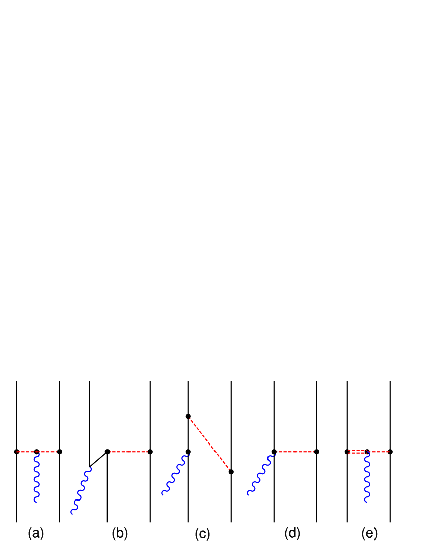
Figure 12: Two-body currents arising in the $v/c$ expansions (see text for explanations).

Relativity is imposed by requiring that the currents and interactions are consistent with operator commutators of Poincaré invariance to some order in $v/c$. The dependence of the boost operators on the interaction also gives rise to interaction currents in addition to those characterized above. This approach guarantees that the interaction model can be very well constrained by data but its application can become technically complicated. In addition, the expansion in $v/c$ must fail at some value of momentum transfer.

The calculations shown here are from a recent paper by Arenhövel, Ritz and Wilbois (ARW) [123]. This paper is an extension of earlier work [116, 124] that included relativistic corrections for the charge and quadrupole form factors, but not the magnetic. Although there is an extensive literature on the subject, as nicely summarized in [123], only that paper and the earlier work of Tamura [125] take into account all leading order terms including the Lorentz boost of the deuteron center of mass. The need for a realistic one-boson-exchange potential leads ARW to use the Bonn OBEPQ models, which may however not have the same precision in describing $NN$ scattering data as more recent, but more phenomenological, potentials. Finally the Galster dipole parameterization for the nucleon electromagnetic form factors was used.

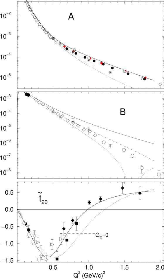
Figure 13: Elastic $ed$ scattering observables calculated with the $v/c$ expansion [123]: NRIA with the Bonn OBEPQ-B potential (dotted curve); same plus all relativistic corrections to leading order (dashed); all of the former plus the $\rho\pi\gamma$ exchange current (solid). NEMFF: Galster.

Figure 13 shows the observables $A(Q^{2})$, $B(Q^{2})$ and $\tilde{t}_{20}(Q^{2})$ for this model. Three curves are shown for each observable, the impulse approximation (NRIA), the impulse approximation plus all relativistic corrections to leading order, and all of the former plus the $\rho\pi\gamma$ exchange current. The $\rho\pi\gamma$ exchange current is purely transverse and is not required or constrained by the interaction model, but is the longest range isoscalar current of this type.

The elastic structure function $A(Q^{2})$ for the impulse approximation is substantially below the data. The inclusion of the various relativistic corrections brings the calculation into much better agreement with the data, while the addition of the $\rho\pi\gamma$ exchange current has only a very small effect.

In the case of the magnetic structure function $B(Q^{2})$, the NRIA again is below the data and has a diffraction minimum at lower $Q^{2}$ than indicated by the data. The addition of the relativistic corrections increases the size of the calculated structure function and appears to move the diffraction minimum above the value indicated by the data. The addition of the $\rho\pi\gamma$ exchange current again increases the size of the structure function to a value considerably above the data and presumably pushes the diffraction minimum to even higher values. We will return later to the question of the effect of this exchange current on the magnetic structure function, in the context of field-theoretical models.

For the polarization structure function $\tilde{t}_{20}(Q^{2})$, the NRIA is above the data for small $Q^{2}$ below its minimum, and below at $Q^{2}$ above the minimum. The addition of the relativistic corrections brings the calculation into much better agreement with the observed node of $G_{C}$ and consequently with the data. The $\rho\pi\gamma$ exchange current only has a very small effect on this observable which is purely longitudinal.

The examination of the figures in Ref. [123] shows that the various corrections to the NRIA are not small, they tend to be of similar magnitude, and they contribute to the deuteron form factors with varying signs. As a result, any calculation that includes some, but not all, of these corrections, is questionable.

These calculations clearly indicate that relativistic effects, that is meson-exchange contributions and genuine relativistic corrections, are important even for relatively small momentum transfers. The domain of validity of this approach is thus limited, probably to $Q^{2}\leq 1$ (GeV/c)², though it may lead in some instances to a satisfactory description of the data up to 2 (GeV/c)² [42]. The study of the validity of the two-nucleon description of the deuteron down to very small internucleon distances, together with new data becoming available from Jefferson Lab, make mandatory the consideration of fully relativistic models.

5.5 Relativistic constraint dynamics

Figure 14 shows three recent calculations the deuteron elastic structure functions. Note that in this and following figures, the different observables are not shown in the same $Q^{2}$ range, following the available data. This should be kept in mind for a meaningful comparison of models to data. The calculation of Allen, Klink and Polyzou (AKP) [126] uses the Argonne $v_{18}$ potential for an interaction and is quantized in point form. The calculation of Lev, Pace and Salmè (LPS) [72, 127] uses the Nijmegen II potential and is quantized in front form. The calculation of Forest and Schiavilla (FS) [128] uses the Argonne $v_{18}$ potential and is quantized in instant form. These three calculations involve three different approaches to construct currents. AKP and LPS use different procedures for constructing currents from the single-nucleon current without including any interaction dependent two-body currents. FS assume that the potential is of one-boson-exchange origin and construct the various currents as in the $v/c$ expansions, but without performing this expansion. These calculations show considerable variation in all three observables. Although the FS calculation works quite well for all of them, it is clear that no consensus has been reached concerning consistent techniques for the construction of currents in this framework.

Figure 14: Elastic $ed$ scattering observables calculated with the Hamiltonian constraint dynamics. AKP [126], NEMFF: MMD (solid curve); LPS [127], GK85 (dashed); FS [128], H (dot-dashed).

5.6 Field theoretical models

5.6.1 The Bethe-Salpeter equation

The oldest of the field-theoretical treatments of the two body-problem is due to Bethe and Salpeter [129]. The physical content of the Bethe-Salpeter equation can be easily understood by considering the two-body scattering matrix $\mathcal{M}$. Figure 15 represents the Feynman expansion of the scattering matrix $\mathcal{M}$

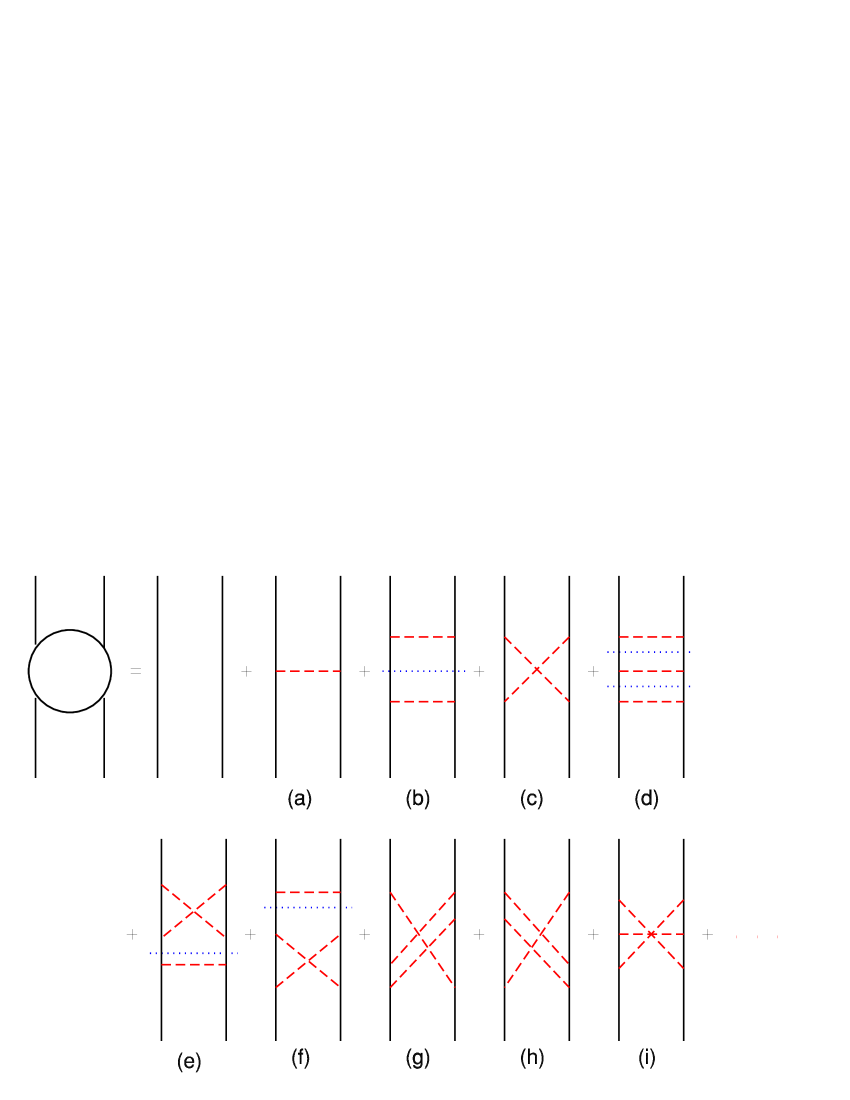
Figure 15: Feynman diagrams respresenting the two-body scattering matrix $\mathcal{M}$.

where the nucleons are represented by solid lines and the mesons are represented by the dashed lines. Note that diagrams (b), (d), (e) and (f) can be reduced to simpler diagrams by cutting across two nucleon lines as represented by the dotted lines. These diagrams are said to be two-body reducible diagrams and the remaining ones two-body irreducible diagrams. The ability to classify all of the contributing diagrams as members of one or the other of these two classes suggests that the multiple scattering series can be resummed by separating the irreducible diagrams into an interaction kernel and then using an integral equation to produce the reducible diagrams. The Feynman diagrams representing the two-nucleon irreducible kernel are shown in Fig. 16.

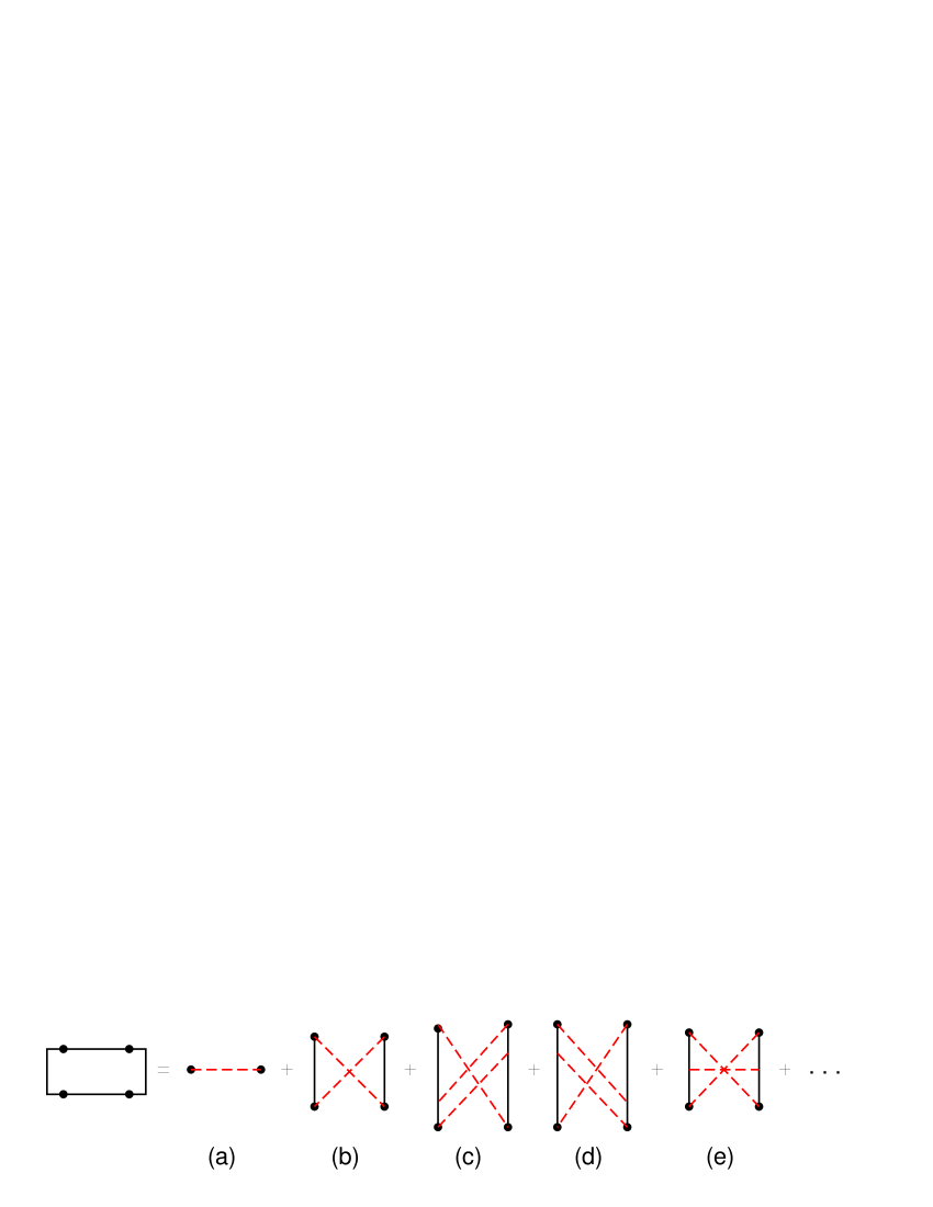
Figure 16: Feynman diagrams representing the two-nucleon irreducible kernel $V$.

The Bethe-Salpeter equation for the scattering matrix can then be written as

$$\mathcal{M}(p^{\prime},p;P)=V(p^{\prime},p,P)-i\int\frac{d^{4}k}{(2\pi)^{4}}V(p^{\prime},k;P)G_{0}(k,P)\mathcal{M}(k,p;P)$$ (52)

where $P$ is the total four-momentum of the two-body system; $p^{\prime}$, $k$ and $p$ are the final, intermediate and initial relative four-momenta of the two particles; $G_{0}$ is the free two-body propagator; and $V$ is a kernel consisting of a sum of all possible two-body irreducible diagrams. The Bethe-Salpeter equation is represented by the diagrams in Fig. 17.

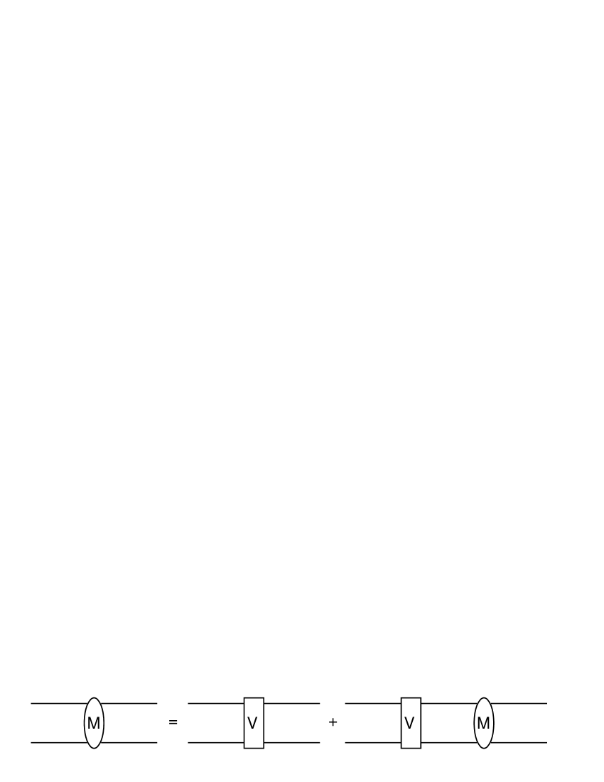
Figure 17: Diagrammatic representation of the integral equation for the scattering matrix.

Since the Feynman series is organized such that all of the individual propagators and vertices are covariant with respect to the free-particle Lorentz transformations, the sum is manifestly covariant as well. The currents can be constructed by combining the free one-nucleon currents with exchange currents obtained by attaching a photon to every possible place within the irreducible interaction kernel, as shown in Fig. 18. These currents will then satisfy the Ward-Takahashi identities [130].

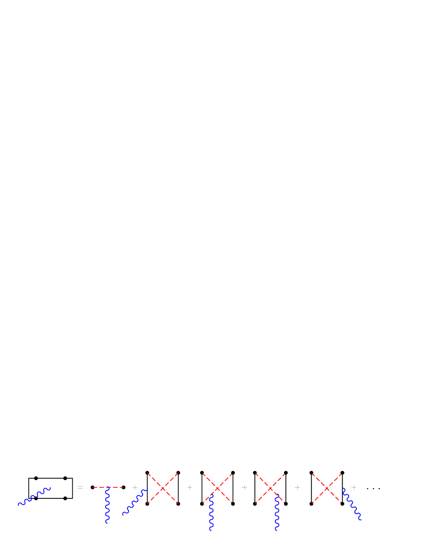
Figure 18: The two-body irreducible current diagrams.

The two-body bound state is represented by the Bethe-Salpeter vertex function $\mathcal{O}$, which satisfies

$$\mathcal{O}(p,P)=i\int\frac{d^{4}k}{(2\pi)^{4}}V(p,k;P)G_{0}(k,P)\mathcal{O}(k,P)\,.$$ (53)

This vertex function for the deuteron can be written [131] as

$$\mathcal{O}_{\lambda_{d},ba}(p,P)=\left(\Gamma(p,P)\cdot\xi_{\lambda_{d}}(P){\mathcal{C}}\right)_{ba}\,.$$ (54)

$P$ is the deuteron four-momentum, $p$ the relative momentum of the external nucleons, $\xi_{\lambda_{d}}(P)$ the polarization four-vector for the deuteron, $\mathcal{C}$ the Dirac charge conjugation matrix. The subscripts $a$ and $b$ are indices in the Dirac spinor space, and $\Gamma^{\mu}$ can be determined by basic symmetry arguments to have the general form:

$$\Gamma^{\mu}(p,P) = g_{1}(p^{2},p\cdot P)\gamma^{\mu}+g_{2}(p^{2},p\cdot P)\frac{p^{\mu}}{m}$$ (55)

$$+\frac{\!\not p_{2}-m}{m}\left(g_{3}(p^{2},p\cdot P)\gamma^{\mu}+g_{4}(p^{2},p\cdot P)\frac{p^{\mu}}{m}\right)$$

$$+\left(g_{5}(p^{2},p\cdot P)\gamma^{\mu}+g_{6}(p^{2},p\cdot P)\frac{p^{\mu}}{m}\right)\frac{\!\not p_{1}+m}{m}$$

$$+\frac{\!\not p_{2}-m}{m}\left(g_{7}(p^{2},p\cdot P)\gamma^{\mu}+g_{8}(p^{2},p\cdot P)\frac{p^{\mu}}{m}\right)\frac{\!\not p_{1}+m}{m}\,,$$

where $p_{1}=\frac{P}{2}+p$ and $p_{2}=\frac{P}{2}-p$. A generalization of the Pauli symmetry requires that

$$\Gamma^{\mu}(p,P)=-{\mathcal{C}}\Gamma^{\mu T}(-p,P){\mathcal{C}}^{-1}.$$ (56)

which places constraints on the scalar functions $g_{i}$. Note that for given values of $p$ and $P$, the vertex function depends upon eight scalar functions whereas the Schrödinger wave function of the deuteron is determined by the two functions $u$ and $w$.

The Bethe-Salpeter equation is a complete representation of all possible contributions to the two-body amplitudes for a given field theory. As such it retains all of the complexities of field theories in that there is an infinite number of contributions as represented by Feynman diagrams. The problem of particle dressing and renormalization is present, and for strong coupling theories there is no general scheme for organizing the renormalization program. As a practical matter, model calculations generally assume that all propagators represent dressed particles with physical masses. This still leaves an infinite number of contributions to the irreducible kernel. Again, there is no a priori means of establishing a reasonable truncation procedure in order to obtain a tractable set of contributions. However, the phenomenology of nuclear systems suggests that the importance of contributions to the nuclear force depends upon the range of the contributions due to the strong repulsion of nucleons at short distance. As a result, models of the deuteron using field-theoretical techniques usually assume that contributions can be ordered by range. In practice this reduces to the use of one-boson-exchange potentials. This is referred to as the ladder approximation to the Bethe-Salpeter equation.

The ladder approximation violates the crossing symmetry of the two-body scattering amplitudes, which is a property of the full Bethe-Salpeter equation. This results from the elimination of the higher-order crossed-box contributions to the kernel. A related problem is that the two-body equation no longer reduces to a one-body wave equation at the limit of infinite mass for one of the constituents (defined as the static limit) [132].

A further difficulty for producing models of the deuteron using the field-theoretical methods is that phenomenology often requires the introduction of nonrenormalizable couplings such as the derivative coupling of the pion and tensor coupling of vector mesons. The loop integration of the Bethe-Salpeter equation must then be cut off to eliminate unphysically large or infinite contributions. This is usually done by introducing form factors for strong coupling vertices, which also attempts to include finite-size effects for the hadrons. In addition, the hadrons have a finite electromagnetic size so that electromagnetic form factors are also required by the phenomenology. The introduction of form factors can, however, result in violations of gauge invariance.

The solution of the Bethe-Salpeter equation is also a calculational challenge since it is a four-dimensional integral equation with a complicated analytical structure. It has however been solved for the two-nucleon system in Euclidean space [133] and applied to the calculation of electron-deuteron scattering [134, 135].

5.6.2 Quasipotential Equations

The Bethe-Salpeter equation is a four-dimensional integral equation. As such it is much more difficult to solve numerically than the comparable nonrelativistic three-dimensional Lippmann-Schwinger equation. To simplify the solution of the relativistic equations, one resorts to the infinite class of quasipotential equations [4, 136, 137, 138, 139, 140, 141, 142, 143]. These equations are related to the Bethe-Salpeter equation (52) by replacing the free propagator $G_{0}$ by a new propagator $g$. The scattering matrix equation can now be formally rewritten as

$$\mathcal{M}(p^{\prime},p;P)=U(p^{\prime},p;P)-i\int\frac{d^{4}k}{(2\pi)^{4}}U(p^{\prime},k;P)g(k;P)\mathcal{M}(k,p;P)\,,$$ (57)

where $U$ is the quasipotential defined as

$$U(p^{\prime},p;P)\equiv V(p^{\prime},p;P)-i\int\frac{d^{4}k}{(2\pi)^{4}}V(p^{\prime},k;P)(G_{0}(k;P)-g(k;P))U(k,p;P)\;.$$ (58)

This pair of equations is equivalent to (52) and represents a re-summation of the multiple scattering series. The new propagator $g$ is usually chosen to include a constraint in the form of a delta function involving either the relative energy or time in such a way as to reduce (57) to three dimensions. In addition $g$ must be chosen such that it has the same residue as $G_{0}$ along the righthand elastic cut. This guarantees that the discontinuity of $U$ produces only inelastic contributions as in the case of (52).

Although it appears that the reduction of (57) to three dimensions is of great practical advantage, it should be noted that (58) is still a four-dimensional integral equation of difficulty comparable to (52). The real utility of these equations comes about when (58) is approximated by iteration and truncation. Then $U$ can be obtained by quadrature of (58) and used in the three-dimensional equation (57).

It would appear that we have achieved a reduction in the difficulty of solution of the problem at the expense of introducing considerable additional ambiguity since there is an infinite number of possible choices for $g$ which satisfy the above specified requirements. However, this freedom is turned to an advantage when noting that $g$ can be chosen to maximize the convergence of (58). In essence, the parts of the ladder and crossed box diagrams which tend to cancel are being summed in the quasipotential equation (58) rather than in the equation for the scattering matrix (57). Indeed, the lowest order calculations using a variety of quasipotential prescriptions have been calculated for scalar particles [144] and shown to be closer to the results of the complete Bethe-Salpeter equation than is the result from the ladder approximation to the Bethe-Salpeter equation. In addition, it has been shown that there exists an infinite number of quasipotential equations which have the correct static limit. This is also a reflection of the improved convergence of these quasipotential equations [145].

The results from three different quasipotential models are presented here. The first of these is the calculation of Hummel and Tjon (HT) [146] based on the BSLT equation [136]. In this case, the propagator $g_{BSLT}$ contains a term $\delta(p_{0})$ which forces the relative energy of the two nucleons to zero. One can say that the two nucleons are equally off mass-shell. The vertex functions are calculated using the BSLT equation with a one-boson exchange interaction. They still have eight components. The current matrix elements are then calculated by replacing the Bethe-Salpeter vertex functions with the BSLT vertex function, assuming that it is energy independent. In the examples shown here the nucleon electromagnetic form factors are taken to be the Höhler 8.2 parameterization.

The second model is that of Phillips, Wallace and Devine (PWD) [147, 148, 149] where a one-boson-exchange interaction is used with the single-time equation that introduces a constraint that the relative time be zero. This is very close to the HT approach since this choice means that the propagator $g_{ET}$ is independent of the relative energy of the two nucleons. The single-time deuteron vertex functions still have eight components. A consistent treatment of the current is constructed to guarantee current conservation, but Lorentz covariance is violated. The MMD parameterization of the nucleon electromagnetic form factor are used.

The third model is that of Van Orden, Devine and Gross (VODG) [150, 151, 152], based on the Gross equation [141, 142]. One of the nucleons is placed on its positive energy mass shell, which gives:

$$g_{Gross}\propto\frac{1}{p_{2}^{2}-m^{2}+i\varepsilon}\delta^{(+)}(p_{1}^{2}-m^{2})$$ (59)

Since this constraint is itself manifestly covariant, the Gross equation amplitudes are manifestly covariant. But it is not symmetric in the nucleons and the exchange symmetry must be recovered by symmetrizing the interaction kernel. This procedure introduces unphysical singularities, which are treated in principal value to avoid unitarity problems and have little numerical effect in a weakly bound system such as the deuteron. As a result of placing one nucleon on shell in (55), the Gross equation deuteron vertex function has four-components that can be represented in terms of an $S$ wave, a $D$ wave and singlet and triplet $P$ wave functions.

A systematic procedure for constructing the effective current operators for the Gross equation exists [153] and has been shown to be rigorous to all orders and remarkably robust under trucation [154]. The result is that Ward identities for the Gross equation are maintained and the calculation is gauge invariant.

A one-boson-exchange interaction is used, that has been fit to $NN$ scattering data up to a lab kinetic energy of about 300 MeV [155, 156]. The fit is reasonable, but not at the level of precision obtained with modern fully phenomenological potentials.

Several unique features appear in this model. All of the strong vertices are multiplied by a product of three form factors,

$$h(p^{\prime 2})h(p^{2})f((p^{\prime}-p)^{2})\,.$$ (60)

Here $p$ and $p^{\prime}$ are the initial and final four-momenta of the nucleon and $p^{\prime}-p$ is the four-momentum of the meson. The meson form factor is taken to be

$$f(\ell^{2})=\frac{(\Lambda_{\mu}^{2}-\mu^{2})^{2}+\Lambda_{\mu}^{4}}{(\Lambda_{\mu}^{2}-\ell^{2})^{2}+\Lambda_{\mu}^{4}}$$ (61)

and the nucleon form factor

$$h(p^{2})=\frac{2(\Lambda_{n}^{2}-m^{2})^{2}}{(\Lambda_{n}^{2}-p^{2})^{2}+(\Lambda_{n}^{2}-m^{2})^{2}}\,.$$ (62)

The prescription of Gross and Riska [153] is used to construct a single-nucleon electromagnetic current which is consistent with the strong-vertex form factors and phenomenological single-nucleon electromagnetic form factors. This current is constructed in such a manner that the one- and two-body Ward identities are of the same form as for the local field theory. The simplest form that this single-nucleon current can take is

$$J^{(i)\mu}(p^{\prime},p) = F_{1}(Q^{2})f_{0}(p^{\prime 2},p^{2})\,\gamma^{\mu}+\frac{F_{2}(Q^{2})}{2m}h_{0}(p^{\prime 2},p^{2})\,i\sigma^{\mu\nu}q_{\nu}$$ (63)

$$\quad+F_{10}(Q^{2})g_{0}(p^{\prime 2},p^{2})\,\frac{\!\not p^{\prime}-m}{2m}\,\gamma^{\mu}\,\frac{\!\not p-m}{2m}\,,$$

where the nucleon form factors are

$$F_{i}(Q^{2})=\frac{1}{2}\left(F_{i}^{S}(Q^{2})+F_{i}^{V}(Q^{2})\cdot\tau_{3}\right)\,.$$ (64)

The factors that depend upon the nucleon momenta are

$$f_{0}(p^{\prime 2},p^{2})\equiv\frac{h(p^{2})}{h(p^{\prime 2})}\,\frac{m^{2}-p^{\prime 2}}{p^{2}-p^{\prime 2}}+\frac{h(p^{\prime 2})}{h(p^{2})}\,\frac{m^{2}-p^{2}}{p^{\prime 2}-p^{2}},$$ (65)

and

$$g_{0}(p^{\prime 2},p^{2})\equiv\left(\frac{h(p^{2})}{h(p^{\prime 2})}-\frac{h(p^{\prime 2})}{h(p^{2})}\right)\frac{4m^{2}}{p^{\prime 2}-p^{2}}\,.$$ (66)

The function $h_{0}(p^{\prime 2},p^{2})$ must be equal to one when both nucleons are on mass shell, but is otherwise unconstrained. For simplicity, the calculations shown here use $h_{0}=f_{0}$. The form factor $F_{10}(Q^{2})$ must obey $F_{10}(0)=1$, but is otherwise unconstrained and is chosen to be of a dipole form.

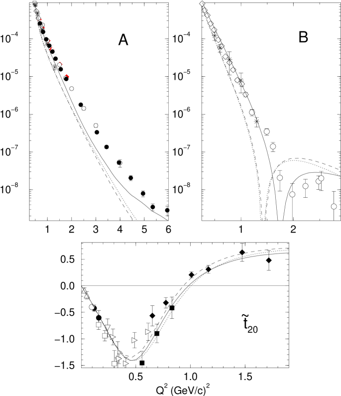
Figure 19: Elastic $ed$ scattering observables calculated with Quasipotential equations. HT-RIA, NEMFF: H (dotted curve); PDW-RIA, NEMFF: MMD (dashed); VODG-CIA, NEMFF: MMD (solid).

Figure 19 shows the elastic structure functions for these models calculated in the relativistic impulse approximation (RIA). As expected from the nature of the quasipotential approximations, the calculations of HT and PWD lead to very similar results for all three observables (in spite of the fact that they use different NEMFF). The VODG calculation uses the MMD form factors. For $A(Q^{2})$, it is systematically larger than the others due to additional contributions that are necessary to conserve the current within the context of the Gross equation. These additions yield to the so-called Complete Impulse Approximation (CIA).

For $B(Q^{2})$, the HT and PWD calculations are systematically below the data and have a minimum at a lower $Q^{2}$ than is indicated by the data. The VODG calculation is higher and has a minimum at higher $Q^{2}$ than the other two calculations. This difference has been shown to be due to a small $P$ wave component of relativistic origin that contributes to the normalization of the vertex function at the level of 0.01% [152]. This clearly indicates the sensitivity of the position of the $G_{M}$ node to small components.

Finally, in the case of $\tilde{t}_{20}(Q^{2})$, the three models have a very similar behavior.

The sensitivity of the observables to the choice of single-nucleon form factors is shown in Fig. 20, using the VODG calculation in the CIA approximation. All but the VO2 parameterization are standard form factors that appear in the literature. The VO2 form factor is modeled after the MMD form factor but adjusted to fit the new data on $G_{E}^{p}/G_{M}^{p}$ from Jefferson Lab [157]. As expected from the discussion in App. C, $A(Q^{2})$ and $B(Q^{2})$ are very sensitive to the choice of single nucleon form factor while $\tilde{t}_{20}(Q^{2})$ is almost totally insensitive to it. The various $A(Q^{2})$ curves in Fig. 20 may be directly related to the corresponding $G_{E}^{S}$ curves in Fig. 33. Note that for the relativistic approaches, in contrast to the NRIA, the nucleon form factors cannot simply be factorized, so that there is no reason that $\tilde{t}_{20}(Q^{2})$ be completely independent of the NEMFF. Much more accurate data on the single-nucleon form factors that will be forthcoming from experimental facilities around the world will, hopefully, provide much greater constraints on these form factors.

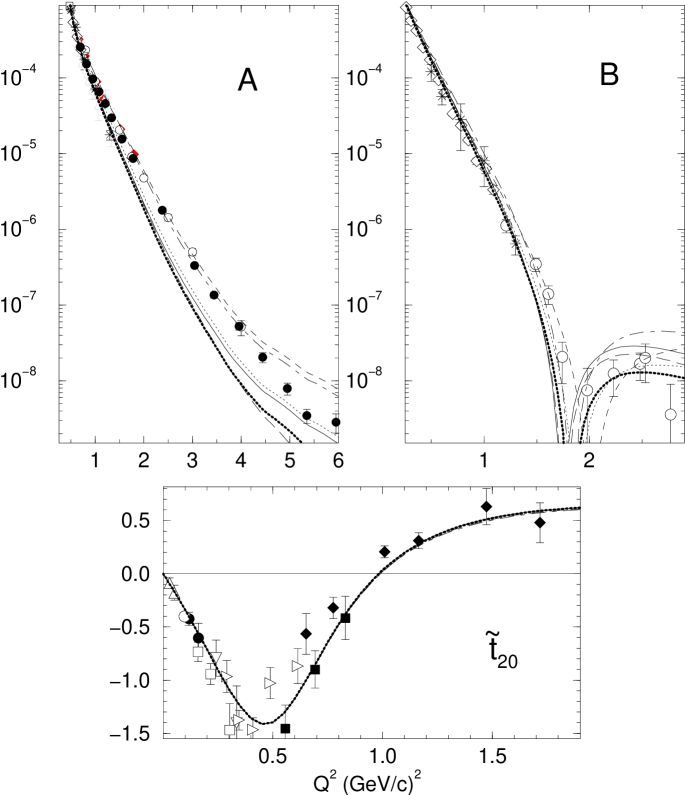
Figure 20: Deuteron elastic structure functions calculated using the CIA of VODG with various parameterizations of the nucleon form factors: Galster (dotted curve), Höhler (long dashed), GK85 (dot-dashed), GK92 (dashed), MMD (solid), VO2 (thick dotted).

Figure 21 shows the effect of the addition of $\rho\pi\gamma$ exchange currents to the three calculations. HT were the first to implement the calculation of the $\rho\pi\gamma$ contribution to the deuteron form factors in a relativistic model. They also included a $\omega\sigma\gamma$ exchange current, which compensates their large effect of the $\rho\pi\gamma$. This last contribution is not present in the calculation presented here, because there is considerable uncertainty about the $\sigma$ meson, and consequently about its couplings and vertex form factors (see [158] for a recent discussion of the $g_{\omega\sigma\gamma}$ coupling constant). Two sets of calculations for the VODG structure functions are shown, one with the MMD form factors as before, and one with the VO2 form factors. Comparing to Fig. 19, it is clear that this exchange current can result in considerable variation in $A(Q^{2})$. The variation in $B(Q^{2})$ is much smaller, in part because of the smaller $Q^{2}$ range considered. The $\rho\pi\gamma$ exchange current shifts the node of $G_{M}$ to lower values of $Q^{2}$ for all calculations, in contrast with the nonrelativistic calculations using the $v/c$ expansion where this current has the opposite effect. This is the result of the tensor coupling of the $\rho$ to the nucleon, which appears to be a higher order contribution in the $v/c$ expansion, but weighted by a large coefficient. In this way, expansion schemes may lead to wrong estimates without a careful examination of higher-order contributions. Finally, the addition of the $\rho\pi\gamma$ contribution has a small effect on $\tilde{t}_{20}(Q^{2})$, but brings the calculations in a somewhat better agreement with the available data.

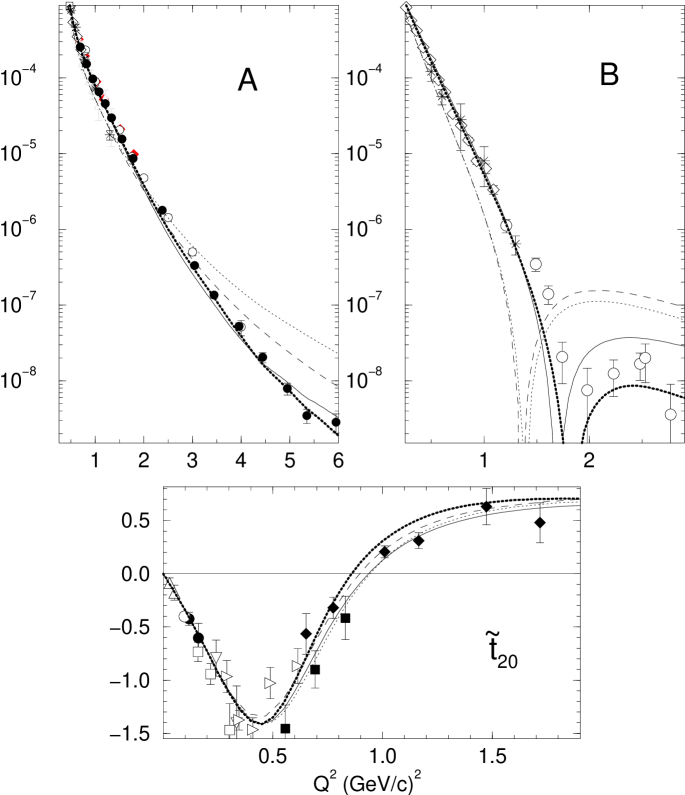
Figure 21: Elastic $ed$ scattering observables calculated with Quasipotential equations, including the $\rho\pi\gamma$ contribution. HT (dotted curve), PDW (dashed), VODG-MMD (solid), VODG-SO2 with $F_{10}$ off-shell form factor adjusted (thick dotted).

The variation in the $\rho\pi\gamma$ contributions from the various models [146, 159, 160, 161] is associated with ambiguities in these contributions. Although the coupling constant for the $\rho\pi\gamma$ vertex is constrained by the decay width $\Gamma(\rho\rightarrow\pi\gamma)$, little is known about the fall off of the associated form factor. Figure 22 shows a number of different form factors for this vertex. HT use the VMD form factor which is the hardest of the available form factors while VODG use the Rome 2 form factor which is the softest one. PWD use an intermediate parameterization. The $A(Q^{2})$ data favor the use of the softest possible form factor. In contradistinction, a recent theoretical reexamination of the $\rho\pi\gamma$ form factor [162] results in a dependence close to the VMD one. Whether the $\rho\pi\gamma$ contribution to the deuteron form factors is really small, or suppressed by other contributions is still an open question.

Figure 22: Different prescriptions for the $\rho\pi\gamma$ form factor: VMD (dotted curve), Gross-Ito [159] (dashed), Rome 1 [160] (long dashed), Mitchell-Tandy [161] (dot-dashed), Rome 2 [160] (solid).

Another source of ambiguity, explicitly present in the the VODG calculation, is the choice of the form factor $F_{10}(Q^{2})$ in (63). In these calculations, $F_{10}(Q^{2})$ is adjusted to optimize the fit of the calculation to the data for the deuteron structure functions. By using a very hard form factor it is possible to obtain an extremely good fit to the data. This along with ambiguities in the $\rho\pi\gamma$ form factor means that no absolute predictions of the structure functions can be obtained unless some means can be found to physically constrain the ambiguities in the models.

5.6.3 Light-front field theory

The above approaches based on the Bethe-Salpeter equation are generally discussed in the context of Feynman perturbation theory with equal time quantization. Microcausality, however, only requires that the theory be quantized on a spacelike hypersurface. A special limiting case of such a surface is the light cone where the spacetime interval approaches zero. Quantizing field theories on the light cone has long been common practice in describing deep inelastic scattering where the large four-momenta kinematically favor contributions to scattering very near the light cone. Typically, the light-cone approach is organized as a “time-ordered” perturbation expansion in terms of the light-front time $x^{-}=x^{0}-x^{3}$. The wave functions are then Fock-space wave functions with a probabilistic interpretation as in the case of Schrödinger wave functions.

A particular problem with light-front field theory is that the conventional choice of a fixed light-front orientation violates manifest covariance, although matrix elements remain covariant. One solution to this problem [163] is to describe the quantization surface in terms of an arbitrary direction on the light cone given by a light-like four-vector $\omega^{\mu}$ and require that the quantization surface be described by $\omega\cdot x=0$. This renders the theory manifestly covariant, at the expense of the additional complication that the wave functions and operators become dependent on the vector $\omega$. This is covariant light-front dynamics (LFD). Matrix elements and observables, in a complete calculation, do not depend on $\omega$. In a practical calculation, a definite procedure to eliminate the non physical $\omega$-dependent terms is applied.

The deuteron elastic structure functions from this approach [163, 164, 165] are shown in Fig. 23.

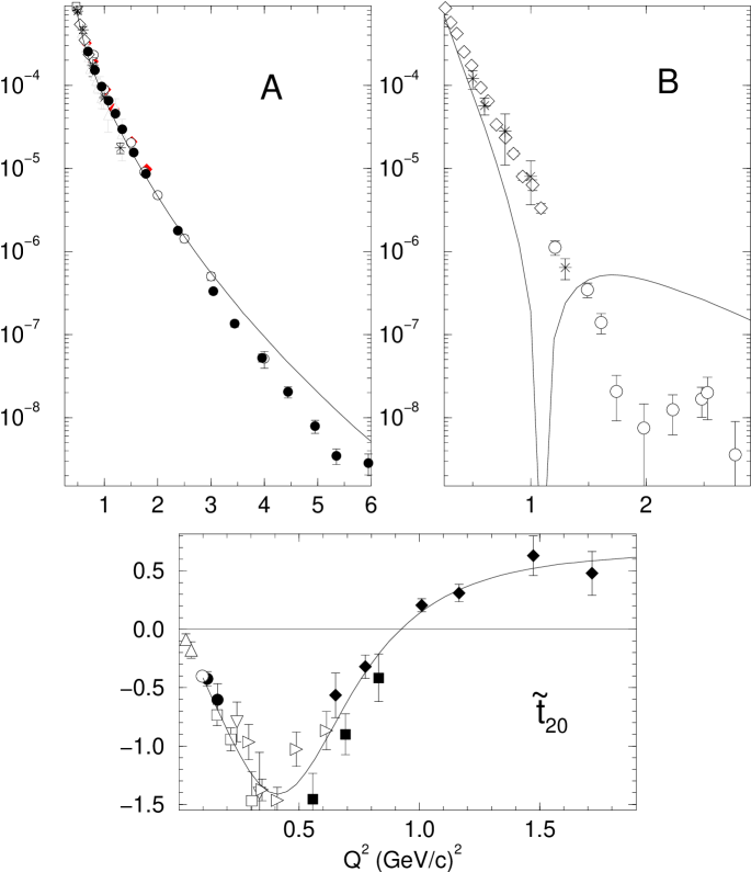
Figure 23: Elastic $ed$ scattering observables calculated within light-front dynamics.

In these calculations, the deuteron wave function has six components ($f_{i}$), two of which ($f_{1}$ and $f_{2}$) correspond to the usual $S$ and $D$ components in the nonrelativistic limit. These components are calculated perturbatively from the usual nonrelativistic wave function. Schematically [166],

$$\psi(\mathbf{k},\mathbf{n};f_{1},f_{2},f_{3},f_{4},f_{5},f_{6})\sim\int V(\mathbf{k^{\prime}},\mathbf{k},\mathbf{n},M_{d})\psi_{NR}(\mathbf{k};u,w)d^{3}\mathbf{k^{\prime}}\,,$$ (67)

where $\mathbf{k}$ is the relative momentum of the two nucleons and $\mathbf{n}$ a unit vector along the three-vector $\omega$. The $NN$ interaction kernel $V$ is of a one-boson-exchange type, calculated within the framework of LFD using the parameters (such as coupling constants) of the Bonn potential. The single-nucleon electromagnetic form factors are the MMD parameterization (the effect of various NEMFF was considered in [165]). This calculation produces a reasonable description of the data for $A(Q^{2})$ and $\tilde{t}_{20}(Q^{2})$ but the minimum in $B(Q^{2})$ occurs well below the position indicated by the data. Given the sensitivity of the magnetic form factor to small effects, this may simply be the result of the perturbative treatment of the small components of the wave functions in this calculation.

Indeed, work is in progress to improve the calculation of the interaction kernel $V$ and of the complete wave function [167]. Meson exchange contributions are only partially included in the original calculations. The addition of recoil terms and of the $\rho\pi\gamma$ contribution was also initiated: the recoil terms move the node of $G_{M}$ to higher $Q^{2}$, while the $\rho\pi\gamma$ contribution does not modify appreciably any observable up to $Q^{2}\sim 2$ (GeV/c)² [168]. A complete calculation using LFD seems at hand and very promising.

5.6.4 Effective field theory

In principle, all these field theoretical techniques should yield the same results, given the same dynamical input. This statement applies to the calculated matrix elements which are the physical observables of the field theory. The identification of wave functions and operators varies from formulation to formulation and do not have unique meanings. Furthermore, within any given formulation, unitary transformations of the Lagrangian, such as field redefinitions, can also move contributions between the wave functions and operators. Such ambiguities are already present in nonrelativistic models, which may be shown to be equivalent, at least in part, up to a unitary transformation [44, 169]. None of this would be of particular concern if it were not necessary to truncate all of the approaches for reasons of practicality. Consequently, the physical content of the various formulations varies, resulting in a variety of ambiguities, some of which have been discussed above. A major problem then is that there is, in general, no organizing principle present in these calculations which indicates the relative importance of various physical contributions to guide the choice of truncation schemes.

A promising development that could help to resolve this problem is the application of effective field theories to nuclear systems [170, 171, 172, 173, 174, 175, 176, 177, 178]. The basic idea of effective field theory is that at low energies the observables of a theory are largely insensitive to the details of short-range contributions to the interactions. The long-range degrees of freedom are then treated in detail and the short range pieces are replaced by contact interactions. The Lagrangian is written as a sum of terms containing contact interactions with increasing numbers of derivatives of the fields. This constitutes an expansion of the theory in terms of momenta which are small compared to some scale chosen to separate the short and long range physics. Contributions to observables are then ordered according to this small momentum, providing a well defined counting scheme that controls approximations to the theory.

For nuclear systems, the appropriate effective field theory is Chiral Perturbation Theory ($\chi$PT) since the long-range part of the nuclear force is associated with the pion, a Goldstone boson. A considerable amount of effort is being expended in the application of $\chi$PT to low energy nucleon-nucleon scattering and to the deuteron. The $NN$ system is particularly challenging in that its scattering lengths are large, although its bound state, the deuteron, is only weakly bound. This implies that there is a dynamical scale in the problem in addition to the chiral scale. The application of $\chi$PT to the deuteron has followed two approaches. The first [170] applies the chiral counting scheme at the level of the interaction kernel. This approach appears to converge, but is cutoff dependent at each order. The second [173, 174] applies the counting scheme at the level of the scattering matrix and current matrix elements and treats the pions perturbatively while iterating the contact interactions. It gives results that are cutoff independent, but does not appear to be converging [179]. The problem of maintaining a consistent counting scheme in the infinite sums of diagrams necessary to describe the bound states has not yet been resolved. From the standpoint of the various models used at higher momentum transfers, it is to be hoped that effective field theory will provide some insight into the organization of the various approaches.

5.7 Deuteron models with nucleon isobar contributions

In all of the approaches and models discussed to this point, the assumption has been made that the only relevant degrees of freedom are the nucleons and mesons. However, excitations of the nucleons to isobar states may produce contributions to the interactions of the same range as the heavier mesons. The deuteron wave function is in this case modified to include, in addition to the $S$ and $D$ wave $NN$ components, $\Delta\Delta$ and $NN^{*}$components. A neutrino experiment, though subject to interpretation, indicates an upper limit of 0.4 % to the amount of $\Delta\Delta$ components in the deuteron [180].

Examples of two calculations including these additional isobaric components are shown here. In both cases, the basic model involves interactions due to one meson exchange which can couple the nucleon-nucleon channel with channels containing isobars. The quark model is used to relate isobar-meson couplings (for instance $\Delta\Delta\pi$) to the corresponding nucleon-meson couplings. The fully coupled (nonrelativistic) system is then solved for the deuteron bound state and the nucleon-nucleon scattering states. Figure 24 shows the calculations of Dymarz and Khanna (DK) [181] and Blunden et al. (BGL) [182]. In both cases presented here, only the $\Delta(1232)$ isobar is included, and the $\Delta$ electromagnetic form factors are assumed to be proportional to the NEMFF. The DK calculation contains $\Delta\Delta$ components ${}^{3}S_{1},^{3}D_{1},^{7}D_{1},^{7}G_{1}$ with a total probability of $0.36\%$. The elastic form factors include contributions from single-nucleon currents with the GK form factors, nucleon pair and $\rho\pi\gamma$ exchange currents and the isobar current contributions. Two models are shown for BGL, both with only ${}^{3}D_{1}$ and ${}^{7}D_{1}$ $\Delta\Delta$ components.. Two different quark models are assumed to fix at a given radius $r_{0}$ the boundary conditions used in the determination of the wave functions. Model C’ has $r_{0}=0.74$ fm and yields an isobar contribution of $1.8\%$, while model D’ uses the Cloudy Bag Model to fix $r_{0}$ at 1.05 fm and results in an isobar contribution of $7.2\%$. Meson exchange contributions are included as well.

Within these models, $\tilde{t}_{20}$ is very sensitive to the amount of $\Delta\Delta$ components and favors the smallest probability. Although the BGL model C’ with the Höhler NEMFF seems to give an adequate description of the data, there is considerable ambiguity in these calculations due to a lack of knowledge of the isobar magnetic moments and form factors along with the difficulty of completely constraining the isobar contributions from the $NN$ scattering data. It is clear, however, that isobar components must ultimately be considered in any complete calculation of deuteron electromagnetic properties in the context of hadronic models.

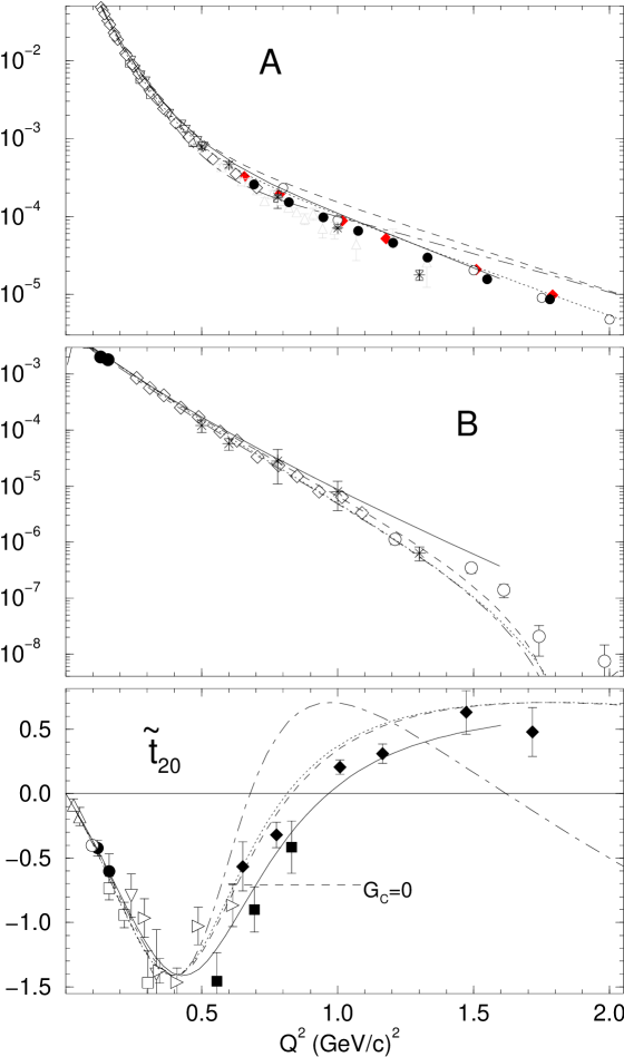
Figure 24: Elastic $ed$ scattering observables for models including nucleon isobar components. DK, NEMFF: GK [181] (solid curve); BGL-C’, NEMFF: H [182] (dotted); BGL-C’, NEMFF: GK (dashed); BGL-D’, NEMFF: GK (dot-dashed).

5.8 Quarks and gluons

5.8.1 Nonrelativistic quark models

Ultimately, many of the ambiguities associated with the hadronic model calculations can only be removed by describing the deuteron in terms of the fundamental quark and gluon degrees of freedom. In the absence of the capability to directly solve the QCD Lagrangian at low energies for the deuteron, we are left to explore possible QCD effects in the context of quark models. This greatly increases the difficulty of treating the $NN$ system since what is a two-body problem in the hadronic models, becomes at least a six-body problem for quark models. Calculations for two examples of quark cluster models are presented here. These calculations are very similar in concept and are based on a quark cluster model using the resonating group method to describe the interaction of the two three-quark clusters. The quarks interact via a quadratic confining potential and a one-gluon-exchange potential. Long range interactions are also provided via $\pi$ and $\rho$ exchange between quarks. The calculation of Buchmann, Yamauchi and Faessler (BYF) [183] contains only the $\pi$ exchange interaction, while that of Ito and Kisslinger (IK) [184] contains both meson-exchange contributions. This approach naturally contains currents associated with the individual clusters as well as exchange currents associated with quark exchange between clusters. Since the cluster wave functions are derived using oscillator-like confining forces, the cluster form factors tend to have a Gaussian form. This is clearly not consistent with the data for single-nucleon form factors and in both cases the electromagnetic cluster form factors are replaced by phenomenological NEMFF. The results are shown in Fig. 25. Neither of these calculations provides an adequate description of the data, but given their necessary simplicity, they are remarkably close to the data. In the BYF calculation, the impulse approximation is not as reliable as in $NN$ models because of the simple modeling of the intermediate range interaction, but the size of the genuine quark exchange contributions, due to the antisymmetrization of the six-quarks wave function, is significant enough to affect a comparison with the data.

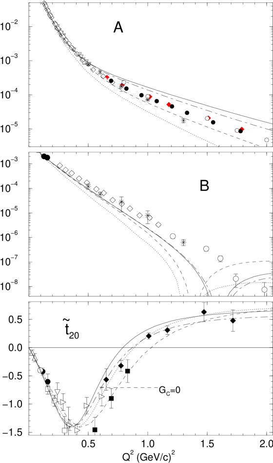
Figure 25: Elastic $ed$ observables calculated with quark-cluster models. IK [184] (dotted curve); BYF [183]: IA (dashed); BYF: IA + MEC (dot-dashed); BYF: former + quark exchange contributions (solid).

5.8.2 Perturbative QCD

This subject was reviewed recently [12]. The success and shortcoming of perturbative quantum-chromodynamics (PQCD) applied to the asymptotic behaviour of form factors may be better illustrated now with recent data from Jefferson Lab. We will only recall briefly the main predictions:

• Dimensional scaling [185]: this property can be derived within QCD, but is more general and was established before this theory. It is based on the hypothesis that the momentum transfer is shared among all the constituent quarks of the system. In the case of a hadron composed of $n$ quarks, one would expect the leading form factor to behave asymptotically as $Q^{-2(n-1)}$. Qualitatively, this can be viewed as the probability of having $n-1$ quarks within a transverse distance of $1/Q$ of the quark struck by the virtual photon. Since this must be true both in the initial and final states, one expects $F^{2}\sim Q^{-4(n-1)}$ and for the deuteron ($n=6$), $A\sim Q^{-20}$.

• Logarithmic corrections to the leading amplitude, together with the factorization of the nucleon form factors in the weak binding limit, yield [186]:

  $$\sqrt{A}\sim F_{N}^{2}\left(\frac{Q^{2}}{4}\right)\cdot\frac{1}{Q^{2}}\cdot\left(\ln\frac{Q^{2}}{\Lambda^{2}}\right)^{-1+\epsilon}$$ (68)

  where $F_{N}$ is the nucleon form factor, $\Lambda$ an energy scale characteristic of QCD ($\Lambda\simeq 200$ MeV) and $\epsilon$ a calculable number much smaller than 1. An attempt to directly compute $A$ and its normalization in PQCD was not successfull [12, 187].

• Helicity conservation at each photon/gluon-quark vertex implies that the dominant contribution to elastic electron deuteron scattering should come from the configuration where the deuteron has helicity zero in both initial and final states [188]. Expressing the form factors in an helicity basis in the light-cone frame, this is equivalent to the prediction that $G_{00}^{+}$, the “$+$” component of the current matrix element between states of helicity $0$, is the leading amplitude. It was argued [189] that this helicity conserving amplitude should dominate the $ed$ scattering for $Q^{2}\gg 2\Lambda m_{d}\simeq 0.8$ (GeV/c)². Other components $G_{+0}^{+}$ (single helicity flip) and $G_{+-}^{+}$ (double helicity flip) should be suppressed by respectively one and two powers of $Q$:

  $$G_{+0}^{+}=a\left(\frac{\Lambda}{Q}\right)G_{00}^{+}\quad\hbox{and}\quad G_{+-}^{+}=b\left(\frac{\Lambda}{Q}\right)^{2}G_{00}^{+}\quad\hbox{when}\;Q\rightarrow\infty$$ (69)

  Since the usual form factors are linear combinations of the $G_{hh^{\prime}}^{+}$’s, the asymptotic behaviour of observable ratios such as $B/A$, $t_{20}$ and $t_{21}$ can easily be calculated. Note that the logarithmic corrections such as appearing in (68) may only be calculated for the dominant, helicity conserving, form factor. Equation (69) thus assumes the same logarithmic corrections for all helicity amplitudes.

How do these predictions compare with recent $ed$ data ? The $A$ data, now extending up to $Q^{2}=6$ (GeV/c)² [98], is suggestive of the expected $Q^{-20}$ behaviour, though a $Q^{-16}$ behaviour is still not excluded (see Fig. 26): a fit using the five highest $Q^{2}$ data points in Ref. [98] to the dependence $A\sim Q^{-2m}$ yields $m=8.0\pm 0.6$. Excluding the less precise last point yields $m=8.7\pm 0.7$. More interestingly, using the dipole form factor for $F_{N}$ in (68), the $Q^{2}$ behaviour of $A$ is reproduced between 2 and 6 (GeV/c)². As for the helicity amplitudes, their behaviour is tested only up to $Q^{2}\simeq 2$ (GeV/c)², which is the range of the available $B$ [96] and $t_{2j}$ [103] data. The pure dominance of the helicity $0\rightarrow 0$ transition ($a=b=0$ in (69) [189]) does not account for this data (see Fig. 27). The prescription $a=5$ and $b=0$ [190] was built to generate a node in $G_{M}$, but in order to qualitatively reproduce the $t_{2j}$ data as well, one is led to $a=1.8$ and $b=38$ [191]. This implies that the double helicity flip amplitude is as large as the non helicity flip amplitude and contradicts the applicability of PQCD in the momentum range considered. Fits to data using these helicity amplitudes lead to the same conclusion [78, 192]. All these simple ansatz lead to a sharp increase of the ratio $B/A$ for $Q^{2}\geq 2.5$ (GeV/c)², which may be an interesting feature for planned experiments at JLab.

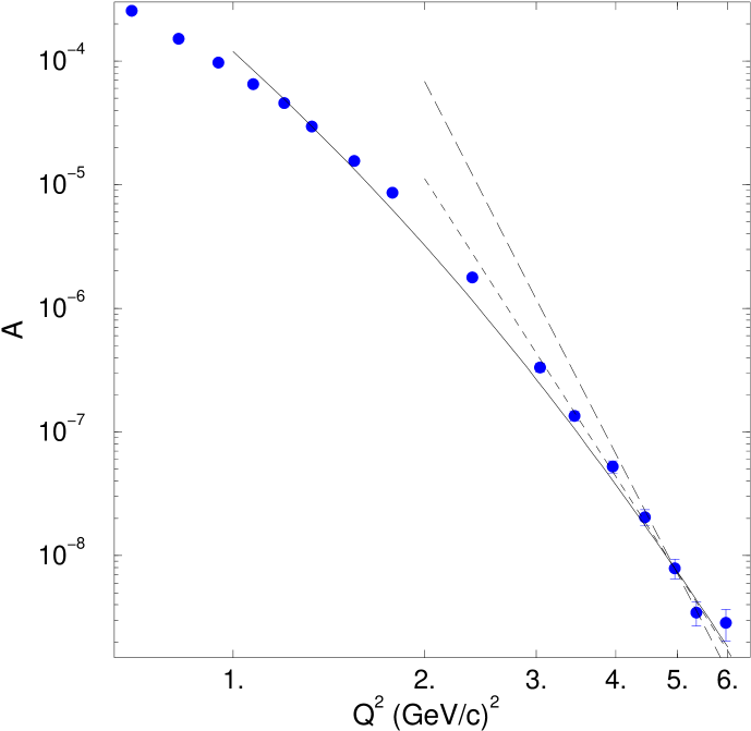
Figure 26: $A(Q^{2})$ in a Log-Log scale. The data is from JLab/HallA [98]. The straight lines illustrate a $Q^{-16}$ (dashed) and a $Q^{-20}$ (long-dashed) dependence. The solid line represents Eq.(68). All curves are normalized to the point at $Q^{2}=4.95$ (GeV/c)².

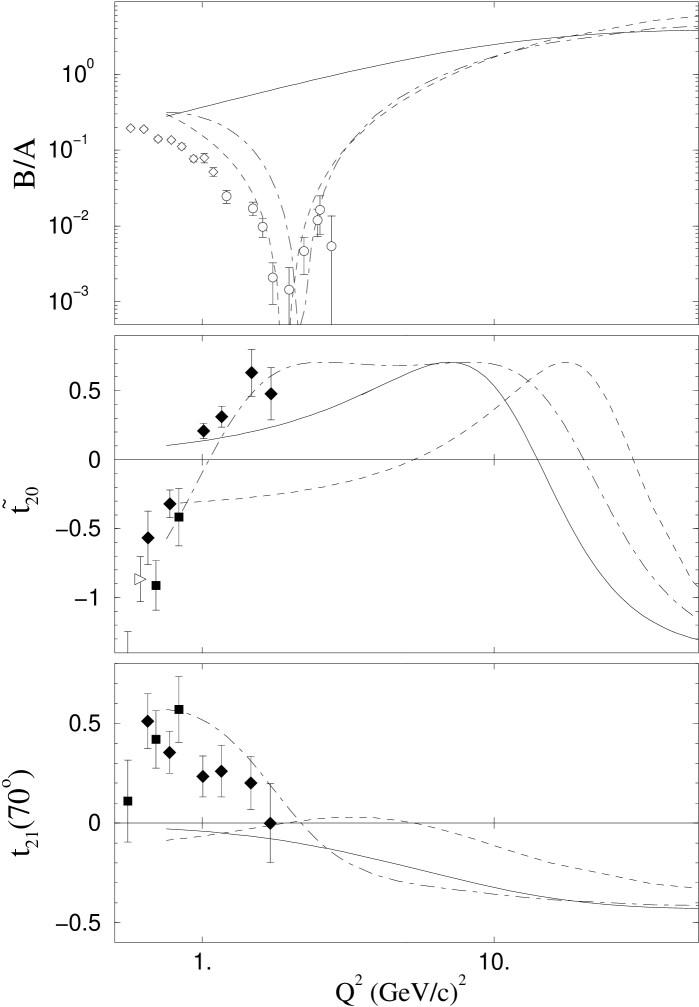
Figure 27: Ratios $B/A$, $\widetilde{t}_{20}$ and $t_{21}$ from light-cone frame helicity amplitudes. The curves correspond to Eq.(69) with different values of $a$ and $b$ (see text), from Refs. [189] (solid line), [190] (dashed) and [191] (dot-dashed). Note the logarithmic scale in $Q^{2}$.

5.9 Further comparison between models and data

To conclude this section, we recapitulate some of the theoretical results, in comparison with observables (Fig. 28) and data on separated form factors (Fig. 29). In the case of $A$ and $B$, deviations with respect to an average representation of the data (parameterization I) are presented. A summary of remaining ambiguities and foreseable progress will be given in Sec. 8.

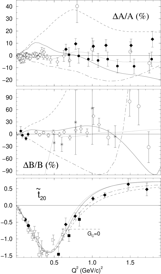
Figure 28: $\Delta A/A$ and $\Delta B/B$, in %, and $\tilde{t}_{20}$ as a function of $Q^{2}$. The deviations of $A$ and $B$ are calculated with respect to parameterization I. $A$ data legend: Saclay [97] (open diamonds), SLAC [90] (open circles), JLab/HallA [98] (filled circles), JLab/HallC [99] (filled diamonds). $B$ data legend: see Fig. 8. $\tilde{t}_{20}$ data legend: see Figs. 6 and 8. Theoretical calculations: NRIA + MEC + relativistic corrections (Sec. 5.4) [123] (dashed curve) and [42] (dotted), CIA + MEC (Sec. 5.6.2) updated from [151] (solid), LFD (Sec. 5.6.3) [165] (dot-dashed).

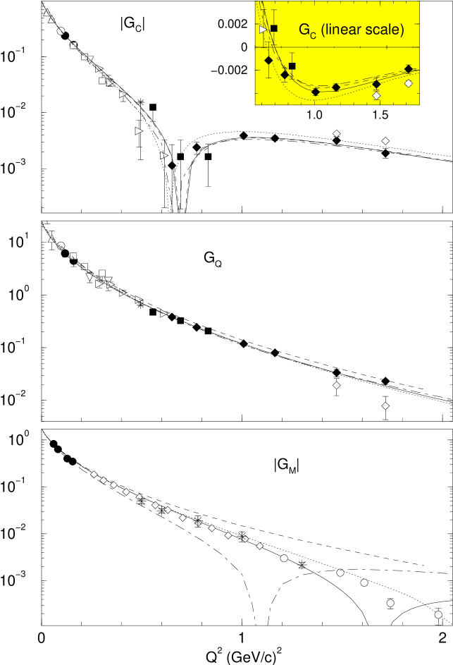
Figure 29: Deuteron form factors $G_{C}$, $G_{Q}$ and $G_{M}$ as a function of $Q^{2}$. Same legend as Fig. 28.

6 The nucleon momentum distribution in the deuteron

Several processes have been investigated for which the cross sections, in the nonrelativistic impulse approximation, are proportional to the distribution of the internal momentum $p$ in the deuteron,

$$\rho(p)=u^{2}(p)+w^{2}(p)\,,$$ (70)

with $u(p)$ and $w(p)$ defined by Eq.(8). Note that $\mathbf{p}$, the conjugate variable of the relative coordinate $\mathbf{r}$, is half the relative momentum between the two nucleons, so that an experiment probing a momentum $p$ may be related to elastic electron scattering at a momentum transfer $q=2p$. These processes include quasi-free scattering on one of the nucleons, $d(p,2p)n$, $d(e,e^{\prime}p)n$ and $d(e,e^{\prime})$, or equivalently the detection of the spectator proton in high energy deuteron hadronic break-up, $A(d,p)$ . Indeed, they all are proportional to $\rho(p)$ up to $p\simeq 200$ MeV/c , but deviations from the impulse approximation occur for higher values of $p$ . Final state interaction, dynamical excitation of the $\Delta$ resonance and in inclusive reactions pion production have then to be taken account, thus rendering the interpretation of the experiments less straightforward.

Another interesting feature of these processes is the possibility to access the ratio $w(p)/u(p)$ with the measurement of deuteron tensor polarization observables. A simple relationship between the analyzing power $T_{20}$ and the ratio $w(p)/u(p)$ can be derived in the (nonrelativistic) impulse approximation, and again deviations are seen, or are to be expected, above $p\simeq 200$ MeV/c .

6.1 d(e,e’p)n measurements at high missing momenta

The study of the single-particle properties of nuclei through $(e,e^{\prime}p)$ reactions are the subject of an excellent review [7]. Concerning the deuteron, the (neutron) missing momentum is identified, in the plane-wave impulse approximation (PWIA), with the internal momentum $p$ . The experiments reaching the highest missing momenta have been carried out at Saclay (500 MeV/c) [193], NIKHEF (700 MeV/c) [194] and MAMI (950 MeV/c) [195], but in kinematical conditions which are not always optimal to study the high momentum components in the deuteron wave function. Deviations from the PWIA are of the order of 50 % at 500 MeV/c and can reach a factor 10 at 1 GeV/c (see Fig. 30). They can be understood, if only qualitatively at the highest missing momenta, in terms of final state interactions, meson exchange currents and $\Delta$ excitation.

Figure 30: Ratio of the experimental $d(e,e^{\prime}p)n$ to the calculated PWIA (using the Paris potential) cross sections, corresponding to the data of Ref. [195]. Systematic errors are of the order of 10 %. Note the change of vertical scale at $p=400$ MeV/c .

Other $d(e,e^{\prime}p)n$ measurements (see the reviews [196, 197] and, among the most recent experiments, Ref. [198]) do not address specifically the subject of the nucleon momentum distribution in the deuteron. Their theoretical understanding is however crucial for a comprehension of this subject.

The first $(e,e^{\prime}p)$ measurements using a tensor polarized target have been carried out at Novosibirsk [199] and NIKHEF [200] . They were limited to low values of missing momenta because of the available luminosity and of the detector acceptance. This situation will improve with the planned experiments using the BLAST detector in the Bates stretcher ring [201]. In the PWIA, these experiments are directly sensitive to the ratio $w(p)/u(p)$ (see below Eq.(71)).

6.2 d(e,e’) measurements and y-scaling

The concept of nuclear $y$-scaling gives a significant insight in the determination of momentum distribution in nuclei [202]. In the inclusive electron scattering off deuterium, for sufficiently large values of momentum transfer and in the PWIA, the cross sections are expected to be proportional to the electron-nucleon cross sections and the proportionality factor $f(y)=2\pi\int_{\left|y\right|}^{\infty}p\rho(p)dp$ represents the longitudinal (along $\mathbf{q}$) momentum distribution. Properly taking into account final state interactions (a correction of about a factor 2 above 300 MeV/c), a momentum distribution was extracted in a nonrelativistic formalism up to $p=600$ MeV/c [203]. It is remarkably close to the one calculated from the Paris potential, but the authors caution about the absence of relativistic corrections.

6.3 Hadronic deuteron break-up at high energy

Several reactions using high energy (polarized) deuteron beams should allow a study of the $dpn$ vertex, provided the deuteron dissociates “cleanly”, that is with only one nucleon participating in the process. In the exclusive reactions $p(d,p)d$, $p(d,pp)n$ as well as in the inclusive $A(d,p)X$, in some kinematical conditions, the dominant process is the one where the fast forward proton (or one of the detected protons) can be treated as a spectator. The energies of the deuteron beams available at SATURNE and at Dubna (several GeV), together with the relatively high hadronic cross sections, have provided a handle on these processes involving high momentum components in the deuteron wave function. Moreover, the tensor analyzing power of these reactions, in the nonrelativistic impulse approximation, depends only on the $D/S$ ratio at a given momentum:

$$T_{20}\propto\frac{w(w-2\sqrt{2}u)}{u^{2}+w^{2}}.$$ (71)

Note the similarity between Eqs.(34) and (71). The former is a function of $2\eta G_{Q}/3G_{C}$, while the latter depends on $w/u$, resulting (in the impulse approximation) in similar shapes for $T_{20}$ in $ed$ elastic scattering and in deuteron break-up.

A relativistic treatment using the deuteron in an infinite momentum frame allows to define a new variable $k$ [204] used as the argument of $u$ and $w$ instead of $p$ for the calculation of the observables. In other words, the argument of the wave function is no longer equal to the momentum of the spectator nucleon. Once this transformation is performed, all inclusive data $A(d,p)X$ (see the review [205] and Refs. [206, 207]), for different beam energies and target nuclei, scale approximatively as a momentum distribution $\rho(k)$. $T_{20}$ however deviates significantly from expectations within the impulse approximation as of $k\simeq 200$ MeV/c. This fact has sometimes been interpretated as the signature of non conventional components in the deuteron wave function, but this interpretation is not compatible with the behaviour of $t_{20}$ in elastic $ed$ scattering. In reality, final state interactions and pion production alter significantly the interpretation of these experiments (see e.g. [208]). The polarization transfer from vector polarized deuterons to the fast protons has also been measured up to $k\simeq 600$ MeV/c. The exclusive channels $p(d,p)d$ [8, 205] and $p(d,pp)n$ [209, 210] are likewise difficult to interpretate unambiguously for internal momenta larger than 300 MeV/c.

7 The deuteron as a source of “free” neutrons

The neutron being loosely bound in the deuteron, deuterium has often been used as a substitute for a neutron target and deuteron beams as a source of neutron beams. We briefly mention the list of these applications :

1. $ed$ elastic scattering to extract the neutron charge form factor $G^{n}_{E}$ ,

2. Quasi-elastic $\overrightarrow{d}(\overrightarrow{e},e^{\prime}n)p$ or $d(\overrightarrow{e},e^{\prime}\overrightarrow{n})p$ to measure $G^{n}_{E}/G_{M}^{n}$ ,

3. Quasi-elastic $d(e,e^{\prime}n)p$ and $d(e,e^{\prime}p)n$ to measure $G^{n}_{M}/G^{p}_{M}$ ,

4. Deep inelastic scattering of leptons to extract the neutron structure functions.

5. At intermediate to high energies, the break-up of a vector polarized deuteron beam can be used to obtain a beam of polarized neutrons. A high intensity may be achieved using the inclusive reaction $\overrightarrow{d}+^{9}Be\rightarrow\overrightarrow{n}+X$. For a better definition of the neutron energy, the beam may be tagged by the detection of the spectator proton: $p(\overrightarrow{d},p\overrightarrow{n})p$.

In all cases but the first one [97, 211], corrections due to the deuteron structure and to the reaction mechanism were shown to be either negligible or reliably calculable (see [135] for example as an application of relativistic techniques discussed in Sec. 5.6.1). When a polarized target is used (cases 2 and 4) or when using polarized deuteron beams (case 5), the effective neutron polarization is equal to the deuteron vector polarization multiplied by $(1-3P_{D}/2)$ . This factor accounts for the fact that, because of the deuteron $D$ state, the neutron spin is not always aligned the deuteron spin.

8 Prospects for the future

The study of the electromagnetic properties and form factors of the deuteron, from the birth of nuclear physics to the advent of hadronic physics, taking into account the internal structure of the nucleons and their excitations, has been very rich. Yet it is not completed. Ambiguities have been and still are pointed out along this path: although the descriptions of processes involved can be satisfactory, the calculations and observables do not in general allow for a unique determination of the $NN$ interaction, of the neutron charge form factor, of the isoscalar meson exchange currents and of the precise dynamics of the system. As already pointed out, some characteristics like the off-shell behaviour of the $NN$ interaction are not strictly speaking observables, and as such cannot be determined unambiguously. As for the manifestation of the underlying quark substructure in the nuclear properties, it is as elusive as ever. However the progress in experiment and theory, as summarized in this paper, is impressive and allows for promising perspectives:

• The nucleon electromagnetic form factors are being measured with a renewed precision. In particular, the poorly known neutron electric form factor $G_{E}^{n}$ is being determined at various laboratories with polarization techniques which make this measurement independent of the deuteron structure. In a few years, all four NEMFF will be better known up to $Q^{2}\simeq 2$ (GeV/c)². The description of the the deuteron form factors to higher four-momentum transfers is now affected by measurements of $G_{E}^{p}$. Once these are completed, a small remaining ambiguity due to the poor knowledge of $G_{E}^{n}$ above 2 (GeV/c)² will still be present. Yet new parameterizations of the NEMFF, guided by theoretical models, should become available soon and be taken into account in future calculations of the deuteron form factors.

• Modern $NN$ interaction models are now fitted directly to the $NN$ elastic scattering data and reach a high degree of precision. But, when compared to some models of the 1980’s, these are more empirical. The lack of knowledge (or assumption) of the underlying dynamics prevents the calculation of such effects as the Lorentz boost of the deuteron wave function. It would be highly desirable to have potentials of the one-boson exchange type brought to the degree of precision of the modern phenomenological potentials. This is also true for OBE potentials used in completely relativistic calculations. In addition, these potentials should reproduce the elastic $NN$ scattering data up to 600 MeV of kinetic laboratory energy in order to match the $Q^{2}$-range of the existing $ed$ elastic scattering data.

• There is a definite procedure to construct relativistic corrections, starting from a nonrelativistic model. Still, most calculations in the past have neglected one correction or another.

• From a theoretical point of view, the most satisfying success in the past twelve years is the implementation of various fully relativistic calculations. Quasi-potentials approximations to the Bethe-Salpeter equation have been applied with success to the calculation of the electromagnetic deuteron form factors. The comparative validity of each of these approximations should be studied further. Likewise, light-front dynamics yields results which compare very favourably with data and will still be improved. Concerning Hamiltonian constraint dynamics, calculations using the three different forms of quantization invoked by Dirac have been developed. The success of QPE/BSE and LFD has reaching consequences beyond the structure of the deuteron. The relevance and applicability of relativity in nuclei can now be explored in the A=3 systems. The same techniques are also applied to $q\overline{q}$ configurations.

• The $\rho\pi\gamma$ isoscalar meson exchange contribution, and possibly the $\omega\sigma\gamma$ or other shorter range processes, still remain difficult to evaluate reliably, because of the lack of constraints on the associated form factors. Within the nucleon-meson picture of the deuteron, $ed$ elastic scattering may provide a way to determine these form factors, provided all points above are addressed in a systematic way.

• The role of nucleon isobaric excitations is still very much model dependent. Still, within the existing models, the $ed$ elastic scattering data does not favour very sizeable $\Delta\Delta$ components in the deuteron wave function.

• The recent $ed$ elastic scattering data from Jefferson Lab, reaching now the highest possible four-momentum transfers for the $t_{20}$ and $A$ observables (respectively 1.7 and 6 (GeV/c)²), are still compatible with the description of the deuteron in terms of nucleons and mesons. This is somewhat surprising since internucleonic scales of 0.1-0.4 fm are being probed. These distances are smaller than the size of the nucleons themselves, and presumably of the same order of magnitude as the nucleon quark cores. Still no distinctive experimental or theoretical signature of the manifestation of quarks in this process was identified.

• Quarks degrees of freedom may be explicitly taken into account at intermediate four-momentum transfers via models, and at high $Q^{2}$ via perturbative QCD. If the recent $A(Q^{2})$ data seem to follow the $Q^{2}$-dependence expected from PQCD, it is not so for $B(Q^{2})$ and $t_{20}(Q^{2})$, albeit at lower $Q^{2}$. An absolute determination of the leading PQCD amplitude would clearly be desirable but this depends on a reliable description of the soft parts of the amplitude which are not calculable in PQCD. As for quark models of the deuteron, they seem to indicate a specific role played by quark exchange processes between the nucleons at short distances. Unfortunately, these models are nonrelativistic by nature and the predicted effects occur at a scale where relativity should be taken into account. Due to the explicit appearance of the quark-gluon degrees of freedom, this a much more difficult problem than for the meson-nucleon models. Appreciable progress in quark models of the deuteron will require substantial improvements in the technology of relativistic many-body physics.

• The planned measurements of $t_{20}$ at Bates and Novosibirsk will locate more precisely the position of the node of the charge monopole form factor. while the ones of $B(Q^{2})$ at Jefferson Lab will be performed around and beyond the node of the magnetic dipole form factor.

• The recent focus on intermediate and high $Q^{2}$ should not be detrimental to the required precision in accounting for the low $Q^{2}$ data and static properties. An updated experimental status of the latter was given. The low $Q^{2}$ behaviour of any given calculation should be checked carefully, for example in such representations as in Figs 11 and 28.

Going beyond elastic $ed$ scattering, the same systematic expansions in $v/c$, or fully relativistic models, will be applied to the calculation of the electromagnetic form factors of the A=3 nuclei, and of the deuteron electrodisintegration. This will provide additional contraints on the remaining ambiguities inherent in the meson-nucleon models and will lead to a more coherent understanding of the relativistic structure of few-body nuclei.

Acknowledgements

One of the authors (M.G.) gratefully acknowledges the many teachings of R. Beurtey and A. Boudard on the deuteron and on polarization. He also benefited greatly from the stimulating collaborative efforts for the Bates and Jefferson Lab “$t_{20}$” experiments, in particular with E.J. Beise, J. Cameron, S. Kox and W. Turchinetz. The Southeastern Universities Research Association (SURA) operates the Thomas Jefferson national Accelerator Facility under DOE contract DE-AC05-84ER40150.

Appendix A Beyond one photon exchange at high $Q^{2}$ ?

Since the $ed$ elastic cross sections are now measured up to very high momentum transfers, the question of the validity of the one-photon exchange approximation (used throughout this review) has to be examined. As shown in Sec. 4.4, the set of $ed$ elastic scattering data, as parameterized up to $Q^{2}\simeq 2$ (GeV/c)², is compatible with Eqs. (25-31), thus providing evidence for the validity of the one-photon exchange approximation, at least within experimental errors. A two-photon exchange contribution would affect the definition of all observables presented in Sec. 4.2, introducing additional kinematical factors and structure functions [3].

Several papers have addressed this question in the early 1970’s [212, 213, 214, 215]: the two-photon exchange process may be viewed in Glauber theory as the double scattering illustrated in Fig. 31. Estimates of this amplitude were made with the assumption that each of the exchanged photons carries half of the momentum transfer. With such approximations, and depending on the relative phase of the two amplitudes, the double scattering amplitudes could change the $ed$ forward cross sections by as much as 10% for $Q^{2}\simeq 1-2$ (GeV/c)². A complete calculation would involve an integration over all possible four-momenta of the exchanged photons and over all possible intermediate $pn$ states. This has not been attempted yet, except for small $Q^{2}$ and for a spinless deuteron [216]. In this particular case, definite corrections to the deuteron charge radius could be made. Finally, the high $Q^{2}$ experimental data on the structure function $A$ [90, 98, 99] were recently compared, but no conclusive evidence for a two-photon exchange contribution could be reached [217]. New dedicated experiments and calculations would certainly clarify this important question.

Figure 31: Two-photon exchange diagram.

Appendix B Polarized deuteron targets - Polarimeters

The parallel development of polarized atomic beam sources and solid polarized targets originated in the late 1950’s. The use of adiabatic transitions between hyperfine energy levels of atomic hydrogen or deuterium for the former and the dynamic polarization of nuclei for the latter were decisive improvements due in good part to the work of A. Abragam [218]. Their use in electron scattering experiments is however much more recent.

The polarized sources led to the acceleration of polarized deuteron beams, which in turn were used to conceive and calibrate deuteron polarimeters. There are however very few exemples of efficient deuteron tensor polarimeters at intermediate energies (in $ed$ elastic scattering, the recoil deuteron energy is related to the four-momentum transfer by $T_{d}=Q^{2}/2M_{d}$). The most recent ones were developed at the synchrotron SATURNE-2 [219]: the AHEAD polarimeter [220] was based on $dp$ elastic and inelastic scattering in the 100-200 MeV range, while POLDER (Fig. 32 and [221]), using the charge exchange reaction $p(d,pp)n$, was operated between 160 and 520 MeV. There is at present no good concept to develop a tensor polarimeter for deuteron energies above 500 MeV. In contradistinction, vector polarimeters are available [219], but they are less useful for the determination of the deuteron form factors (see Sec. 4.2 and [75]). A peculiar feature of the double scattering experiments using a tensor polarimeter is related to the nature of the $t_{20}$ moment : contrarily to other moments and to the more familiar vector polarization, it does not induce any azimuthal dependence in the distribution of counts in the polarimeter, which goes like

$$N_{0}(\theta^{pol})\times[1+t_{20}T^{pol}_{20}(\theta^{pol})+2t_{21}T^{pol}_{21}(\theta^{pol})\cos\varphi^{pol}+2t_{22}T_{22}^{pol}(\theta^{pol})\cos 2\varphi^{pol}]\,.$$

One then needs to know the absolute response of the polarimeter to both polarized and unpolarized deuterons in order to extract $t_{20}$. This requires the separate polarimeter calibration with a deuteron beam of known polarization. In some instances, the angular dependence of $T_{20}^{pol}$, if large enough, may be used to avoid or check the determination of an absolute normalization [75, 77, 103].

Figure 32: The polarimeter POLDER [221] as used in the Jefferson Lab $t_{20}$ experiment [103].

Atomic beams have also been used as internal targets in storage rings. In this case the thinness of the target is compensated by the multiple passage of the circulating electron beam. The target thickness was later increased by a factor of about 100 by accumulating the polarized atomic beam in a cell [222]. Alternative plans to use an internal target based on the spin-exchange optical pumping technique [223] were developed at Argonne and Novosibirsk, but not implemented [224].

Cryogenic solid polarized targets (ND₃ or deuterated buthanol) cannot withstand much electron beam intensity, but this has significantly improved in the past few years [225]. The target tensor polarization or alignment ($P_{zz}$ or $A$) is generally rather small: it is related to the vector polarization by $P_{zz}=2-\sqrt{4-3P_{z}^{2}}$ [110] and the obtained values of $P_{z}$ are at best of the order of 0.5.

All these techniques were applied to $ed$ elastic scattering for the measurement of $t_{20}$ or $T_{20}$. They are compared quantitatively in Table 3, using a figure of merit defined for polarimeter experiments as $F=E^{2}L\Omega_{e}l\varepsilon(T_{20}^{pol})^{2}$ and for polarized target experiments as $F=E^{2}L\Omega_{e}A^{2}/2$. All quantities are defined in Table 3. The factor $E^{2}$ accounts for the approximate energy dependence of the $ed$ cross section for a fixed value of $Q$. We have also indicated in that table our estimation of the presently achievable (but not planned) highest figure of merit with polarized targets, either internal in the upgraded HERMES [226] configuration at HERA, or external at Jefferson Laboratory. With present day technology and ideas, it seems very difficult to extend the tensor polarization measurements beyond the four-momentum transfer values reached in the JLab/POLDER experiment [103]. But upcoming experiments [109, 201] will cover an intermediate $Q$-range with different systematic uncertainties than in the past polarimeter experiments [77, 103], and in some cases better statistical precision.

Table 3: Figure of merit and maximum four-momentum transfer for different polarization experiments in $ed$ elastic scattering.

	Recoil polarimeters			Polarized targets $e\overrightarrow{d}\rightarrow ed$
	$ed\rightarrow e\overrightarrow{d}$			Internal				External
	Bates/	Bates/	JLab/	VEPP-3	NIKHEF	Bates/	Achievable	Bonn	Achievable
	Argonne	AHEAD	POLDER			BLAST
	[76]	[77]	[103]	[105]/[109]	[108]	[201]		[110]
Beam energy $E$ (GeV)	.371	.850	4.05	2.0	.704	1.0	27.5	2.0	6.0
Beam intensity	30 $\mu$A	30 $\mu$A	100 $\mu$A	200/100 mA	150 mA	100 mA	30 mA	0.4 nA	80 nA
Target thickness (d/cm2)	$4\times 10^{21}$	$2.4\times 10^{23}$	$6\times 10^{23}$	$6\times 10^{11}$/$10^{14}$	$2\times 10^{13}$	1014	1014	$9\times 10^{22}$	2$\times$1023
Luminosity $L$ (cm-2s-1)	$8\times 10^{35}$	$4.5\times 10^{37}$	$4\times 10^{38}$	$7\times 10^{29}$/$5\times 10^{31}$	$2\times 10^{31}$	5$\times$1031	2$\times$1031	$2\times 10^{32}$	1035
Solid angle $\Omega_{e}$ (msr)	20	18	6	120/160	150	100	150	5	6
Loss factor $l$	.5	.25	.5	-	-	-	-	-	-
Polarimeter efficiency $\varepsilon$	$10^{-4}$	$2\times 10^{-3}$	$2\times 10^{-3}$	-	-	-	-	-	-
Analyzing power $T^{pol}_{20}$	$-0.8$	$-0.4$	$-0.2$	-	-	-	-	-	-
Target polarization $A/\sqrt{2}$	-	-	-	.46/.85	.83	.85	.85	.12	.21
Figure of merit $F$	$3\times 10^{28}$	$5\times 10^{31}$	$1.4\times 10^{33}$	$8\times 10^{28}$/$2\times 10^{31}$	$9\times 10^{29}$	5$\times$1030	1.5$\times$1033	$6\times 10^{28}$	1033
$Q_{max}$ (fm-1)	2.0	4.6	6.7	2.9/4.0	3.2	(4.5)	(7)	(3.6)	(6.5)

Appendix C Nucleon electromagnetic form factors

We present here the most commonly used parameterizations of the nucleon form factors (NEMFF) in various deuteron form factors calculations. In this case the quantities of interest are the isoscalar combinations $G_{E,M}^{S}=G_{E,M}^{p}+G_{E,M}^{n}$. We recall that in the NRIA, the deuteron charge form factors are proportional to $G_{E}^{S}$ ; in this case, the $A_{L}$ elastic structure function (Sec. 4.4) is proportional to $\left(G_{E}^{S}\right)^{2}$ while $\tilde{t}_{20}$ is independent of any nucleon form factor.

The dipole parameterization

The proton form factors and the neutron magnetic form factor can be written approximatively as

$$G_{E}^{p}=\frac{G_{M}^{p}}{\mu_{p}}=\frac{G_{M}^{n}}{\mu_{n}}=G_{D}=\left(1+\frac{Q^{2}}{0.71}\right)^{-2}$$ (72)

while the neutron electric form factor is taken to be zero or following the Galster parameterization [88]:

$$G_{E}^{n}=-\frac{a\eta}{1+b\eta}\mu_{n}G_{D}$$ (73)

where $a$ and $b$ are two free parameters adjusted on data. Frequently used values of these parameters are given in Table 4.

Table 4: Neutron electric form factor parameters for Eq.(73).

a	b	Ref.
1.	5.6	[88]
1.25	18.3	[97]
1.	3.4	[227]

An alternative parameterization of $G_{D}$ is a product of two different monopole form factors [228]. $G_{E}^{p}$ and $G_{M}^{p}$ can also be described as a sum of four monopole form factors [65].

The IJL-G parameterization

The IJL parameterization [229] rests on the vector meson dominance (VMD) model: the interaction of the photon with the nucleon is mediated by the $\rho$ (isovector) and by the $\omega$ and $\phi$ (isoscalar) mesons. The parameters are adjusted on data available in 1972 and the form factors do not have the asymptotic behaviour anticipated from PQCD, so that this parameterization should not be used beyond 1 (GeV/c)². In several calculations of the deuteron form factors, a parameterization using IJL for $G_{E}^{p}$ ,$G_{M}^{p}$ and $G_{M}^{n}$, and the Galster parameterization (73) for $G_{E}^{n}$ was often used. It is denoted by IJL-G.

The Höhler parameterization

This parameterization [230] also rests on VMD, but uses a larger and corrected data set, as well as additional heavier mesons.

The GK parameterization

In addition to the VMD model (with the $\rho$ and $\omega$ mesons), this parameterization (GK85) [231] incorporates scaling laws at high momentum transfer compatible with PQCD. A later version (GK92) [232] includes the $\phi$ meson but is in worse agreement with recent precise data on $G_{E}^{p}$/$G_{M}^{p}$ [157].

The MMD parameterization

This more recent parameterization [233] includes four isovector and three isoscalar mesons and offers in addition a more precise description of the low $Q$ behaviour of the form factors.

Very recent data (see for example the reviews in [234]) on the proton and neutron form factors have not yet been incorporated into any of these parameterizations, which differ appreciably from each other. At the present time, the MMD parameterization seems the most satisfactory, but more precise data and parameterizations of the NEMFF are certainly needed. Finally, in Fig. 33 are plotted the isoscalar nucleon form factors, which are the relevant combinations for the deuteron form factors calculations.

Figure 33: Ratios of the isoscalar nucleon form factors (electric and magnetic) to the dipole form factor. The parameterizations are the dipole-Galster of Eqs.(72,73) (dotted line), IJL-G (dashed), Höhler (long dashed), GK85 (dot-dashed) and MMD (solid). See text for notations and references.

References

- [1] H.A. Bethe and R.F. Bacher, Rev. Mod. Phys. 8 (1936) 82.
- [2] L. Hulthén and M. Sugawara, Handbuch der Physik 39 (1957) 1.
- [3] M. Gourdin, Diffusion des électrons de haute énergie, Masson, Paris (1966).
- [4] G.E. Brown and A.D. Jackson, The Nucleon-Nucleon Interaction, North-Holland, Amsterdam (1976).
- [5] M. Rho and D. Wilkinson, eds, Mesons in Nuclei, North-Holland, Amsterdam (1979).
- [6] T.E.O. Ericson, Nucl. Phys. A416 (1984) 281c.
- [7] S. Frullani and J. Mougey, Adv. Nucl. Phys. 14 (1984) 1.
- [8] J. Arvieux and J.M. Cameron, Adv. Nucl. Phys. 18 (1987) 107.
- [9] T.E.O. Ericson and W. Weise, Pions and Nuclei, Clarendon Press, Oxford (1988).
- [10] R. Machleidt, Adv. Nucl. Phys. 19 (1989) 189.
- [11] C.W. Wong, Int. J. Mod. Phys E3 (1994) 821.
- [12] C.E. Carlson, J.R. Hiller and R.J. Holt, Annu. Rev. Nucl. Part. Sci. 47 (1997) 395.
- [13] J. Carlson and R. Schiavilla, Rev. Mod. Phys. 70 (1998) 743.
- [14] R. Gilman and F.L. Gross, J. Phys. G: Nucl. Part. Phys. , in preparation.
- [15] R.T. Birge and D.H. Menzel, Phys. Rev. 37 (1931) 1669(L).
- [16] H.C. Urey, F.G. Brickwedde and G.M. Murphy, Phys. Rev. 39 (1932) 164(L).
- [17] K.T. Bainbridge, Phys. Rev. 41 (1932) 115.
- [18] W. Bleakney and A.J. Gould, Phys. Rev. 44 (1933) 265.
- [19] G.N. Lewis, N.S. Livingstone and E.O. Lawrence, Phys. Rev. 44 (1933) 55(L).
- [20] J. Chadwick and M. Goldhaber, Nature 134 (August 1934) 237.
- [21] W. Heisenberg, ZS. f. Phys. 77 (1932) 1; 78 (1932) 154; 80 (1933) 587.
- [22] E.P. Wigner, Phys. Rev. 43 (1933) 252; ZS. f. Phys. 83 (1933) 253.
- [23] E. Majorana, ZS. f. Phys. 82 (1933) 137.
- [24] J. H. Bartlett, Phys. Rev. 49 (1936) 102.
- [25] H.A. Bethe and R. Peierls, Proc. Roy. Soc. A148 (1935) 146.
- [26] E. Fermi, Ric. Scient. 4 (1934) 491; Nuovo Cimento 11 (1934) 1; ZS. f. Phys. 88 (1934) 161.
- [27] H.A. Bethe, in Nuclear Physics in Retrospect, R.H. Struever ed., U. Minnesota (1979).
- [28] P. A. Dirac, Proc. Roy. Soc. A114 (1927) 243 and 710.
- [29] P. A. Dirac, Proc. Roy. Soc. A117 (1928) 610; A118 (1928) 351.
- [30] P. A. Dirac, Proc. Roy. Soc. A126 (1929) 360; Nature 126 (1930) 605.
- [31] W. Heisenberg, ZS. f. Phys. 90 (1934) 209; 92 (1934) 692.
- [32] H. Yukawa, Proc. Phys. Math. Soc. Japan 17 (1935) 48; 19 (1937) 712.
- [33] G. Breit and I.I. Rabi, Phys. Rev. 38 (1931) 2082(L).
- [34] A. Farkas, L. Farkas and P. Harteck, Proc. Roy. Soc. A144 (1934) 481.
- [35] G.M. Murphy and H. Johnston, Phys. Rev. 46 (1934) 95.
- [36] N.K. Glendenning and G. Kramer, Phys. Rev. 126 (1962) 2159.
- [37] R.V. Reid, Ann. Phys. 50 (1968) 411.
- [38] M. Lacombe et al., Phys. Rev. C 21 (1980) 861.
- [39] R. Machleidt, K. Holinde and Ch. Elster, Phys. Rep. 149 (1987) 1.
- [40] R. Machleidt, F.Sammarruca and Y. Song, Phys. Rev. C 53 (1996) R1483.
- [41] V.G.J. Stoks et al., Phys. Rev. C 49 (1994) 2950.
- [42] R.B. Wiringa, V.G.J. Stoks and R. Schiavilla, Phys. Rev. C 51 (1995) 38.
- [43] J.L. Forest et al., Phys. Rev. C 54 (1996) 646.
- [44] J.L. Friar, Phys. Rev. C 20 (1979) 325; Ann. Phys. 104 (1977) 380.
- [45] R. Schiavilla et al., Phys. Rev. C 58 (1998) 1263.
- [46] T.E.O. Ericson and M. Rosa-Clot, Nucl. Phys. A405 (1983) 497.
- [47] F. DiFilippo et al., Phys. Rev. Lett. 73 (1994) 1481.
- [48] P.J. Mohr and B.N. Taylor, Rev. Mod. Phys. 72 (2000) 351.
- [49] E.G. Kessler et al., Phys. Lett. 255A (1999) 221.
- [50] R.F. Code and N.F. Ramsey, Phys. Rev. A 4 (1971) 1945.
- [51] D.M. Bishop and L.M. Cheung, Phys. Rev. A 20 (1979) 381.
- [52] N.L. Rodning and L.D. Knutson, Phys. Rev. 41 (1990) 898.
- [53] I. Sick and D. Trautman, Nucl. Phys. A637 (1998) 559.
- [54] A. Huber et al., Phys. Rev. Lett. 80 (1998) 468.
- [55] J. Martorell, D.W.L. Sprung and D.C. Zheng, Phys. Rev. C 51 (1995) 1127.
- [56] N.L. Rodning et al., Phys. Rev. Lett. 49 (1982) 909.
- [57] J.L. Friar et al., Phys. Rev. C 27 (1983) 1364.
- [58] Yongkyu Ko et al., Phys. Rev. A 59 (1999) 3473.
- [59] I.I. Rabi, Phys. Rev. 46 (1934) 163.
- [60] N.F. Ramsey, Nuclear Moments, Wiley, New-York (1953) .
- [61] J.M.B. Kellog et al., Phys. Rev. 55 (1939) 318.
- [62] R. Hofstadter, Rev. Mod. Phys. 28 (1956) 214.
- [63] J.L. Friar, J. Martorell and D.W.L. Sprung, Phys. Rev. A 59 (1999) 4061.
- [64] S. Klarsfeld et al., Nucl. Phys. A456 (1986) 373.
- [65] G.G. Simon et al., Nucl. Phys. A333 (1980) 381.
- [66] S. Kopecky et al., Phys. Rev. Lett. 74 (1995) 2427.
- [67] D.J. Beachey et al., J. Phys. G: Nucl. Part. Phys. 20 (1994) L143; and references therein.
- [68] S.G. Karshenboim, Can. J. Phys. 77 (1999) 241.
- [69] T.E.O. Ericson and J. Mahalanabis, Z. Phys. A 322 (1985) 237.
- [70] V.G.J. Stoks et al., Phys. Rev. Lett. 60 (1988) 1932.
- [71] V.G.J. Stoks et al., Phys. Rev. C 49 (1994) 2950; and http://nn-online.sci.kun.nl/.
- [72] F.M. Lev, E. Pace and G. Salmè, Phys. Rev. Lett. 83 (1999) 5250.
- [73] R.G. Arnold et al., Phys. Rev. C 23 (1981) 363.
- [74] T.W. Donnelly and A.S. Raskin, Ann. Phys. 169 (1986) 247.
- [75] M. Garçon, Nucl. Phys. A508 (1990) 445c.
- [76] M.E. Schulze et al., Phys. Rev. Lett. 52 (1984) 597.
- [77] M. Garçon et al., Phys. Rev. C 49 (1994) 2516; I. The et al., Phys. Rev. Lett. 67 (1991) 173.
- [78] D. Abbott et al. (Jefferson Lab t20 collaboration), Eur. Phys. J. A 7 (2000) 421.
- [79] J.A. McIntyre, Phys. Rev. 103 (1956) 1464.
- [80] J.L. Friedman et al., Phys. Rev. 120 (1960) 992.
- [81] D.J. Drickey and L.N. Hand, Phys. Rev. Lett. 9 (1962) 521.
- [82] J. Goldemberg and C. Schaerf, Phys. Rev. Lett. 12 (1964) 298.
- [83] C.D. Buchanan and R. Yearian, Phys. Rev. Lett. 15 (1965) 303.
- [84] D. Benaksas et al., Phys. Rev. 148 (1966) 1327.
- [85] B. Grossetête et al., Phys. Rev. 141 (1966) 1425.
- [86] R.E. Rand et al., Phys. Rev. Lett. 18 (1967) 469.
- [87] J.E. Elias et al., Phys. Rev. 9 (1969) 521.
- [88] S. Galster et al., Nucl. Phys. B32 (1971) 221.
- [89] D. Ganichot et al., Nucl. Phys. A178 (1972) 545.
- [90] R.G. Arnold et al., Phys. Rev. Lett. 35 (1975) 776.
- [91] F. Martin et al., Phys. Rev. Lett. 38 (1977) 1320.
- [92] Y.K. Akimov et al., Sov. J. Phys. 29 (1979) 335.
- [93] G.G. Simon et al., Nucl. Phys. A364 (1981) 285.
- [94] R. Cramer et al., Z. Phys. C 29 (1985) 513.
- [95] S. Auffret et al., Phys. Rev. Lett. 54 (1985) 649.
- [96] P.E. Bosted et al., Phys. Rev. C 42 (1990) 38.
- [97] S. Platchkov et al., Nucl. Phys. A510 (1990) 740.
- [98] L.C. Alexa et al. (Jefferson Lab Hall A collaboration), Phys. Rev. Lett. 82 (1999) 1374.
- [99] D. Abbott et al. (Jefferson Lab t20 collaboration), Phys. Rev. Lett. 82 (1999) 1379.
- [100] R.S. Suleiman, PhD thesis, Kent State University (1999), unpublished.
- [101] F.A. Bumiller et al., Phys. Rev. Lett. 25 (1970) 1774.
- [102] R.W. Berard et al., Phys. Lett. 47B (1973) 355.
- [103] D. Abbott et al. (Jefferson Lab t20 collaboration), Phys. Rev. Lett. 84 (2000) 5053.
- [104] V.F. Dmitriev et al., Phys. Lett. 157B (1985) 143.
- [105] B.B. Voĭtsekhovskiĭ et al., JETP Lett. 43 (1986) 733.
- [106] R. Gilman et al., Phys. Rev. Lett. 65 (1990) 1733.
- [107] M. Ferro-Luzzi et al., Phys. Rev. Lett. 77 (1996) 2630.
- [108] M. Bouwhuis et al., Phys. Rev. Lett. 82 (1999) 3755.
- [109] D.M. Nikolenko et al., Contr. to Int. Few-Body Conf., Taipeh (1999); and private communication.
- [110] B. Boden et al., Z. Phys. C 49 (1991) 175.
- [111] D. Pitz, Thèse de Doctorat, Univ. Caen (2000), report DAPNIA/SPhN-00-02-T.
- [112] http://www-dapnia.cea.fr/Sphn/T20.
- [113] T. de Forest, Jr. and J.D. Walecka, Adv. Phys. 15 (1966) 1.
- [114] T.W. Donnelly and J.D. Walecka, Annu. Rev. Nucl. Sci. 25 (1975) 329.
- [115] V.Z. Jankus, Phys. Rev. 102 (1956) 1586.
- [116] H. Henning et al., Phys. Rev. C 52 (1995) R471.
- [117] J. Adam, private communication.
- [118] F. Villars, Helv. Phys. Acta 20 (1947) 476.
- [119] B. D. Keister and W. N. Polyzou, Adv. Nucl. Phys. 20 (1991) 225; and references therein.
- [120] J.L. Friar, Phys. Rev. C 12 (1975) 695.
- [121] J.F. Mathiot, Phys. Rep. 173 (1989) 65.
- [122] R. Schiavilla and D.O. Riska, Phys. Rev. C 43 (1991) 437.
- [123] H. Arenhövel, F. Ritz and T. Wilbois, Phys. Rev. C 61, 034002.
- [124] J. Adam, Jr. and H. Arenhövel, Nucl. Phys. 614 (1997) 289.
- [125] K. Tamura et al., Nucl. Phys. A536 (1992) 597.
- [126] T.W. Allen, W.H. Klink and W.N. Polyzou, nucl-th/0005050 (2000); T.W. Allen, G.L. Payne and W.N. Polyzou, Phys. Rev. C 62 (2000) 054002.
- [127] F.M. Lev, E. Pace and G. Salmè, Phys. Rev. C 62 (2000) 064004; Nucl. Phys. A663 (2000) 365c.
- [128] J. Forest and R. Schiavilla, private communication.
- [129] E.E. Salpeter and H.A. Bethe, Phys. Rev. 84 (1951) 1232.
- [130] J.C. Ward, Phys. Rev. 78, 182 (1950); Y. Takahashi, Nuovo Cimento 6, 371 (1957).
- [131] W.W. Buck and F. Gross, Phys. Rev. D 20 (1993) 2361.
- [132] F. Gross, Relativistic Quantum Mechanics and Field Theory, Wiley-Interscience, New York (1993).
- [133] J. Fleischer and J.A. Tjon, Nucl. Phys. B84 (1975) 375; Phys. Rev. D 15 (1977) 2537; 21 (1980) 87; E. van Faassen and J.A. Tjon, Phys. Rev. C 28 (1983) 2354; 30 (1984) 285; 33 (1986) 2105.
- [134] M.J. Zuilhof and J.A. Tjon, Phys. Rev. C 22 (1980) 2369; 24 (1981) 736.
- [135] A.Yu. Umnikov and F.C. Khanna, Phys. Rev. C 49 (1994) 2311.
- [136] R. Blankenbecler and R. Sugar, Phys. Rev. 142 (1966) 1051; A.A. Logunov and A.N. Tavkhelidze, Nuovo Cimento 29 (1963) 380.
- [137] R.H. Thompson, Phys. Rev. D 1 (1970) 1738.
- [138] I.T. Todorov, Phys. Rev. D 10 (1971) 2351.
- [139] K. Erkelenz and K. Holinde, Nucl. Phys. A194 (1972) 161.
- [140] V.G. Kadychevsky, Nucl. Phys. B6 (1968) 125.
- [141] F. Gross, Phys. Rev. 186 (1969) 1448; Phys. Rev. D 10 (1974) 223.
- [142] F. Gross, Phys. Rev. C 26 (1982) 2203.
- [143] S.J. Wallace and V.B. Mandelzweig, Nucl. Phys. A503 (1989) 673.
- [144] T. Nieuwenhuis and J.A. Tjon, Phys. Rev. Lett. 77 (1996) 814.
- [145] E.D. Cooper and B.K. Jennings, Nucl. Phys. A500 (1989) 553.
- [146] E. Hummel and J.A. Tjon, Phys. Rev. Lett. 63 (1989) 1788.
- [147] D.R. Phillips, S.J. Wallace and N.K. Devine, Phys. Rev. C 58 (1998) 2261.
- [148] D.R. Phillips and S.J. Wallace, Few-Body Systems 24 (1998) 175.
- [149] D.R. Phillips, S.J. Wallace and N.K. Devine, nucl-th/9906086 (1999).
- [150] J.W. Van Orden, Czech. J. Phys. 45 (1995) 181.
- [151] J.W. Van Orden, N. Devine and F. Gross, Phys. Rev. Lett. 75 (1995) 4369.
- [152] J.W. Van Orden, N. Devine and F. Gross, Few-Body Systems Suppl. 9 (1995) 415.
- [153] F. Gross and D.O. Riska, Phys. Rev. C 36 (1987) 1928.
- [154] J. Adam, J. W. Van Orden and F. Gross, Nucl. Phys. A640 (1998) 391.
- [155] F. Gross, J.W. Van Orden and K. Holinde, Phys. Rev. C 41 (1990) R1909.
- [156] F. Gross, J.W. Van Orden and K. Holinde, Phys. Rev. C 45 (1992) 2094.
- [157] M.K. Jones et al., Phys. Rev. Lett. 84 (2000) 1398.
- [158] A. Gokalp and O. Yilmaz, Phys. Lett. 494B (2000) 69.
- [159] H. Ito and F. Gross, Phys. Rev. Lett. 71 (1993) 2555.
- [160] F. Cardarelli et al., Phys. Lett. 359B (1995) 1.
- [161] K.L. Mitchell, Ph.D. Thesis, Kent State Univ. (1995), unpublished; K.L. Mitchell and P.C. Tandy, Phys. Rev. C 55 (1997) 1477.
- [162] E. Truhlík, J. Smejkal and F.C. Khanna, nucl-th/0010080 (2000).
- [163] J. Carbonell et al., Phys. Rep. 300 (1998) 215.
- [164] V.A. Karmanov and A.V. Smirnov, Nucl. Phys. A546 (1992) 691.
- [165] J. Carbonell and V.A. Karmanov, Eur. Phys. J. A 6 (1999) 9.
- [166] J. Carbonell and V.A. Karmanov, Nucl. Phys. A581 (1995) 625.
- [167] J. Carbonell, private communication.
- [168] K. Hafidi, Thèse de Doctorat, Univ. Paris XI-Orsay (1999), report DAPNIA/SPhN-99-05-T.
- [169] B. Desplanques and A. Amghar, Z. Phys. A 344 (1992) 191.
- [170] S. Weinberg, Nucl. Phys. B363 (1991) 3; Phys. Lett. 295B (1992) 114.
- [171] C. Ordonez and U. van Kolck, Phys. Lett. 291B (1992) 459.
- [172] C. Ordonez, L. Ray and U. van Kolck, Phys. Rev. Lett. 72 (1994) 1982; Phys. Rev. C 53 (1996) 2086.
- [173] D.B. Kaplan, M.J. Savage and M.B. Wise, Nucl. Phys. B478 (1996) 629; Phys. Lett. 424B (1998) 390; Nucl. Phys. B534 (1998) 329.
- [174] D.B. Kaplan, M.J. Savage and M.B. Wise, Phys. Rev. C 59 (1999) 617.
- [175] S.R. Beane, T.D. Cohen and D.R. Phillips, Nucl. Phys. A632 (1998) 445.
- [176] T.-S. Park, K. Kubodera, D.-P. Min and M. Rho, Phys. Rev. C 58 (1998) 637.
- [177] U. van Kolck, Prog. Part. Nucl. Phys. 43 (1999) 337; and references therein.
- [178] E. Epelbaum, W. Gloeckle and Ulf-G. Meißner, Nucl. Phys. A637 (1998) 107; Phys. Lett. 439B (1998) 1; Nucl. Phys. A671 (2000) 295.
- [179] M.J. Savage, Proc. Chiral Dynamics 2000, to be published, World Scientific.
- [180] D. Allasia et al., Phys. Lett. 174B (1986) 450.
- [181] R. Dymarz and F.C. Khanna, Phys. Rev. C 41 (1990) 2438; Nucl. Phys. A507 (1990) 531 and 560.
- [182] P.G. Blunden, W.R. Greenberg and E.L. Lomon, Phys. Rev. C 40 (1989) 1541; W.P. Sitarski, P.G. Blunden and E.J. Lomon, Phys. Rev. C 36 (1987) 2479.
- [183] A. Buchmann, Y. Yamauchi and A. Faessler, Nucl. Phys. A496 (1989) 621.
- [184] H. Ito and L.S. Kisslinger, Phys. Rev. C 40 (1989) 887.
- [185] S.J. Brodsky and G.R. Farrar, Phys. Rev. D 11 (1975) 1309; and references therein.
- [186] S.J. Brodsky et al., Phys. Rev. Lett. 51 (1983) 83.
- [187] G.R. Farrar, K. Huleihel and H. Zhang, Phys. Rev. Lett. 74 (1995) 650.
- [188] C.E. Carlson and F. Gross, Phys. Rev. Lett. 53 (1984) 127.
- [189] S.J. Brodsky and J. Hiller, Phys. Rev. D 46 (1992) 2141.
- [190] A. Kobushkin and A. Syamtomov, Phys. Rev. D 49 (1994) 1637.
- [191] M. Garçon et al. (Jefferson Lab collaboration), Nucl. Phys. A654 (1999) 493c; M. Garçon, in [234].
- [192] A. Kobushkin and A. Syamtomov, Phys. At. Nucl. 58 (1995) 1477.
- [193] S. Turck-Chieze et al., Phys. Lett. 142B (1984) 145.
- [194] W.-J. Kasdorp et al., Few-Body Systems 25 (1998) 115.
- [195] K.I. Blomqvist et al., Phys. Lett. 424B (1998) 33.
- [196] J.J. Kelly, Adv. Nucl. Phys. 23 (1996) 75.
- [197] S. Gilad et al., Nucl. Phys. A631 (1998) 276c.
- [198] D.H. Barkhuff et al., Phys. Lett. 470B (1999) 39.
- [199] M.V. Mostovoy et al., Phys. Lett. 188B (1987) 181.
- [200] Z.I. Zhou et al., Phys. Rev. Lett. 82 (1999) 687.
- [201] W. Turchinetz et al., in Proc. 2nd Workshop on Electronuclear Physics with Internal Targets and the Bates Large Acceptance Toroid (1998), R. Alarcon and R. Milner eds (World Scientific, Singapore 1999); Z. Zhou and the BLAST collaboration, Bates proposal 2000-03.
- [202] D.B. Day et al., Annu. Rev. Nucl. Part. Sci. 40 (1990) 357.
- [203] C. Ciofi degli Atti et al., Phys. Rev. C 36 (1987) 1208.
- [204] M.I. Strikman and L.L. Frankfurt, Sov. J. Nucl. Phys. 27 (1978) 717; Nucl. Phys. A405 (1983) 557.
- [205] C.F. Perdrisat and V. Punjabi, Proc. XIth Int. Sem. High Energy Phys. Problems, Dubna (1992).
- [206] T. Aono et al., Phys. Rev. Lett. 74 (1995) 4997.
- [207] I.M. Sitnik, Czech. J. Phys. 50, Suppl. S1 (2000) 293.
- [208] M.G. Dolidze and G.I. Lykasov, Z. Phys. A 336 (1990) 339.
- [209] N.P. Aleshin et al., Nucl. Phys. A568 (1994) 809.
- [210] S.L. Belostotski et al., Phys. Rev. C 56 (1997) 50.
- [211] A. Amghar, N. Aissat and B. Desplanques, Eur. Phys. J. A 1 (1998) 85.
- [212] J. Gunion and L. Stodolsky, Phys. Rev. Lett. 30 (1973) 345.
- [213] V. Franco, Phys. Rev. D 8 (1973) 826.
- [214] V.N. Boĭtsov, L.A. Kondratyuk and V.B. Kopeliovich, Sov. J. Nucl. Phys. 16 (1973) 287.
- [215] F.M. Lev, Sov. J. Nucl. Phys. 21 (1975) 45.
- [216] T. Herrmann and R. Rosenfelder, Eur. Phys. J. A 2 (1998) 29.
- [217] M.P. Rekalo, E. Tomasi-Gustafsson and D. Prout, Phys. Rev. C 60 (2000) 042202.
- [218] Proc. Int. Symp. on Polarization Phenomena of Nucleons, Basel 1960, Helv. Phys. Acta. Suppl. VI (1961); Proc. Int. Conf. on Polarized Targets and Ion Sources, Saclay 1966, CEA/Direction de la physique ed.
- [219] M. Garçon, in The 20 years of the synchrotron SATURNE-2, A. Boudard and P.-A. Chamouard eds., World Scientific, Singapore (2000).
- [220] J. Cameron et al., Nucl. Instr. Meth. Phys. Res. A305 (1991) 257.
- [221] S. Kox et al., Nucl. Instr. Meth. Phys. Res. A346 (1994) 527; + upgrades in L. Eyraud, Thèse de Doctorat, Univ. J. Fourier (1998), report ISN 98-101.
- [222] J.S. Price and W. Haeberli, Nucl. Instr. Meth. Phys. Res. A349 (1994) 321.
- [223] K.P. Coulter et al., Phys. Rev. Lett. 68 (1992) 174.
- [224] S.G. Popov et al., AIP Conf. Proc. 339 (1995) 530.
- [225] D.G. Crabb and W. Meyer, Annu. Rev. Nucl. Part. Sci. 47 (1997) 67.
- [226] K. Rith, Workshop on new detectors and facilities, Santorini 1999, unpublished.
- [227] C. Herberg et al., Eur. Phys. J. A 5 (1999) 131.
- [228] S.I. Bilenkaya, Yu.M. Kazarinov and L.I. Lapidus, Sov. Phys. JETP 34 (1972) 1192.
- [229] F. Iachello et al., Phys. Lett. 43B (1973) 191.
- [230] G. Höhler et al., Nucl. Phys. B114 (1976) 505.
- [231] M.F. Gari and W. Krümpelmann, Z. Phys. A 322 (1985) 689; Phys. Lett. 173B (1986) 10.
- [232] M.F. Gari and W. Krümpelmann, Phys. Rev. D 45 (1992) 1817; Phys. Lett. 274B (1992) 160 and 282B (1992) 483.
- [233] P. Mergell, Ulf-G. Meißner and D. Drechsel, Nucl. Phys. A596 (1996) 367.
- [234] Bates25: celebrating 25 years of beam to experiment, W. Donnelly and W. Turchinetz eds, AIP Conf. Proc. 520 (2000).