Mesonic cloud contribution to the nucleon and $\Delta$ masses

Abstract

Pion-nucleon elastic scattering in the dominant $P_{33}$ channel is examined in the model in which the interaction is of the form $\pi+N\leftrightarrow N,\,\Delta(1232)$. New expressions are found for the elastic pion-nucleon scattering amplitude which differ from existing formula both in the kinematics and in the treatment of the renormalization of the nucleon mass and coupling constant. Fitting the model to the phase shifts in the $P_{33}$ channel does not uniquely fix the parameters of the model. The cutoff for the pion-nucleon form factor is found to lie in the range $\beta=750\pm 350$ MeV/c. The masses of the nucleon and the $\Delta$ which would arise if there were no coupling to mesons are found to be $m_{{}_{N}}^{(0)}=1200\pm 200$ MeV and $m_{\Delta}^{(0)}=1500\pm 200$ MeV. The difference in these bare masses, a quantity which would be accounted for by a residual gluon interaction, is found to be $\delta m^{(0)}=350\pm 100$ MeV.

I Introduction

One of the most challenging problems [1] facing contemporary physics is the understanding of Quantum Chromodynamics (QCD) in the region of confined quarks. Lattice QCD has made great progress in its ability to calculate physical quantities but it remains far distant from being able to calculate something like the nucleon wave function. Models of the nucleon and the excited baryons are thus necessary. It is possible that the relationship between lattice gauge calculations and nature may initially proceed through phenomenological models, chiral expansions, and effective Lagrangians that produce parameters that are more amenable to lattice calculations than might be the measurable quantities themselves.

Models of baryons based on confined quarks[2, 3, 4, 5] are capable of producing a number of the measured properties of the baryons. We are here interested in a specific question. How do you model the pion (and other meson) cloud contributions [5, 6] to the structure of the nucleon and the $\Delta(1232)$? We take the approach that the meson-nucleon interaction cannot be treated perturbatively. The results we find are consistent with this assumption. There exists very accurate data [7] for pion-nucleon scattering. In understanding the pion-nucleon system, we believe that this data must be used as a constraint. The elastic scattering pion-nucleon amplitude contains the nucleon pole which occurs at a pion mass below elastic threshold. The residue of the pole is the square of the physical nucleon wave function. Thus the mesonic cloud contribution to the nucleon is intimately related to the scattering data, just as the scattering wave function from a potential is not independent of the bound state wave functions for that same potential. The question is how to use the pion-nucleon data to constrain models of the pionic cloud of the single nucleon and the $\Delta$?

A first step in answering this question is presented here. We adopt a model in which the coupling is of the form $\pi+N\leftrightarrow N,\,\Delta$. We then investigate how to calculate pion-nucleon scattering given this model of the interaction. There exists a large number [5, 8, 9, 10, 11, 12, 13, 14, 15, 16, 17, 18, 19] of models of pion-nucleon scattering. We require a model which contains the pion-nucleon pole term, both because such a term has long been known to be physically present in the amplitude and because this is how we will be able to extract information on the nucleon itself from the model. We believe we should begin with the spin-isospin channel which is dominant at low energies, the $P_{33}$ channel. In this channel, we assume that the dominant physics arises from the crossed nucleon pole, Fig. 1b, and the direct $\Delta$ production, Fig. 1c, utilized as the lowest order driving terms of the theory. The model is then conceptually the same as the Cloudy Bag Model [5]. Expressions for the scattering amplitude within this model have been derived in [5] and [20]. We find here that a more complete treatment of the renormalization of the nucleon mass and the pion-nucleon coupling constant provides a new result which when fit to the data gives qualitatively different results from these previous works.

The model is formulated in such a way as to produce an interesting piece of information concerning the structure of the nucleon and the $\Delta$. The physical picture of the nucleon that underlies the model is that there is a core composed of the valence quarks surrounded by a mesonic cloud. Within the model, one can calculate the mass of a baryon in the absence of the coupling to the mesons. This mass, here referred to alternately as the bare mass or unrenormalized mass, is a property of the valence quarks only. Symmetry arguments should apply well to the valence quarks, which we assume to have a reasonably simple structure, and not so well to the physical particles, given we find they have significant mesonic cloud contributions. Thus the process of modeling the mesonic cloud and removing its contribution to baryonic properties can provide insight into the simpler valence quark structure.

We here address the question, given the model interaction, how can one best solve for elastic pion-nucleon scattering. There is a second important question which we do not address. How does one generate the underlying model of the pion-nucleon interaction from meson-quark or quark-quark interactions. For example, in the Cloudy Bag Model [5], the pion-nucleon coupling is generated by coupling the pion to the valence quarks at the surface of an MIT bag [4] in such a way as to preserve chiral symmetry. Such a model is of the type we envision underlying this work. The underlying model of the coupling produces the form factor for the $\pi+N\leftrightarrow N,\,\Delta$ interactions. Pion nucleon scattering does not seem to be sensitive to the exact function chosen for the form factor, so we defer discussion of the source of the pion-nucleon coupling as a separate problem, and treat the form factor as a phenomenological quantity whose range is to be determined from data.

The formalism developed here has a finite mass target, uses invariant phase space and normalizations, and works with the invariant amplitude that is free of kinematic singularities. In Sec. II we provide expressions for quantities needed to develop the model — the model interaction, the approximate crossing relation used, and the pole terms of the pion-nucleon scattering amplitude. In Sec. III we review separately the Chew-Low model, where the coupling is $\pi+N\leftrightarrow N$, and the Lee model, where the coupling is $\pi+N\leftrightarrow\Delta$. A relationship between the models is found which leads us in Sec. IV to a new solution for the scattering amplitude when both interactions are present. In Sec. V, the parameters of the model are fit to the $P_{33}$ pion-nucleon phase shifts. In the Conclusions, the results of this work are summarized and thoughts on future work are presented.

II Model interaction and crossing relation

We first need a model interaction, an approximate crossing relation, and expressions for the pole terms in the pion-nucleon scattering amplitude. For pion-nucleon scattering, we propose using an interaction composed of three point functions, $\pi+N\leftrightarrow N^{*}$. In the $P_{33}$ channel that we will examine here, the dominate physics arises from $N^{*}=N$, $\Delta$. Anticipating future applications to the higher baryon resonances, we will for now treat $N^{*}$ as any baryon state. A three point coupling is given by

$$H_{I}^{i}=\int\frac{d^{3}p^{\prime}}{2E_{p^{\prime}}}\frac{d^{3}p}{2E_{p}}\frac{d^{3}k}{2\omega_{k}}\,\langle\,{\bf p}^{\prime}\,|\,H_{I}^{i}\,|\,{\bf p},{\bf k}\,\rangle\,b^{i\,\dagger}_{{\bf p}^{\prime}}\,b^{{}^{N}}{\bf p}\,a_{\bf k}+h.c.$$ (1)

with $i$ labeling the the $N^{*}$ baryon, $b^{i\,\dagger}_{\bf p^{\prime}}$ the creation operator for baryon $i$ with momentum ${\bf p^{\prime}}$, $b^{{}^{N}}_{\bf p}$ the destruction operator for a nucleon with momentum $\bf p$, $a_{\bf k}$ the destruction operator for a pion of momentum ${\bf k}$, and $h.c.$ the hermitian conjugate of the previous term. We reintroduce spin and isospin labels, and use Lorenz covariance, rotational invariance, and isospin invariance, to write the interaction as

$$\langle\,{\bf p}^{\prime},j,j_{3},\tau,\tau_{3}\,|\,H_{I}^{i}\,|\,{\bf p},s^{N}_{3},\tau^{N}_{3};{\bf k},\tau^{\pi}_{3}\,\rangle = 2E_{p^{\prime}}\,\delta({\bf p}^{\prime}-{\bf p}-{\bf k})$$ (3)

$$if^{i}_{j\tau\ell}\,C(\frac{1}{2},\tau^{N}_{3},1,\tau^{\pi}_{3};\tau,\tau_{3}){\cal Y}_{\ell}^{jj_{3}}(\theta_{q},\phi_{q})^{*}\,q^{\ell}v^{j\tau}_{\ell}(q^{2})\,\,,$$

with $j$ and $\tau$ the spin and isospin of the $N^{*}$ and where

$${\cal Y}_{\ell}^{jj_{3}}(\theta_{q},\phi_{q})=\sum_{m,s^{N}_{3}}C(\ell,m,\frac{1}{2},s^{N}_{3};jj_{3})Y_{\ell m}(\theta_{q},\phi_{q})\,\,.$$ (4)

Note the factor $2E_{p^{\prime}}$ which accompanies the momentum conserving $\delta$-function to insure covariance, and the explicit constructions introduced to maintain rotational invariance and isospin invariance. For our model we take two terms in the interaction, one that couples to a particle with $j=1/2$, $\tau=1/2$ and one with $j=3/2$, $\tau=3/2$, providing a coupling to the nucleon and to the $\Delta$ respectively. The momentum $q$ is defined as the momentum of the pion in the reference frame where the total momentum is zero, ${\bf p}+{\bf k}=0$. The factor $q^{\ell}$ is incorporated to produce the correct threshold behavior. For the coupling $\pi+N\leftrightarrow N$, this may be written in a more familiar form by using

$$q\sum_{m,s_{3}^{N}}C(1,m,\frac{1}{2},s_{3}^{N};\frac{1}{2},j_{3})Y^{*}_{\ell m}(\theta_{q},\phi_{q})=-\frac{1}{\sqrt{4\pi}}\langle\,\frac{1}{2},j_{3}\,|\,\vec{\sigma}\cdot{\bf q}\,|\,s_{3}^{n}\,\rangle\,\,.$$ (5)

The construction given in Eq. 3 is general and can be used for any value of the spin $j$ and isospin $\tau$ of the intermediate baryon. The construction of the state $|\,{\bf p},s_{3}^{N};{\bf k}\,\rangle$ and the definition of the state $|\,{\bf q},s^{N}_{3}\,\rangle$ including Wigner spin precession, which we do not include here, is described in detail in Ref. [21] for a spin 1/2 particle and in [22] for particles of arbitrary spin.

The pion-nucleon amplitude will contain the direct pion-nucleon pole, Fig. 1a, given by

$$\langle\,q^{\prime}\,|\,t_{\alpha}^{pole}\,|\,q\,\rangle=\delta_{\alpha,1}\lambda_{\alpha}\frac{v_{{}_{N}}(q^{\prime})\,v_{{}_{N}}(q)}{W_{q}-m_{{}_{N}}}$$ (6)

The subscript $\alpha$ is an abbreviation for $j,\,\tau,\,\ell$. The residue of the nucleon pole term in the $P_{11}$ channel is related to the conventional definition of the pion-nucleon coupling constant $f^{2}_{{}_{\pi NN}}$ by $\lambda_{1}=12\,(m_{{}_{N}}/m_{\pi})\,f^{2}_{{}_{\pi NN}}$.

In addition to the the direct nucleon pole term, there will also be crossed nucleon pole terms, Fig. 1b. These crossed nucleon pole terms are $U$-channel singularities while the direct term is an $S$-channel singularity. In dynamic models, it is very difficult [13, 23] to work with the crossed channels as $U$-channels. We will here approximate the $U$-channel crossed terms by an $S$-channel singularity. The simplest approximation is

$$\langle\,q\,|\,t_{\alpha}(-W+2m_{{}_{N}})\,|\,q^{\prime}\,\rangle=\sum_{\beta}A_{\alpha\beta}\,\langle\,q^{\prime}\,|\,t_{\beta}(W)\,|\,q\,\rangle\,\,,$$ (7)

with the crossing matrix given by

$$A_{\alpha\beta}=\frac{1}{9}\,\pmatrix{1&-8&-8&16\cr-2&-1&8&4\cr-2&8&-1&4\cr 4&4&4&1\cr}\,\,\,.$$ (8)

If we apply relationship 7 to the direct nucleon pole term in Eq. 6 to generate the crossed nucleon pole terms, we find for the total

$$\langle\,q^{\prime}\,|\,t_{\alpha}^{pole}\,|\,q\,\rangle=\delta_{\alpha 1}\lambda_{\alpha}\,\frac{q^{\prime}q\,v_{{}_{N}}(q^{\prime})\,v_{{}_{N}}(q)}{W_{q}-m_{{}_{N}}} + \lambda_{\alpha}^{x}\,\frac{q^{\prime}q\,v_{{}_{N}}(q^{\prime})\,v_{{}_{N}}(q)}{-W_{q}+m_{{}_{N}}}\,\,,$$ (9)

with $\lambda_{\alpha}^{x}$ given by $\{1/9,-2/9,-2/9,4/9\}\,\lambda_{1}$, for $\alpha=1,4$ representing the $P_{11}$, $P_{13}$. $P_{31}$, and $P_{33}$ channels.

III Chew-Low and Lee models

Before investigating the model with both couplings, $\pi+N\leftrightarrow N$ and $\pi+N\leftrightarrow\Delta$, we examine models where only one coupling is present. By investigating these, particularly how each model handles the renormalization of the nucleon mass, we will learn how to solve the combined model. The Lee model [24] consists of choosing an interaction of the form $\pi+N\leftrightarrow\Delta$. We will also need to consider the case where the coupling is $\pi+N\leftrightarrow N$ and thus use $N^{*}$ to represent either $N$ or $\Delta$. The second order diagram is of the form of an energy-dependent separable potential,

$$\langle\,q^{\prime}\,|\,{\cal V}^{\,eff}_{\alpha}\,|\,q\,\rangle=\lambda^{(0)}_{\alpha}\,\frac{q^{\prime}q\,v_{{}_{N^{*}}}(q^{\prime})\,v_{{}_{N^{*}}}(q)}{W_{q}-m^{(0)}_{{}_{N^{*}}}},$$ (10)

and serves as a driving term for the linear Lippman-Schwinger equation. We have attached superscript zeros to the coupling constant and the mass of the $N^{*}$ to remind us that these are not renormalized quantities. We also examine the case where the second order term is of the form of a crossed Lee type interaction. From Eq. 7, this would be

$$\langle\,q^{\prime}\,|\,{\cal V}^{\,eff}_{\alpha}\,|\,q\,\rangle=\lambda^{x(0)}_{\alpha}\,\frac{q^{\prime}q\,v_{{}_{N^{*}}}(q^{\prime})\,v_{{}_{N^{*}}}(q)}{-W_{q}+2m_{{}_{N}}-m^{(0)}_{{}_{N^{*}}}}\,\,\,,$$ (11)

with $\lambda_{\alpha}^{x(0)}$ calculated from $\lambda_{\alpha}^{(0)}$ using Eq. 7. Since these are of the form of an energy dependent separable potential, the solution for the scattering matrix follows by inserting the effective potential into the Lippman-Schwinger equation.

$$\langle\,q^{\prime}\,|\,t_{\alpha}(W_{q})\,|\,q\rangle=\langle\,q^{\prime}\,|\,{\cal V}^{\,eff}_{\alpha}(W_{q})\,|\,q\,\rangle+\int\frac{q^{\prime\prime}dq^{\prime\prime}}{4E_{q^{\prime\prime}}\omega_{q^{\prime\prime}}}\frac{\langle\,q^{\prime}\,|\,{\cal V}_{\alpha}^{\,eff}(W_{q})\,|\,q^{\prime\prime}\rangle\,\langle\,q^{\prime\prime}\,|\,t_{\alpha}(W_{q})\,|\,q\,\rangle}{W_{q}-W_{q^{\prime\prime}}+i\eta}\,\,.$$ (12)

The phase space factor arises from the use of invariant normalizations and working with the invariant amplitude. This equation is also known [25] as the Kadyshevski equation.

Parameterize $\langle\,q^{\prime}\,|\,t_{\alpha}(W_{q})\,|\,q\,\rangle$ by

$$\langle\,q^{\prime}\,|\,t_{\alpha}(W_{q})\,|\,q\,\rangle=\lambda^{(0)}_{\alpha}\,q^{\prime}q\,v_{{}_{N^{*}}}(q^{\prime})\,v_{{}_{N^{*}}}(q)/{\cal D}^{L}_{\alpha}(W_{q})\,\,\,,$$ (13)

with $\lambda^{(0)}_{\alpha}$ replaced by $\lambda^{x(0)}_{\alpha}$ if the driving term is the crossed term, Eq. 11. The result for the denominator function ${\cal D}^{L}_{\alpha}(W_{q})$ is, for the direct driving term of Eq. 10,

$${\cal D}^{L}_{\alpha}(W_{q})=W_{q}-m^{(0)}_{{}_{N^{*}}}-\lambda^{(0)}_{\alpha}\,\int\,\frac{q^{\prime\prime 2}\,dq^{\prime\prime}}{4E_{q^{\prime\prime}}\omega_{q^{\prime\prime}}}\frac{q^{\prime\prime 2}\,v^{2}_{{}_{N^{*}}}(q^{\prime\prime})}{W_{q}-W_{q^{\prime\prime}}+i\eta}\,\,\,,$$ (14)

or for the crossed driving term of Eq. 11

$${\cal D}^{L}_{\alpha}(W_{q})=-W_{q}+2m_{{}_{N}}-m^{(0)}_{{}_{N^{*}}}-\lambda^{x(0)}_{\alpha}\,\int\,\frac{q^{\prime\prime 2}\,dq^{\prime\prime}}{4E_{q^{\prime\prime}}\omega_{q^{\prime\prime}}}\frac{q^{\prime\prime 2}\,v^{2}_{{}_{N^{*}}}(q^{\prime\prime})}{W_{q}-W_{q^{\prime\prime}}+i\eta}\,\,\,.$$ (15)

The question we need to address is what happens if the intermediate state, the $N^{*}$, is actually the nucleon itself. For the remainder of this section, we set $N^{*}=N$. In this case we would rewrite the results in terms of the physical, i.e. renormalized, nucleon mass. The direct and crossed nucleon pole terms, Eq. 9, arise from a zero of ${\cal D}^{L}_{\alpha}(W_{q})$ at $W_{q}=m_{{}_{N}}$, or ${\cal D}^{L}_{\alpha}(W_{q}=m_{{}_{N}})=0$. This gives

$$m_{{}_{N}}^{(0)}=m_{{}_{N}}-\lambda_{\alpha}^{(0)}\,\int\,\frac{q^{\prime\prime 2}\,dq^{\prime\prime}}{4E_{q^{\prime\prime}}\omega_{q^{\prime\prime}}}\frac{q^{\prime\prime 2}\,v^{2}_{{}_{N}}(q^{\prime\prime})}{m_{{}_{N}}-W_{q^{\prime\prime}}}\,\,\,,$$ (16)

and the same result (with $\lambda^{(0)}_{\alpha}$ replaced by $\lambda^{x(0)}_{\alpha}$) for the crossed driving term. If we substitute Eq. 16 into Eqs. 14 and 15 to eliminate the unrenormalized nucleon mass, we find

$${\cal D}^{L}_{\alpha}(W_{q})=W_{q}-m_{{}_{N}}-(W_{q}-m_{{}_{N}})\,\lambda^{(0)}_{\alpha}\,\int\,\frac{q^{\prime\prime 2}\,dq^{\prime\prime}}{4E_{q^{\prime\prime}}\omega_{q^{\prime\prime}}}\frac{q^{\prime\prime 2}\,v^{2}_{{}_{N}}(q^{\prime\prime})}{(W_{q^{\prime\prime}}-m_{{}_{N}})(W_{q}-W_{q^{\prime\prime}}+i\eta})\,\,\,,$$ (17)

for the direct driving term, and for the crossed driving term find

$${\cal D}^{L}_{\alpha}(W_{q})=-W_{q}+m_{{}_{N}}-(W_{q}-m_{{}_{N}})\,\lambda^{(0)}_{\alpha}\,\int\,\frac{q^{\prime\prime 2}\,dq^{\prime\prime}}{4E_{q^{\prime\prime}}\omega_{q^{\prime\prime}}}\frac{q^{\prime\prime 2}\,v^{2}_{{}_{N}}(q^{\prime\prime})}{(W_{q^{\prime\prime}}-m_{{}_{N}})(W_{q}-W_{q^{\prime\prime}}+i\eta})\,\,\,.$$ (18)

If we now make a change in notation, and define a coupling constant, $\tilde{\lambda}^{(0)}_{\alpha}$, by

$$\tilde{\lambda}^{(0)}_{\alpha}=\left\{\begin{array}[]{c}\lambda^{(0)}_{\alpha}\\ -\lambda^{x(0)}_{\alpha}\end{array}\right.\,\,\,,$$ (19)

then both cases, the direct and crossed driving terms, can be accommodated by using Eq. 17 with $\tilde{\lambda}_{\alpha}^{(0)}$ as the coupling constant. The minus that arises from the crossed diagram propagator has been absorbed into the coupling constant for notational convenience.

Finally, we identify the residue of the nucleon pole as the renormalized coupling constant, $\tilde{\lambda}_{\alpha}$. This implies

$$\frac{1}{\tilde{\lambda}_{\alpha}}-\frac{1}{\tilde{\lambda}^{(0)}_{\alpha}}=\int\,\frac{q^{\prime\prime}\,dq^{\prime\prime}}{4E_{q^{\prime\prime}}\omega_{q^{\prime\prime}}}\frac{q^{\prime\prime 2}\,v(q^{\prime\prime})}{(W_{q^{\prime\prime}}-m_{{}_{N}})^{2}}\,\,\,.$$ (20)

Substituting this back into Eqs. 13 and 17 gives the scattering matrix,

$$\langle\,q^{\prime}\,|\,t_{\alpha}\,|\,q\,\rangle=\tilde{\lambda}_{\alpha}\,q^{\prime}q\,v_{{}_{N}}(q^{\prime})\,v_{{}_{N}}(q)/{\cal D}^{CL}_{\alpha}(W_{q})\,\,\,,$$ (21)

with ${\cal D}^{CL}_{\alpha}(W_{q})$ given by

$${\cal D}^{CL}_{\alpha}(W_{q})=(W_{q}-m_{{}_{N}})\,\left(1-\tilde{\lambda}_{\alpha}\,(W_{q}-m_{{}_{N}})\int\,\frac{q^{\prime\prime 2}\,dq^{\prime\prime}}{4E_{q^{\prime\prime}}\omega_{q^{\prime\prime}}}\frac{1}{(W_{q^{\prime\prime}}-m_{{}_{N}})^{2}}\frac{q^{\prime\prime 2}\,v^{2}_{{}_{N}}(q^{\prime\prime})}{W_{q}-W_{q^{\prime\prime}}+i\eta}\right)\,\,\,.$$ (22)

This is the result for the Chew-Low model [26] in the no crossing approximation generalized for a finite nucleon mass. What we have found is that the Lee model, Eq. 10, and its crossed generalization, Eq. 11, are equivalent to the Chew-Low model if the intermediate state in the Lee model is taken to be the nucleon. The relation of the Lee model to the Chew-Low model with a direct driving term was first noticed in Ref. [12]. The generalization here to the crossed driving term is important as it will be needed in the next section. The Lee models, direct and crossed, are written naturally in terms of the unrenormalized mass and coupling constant while the Chew-Low result is the equivalent written in terms of renormalized quantities.

It is interesting to note that the two Lee models, direct and crossed, differ in form when written in terms of unrenormalized quantities, but produce the same algebraic results when written in terms of renormalized quantities. Even when written in terms of renormalized quantities, however, the direct and crossed models are not equivalent. For the crossed driving term, the coupling constant $\tilde{\lambda}_{\alpha}$ is negative; it has been redefined to absorb the minus sign from the crossed propagator for the purpose of giving an algebraic similarity of the two models.

The renormalization of the nucleon mass, however, is the same for the two models when written in terms of the coupling constants $\lambda_{\alpha}^{(0)}$ or $\lambda_{\alpha}^{x(0)}$. This is important as this relation maintains for both cases the physical requirement that $m_{{}_{N}}^{(0)}>m_{N}$, i.e. the addition of a degree of freedom, here the pion-nucleon channel, lowers the energy of a state.

IV Combined Model

We now return to the question of solving for the scattering amplitude for an interaction which contains both a $\pi+N\leftrightarrow N$ and a $\pi+N\leftrightarrow\Delta$. We limit the problem to the “no crossing” approximation. This approximation includes crossed terms through second order and their iterates. It is best understood in terms of the Low equation [27] where crossing symmetry is manifest. We can understand why dropping the crossed term is a reasonable approximation, even though its contribution [28] to the scattering is not negligible. Examine the analytic structure of the pion-nucleon amplitude in the complex $W_{q}$ plane. We picture this structure in Fig. 2, where we have employed the approximate crossing relation of Eq. 7. The no crossing approximation that we are using sets the left-hand cut to zero and compensates by increasing the residue of the nucleon pole. The physics we are examining is given by the scattering amplitude evaluated with the complex energy approaching the right-hand cut from above. In this region, the energy dependence of the actual nucleon pole term plus the crossing cut can be reasonably approximated by a pole with a modified residue. This approach does, however, preclude the use of the physical pion-nucleon coupling constant in the model.

We begin with a combination of Lee model driving terms, Eqs. 10 and 11. In the no crossing approximation, the scattering amplitude for a single interaction requires the solution of a linear equation. The solution for the scattering amplitude for an interaction which is the sum of the two terms is also a linear equation. In this work we will treat the dominant $P_{33}$ channel. The model combines the diagrams of Fig. 1b and Fig. 1c, with unrenormalized couplings and masses, as the driving terms. We believe this to be the dominant physics in the $P_{33}$ channel.

For the $P_{33}$ channel, the driving term for the combined model is

$$\langle\,q^{\prime}\,|\,{\cal V}^{\,eff}(W)\,|\,q\,\rangle=\lambda^{(0)}_{N}\,\frac{q^{\prime}q\,v_{{}_{N}}(q^{\prime})\,v_{{}_{N}}(q)}{-W_{q}+2m_{{}_{N}}-m^{(0)}_{{}_{N}}}+\lambda^{(0)}_{\Delta}\,\frac{q^{\prime}q\,v_{{}_{\Delta}}(q^{\prime})\,v_{{}_{\Delta}}(q)}{W_{q}-m^{(0)}_{{}_{\Delta}}}\,\,\,,$$ (23)

where we have dropped the spin-isospin index $\alpha$ with the understanding that we are addressing specifically the $P_{33}$ channel. The algebra simplifies if we write the effective potential, Eq. 23, as

$$\langle\,q^{\prime}\,|\,{\cal V}^{\,eff}\,|\,q\,\rangle=\sum_{i,j}\,v_{i}(q^{\prime})q^{\prime}\,\left(\sum_{k}G_{ik}^{(0)}(W)\lambda_{kj}^{(0)}\right)v_{j}(q)q\,\,$$ (24)

with $i=1,2$ representing $N$ and $\Delta$ respectively, and

$$G_{ij}^{(0)}\Rightarrow\pmatrix{(-W+2m_{{}_{N}}-m_{{}_{N}}^{(0)})^{-1}&0\cr 0&(W-m_{\Delta}^{(0)})^{-1}\cr}\,\,\,,$$ (25)

and

$$\lambda_{ij}=\delta_{ij}\lambda_{i}^{(0)}\,\,\,.$$ (26)

Defining the T-matrix as

$$\langle\,q^{\prime}\,|\,t(W)\,|\,q\,\rangle=\sum_{i,j}v_{i}(q^{\prime})q^{\prime}\,\tau_{ij}(W)\,v_{j}(q)q\,\,\,,$$ (27)

and inserting this and Eq. 24 into the Lippman-Schwinger equation, Eq. 12, gives a $2\times 2$ matrix equation,

$$\left\{[G^{(0)}(W)]^{-1}-\lambda\,\varepsilon(W)\right\}\,\tau(W)=\lambda\,\,\,$$ (28)

where inverting $G^{(0)}(W)$ is trivial since it is diagonal, and $\varepsilon(W)$ is defined by

$$\varepsilon_{ij}(W)\equiv\int\frac{q^{\prime\prime 2}\,dq^{\prime\prime}}{4\omega_{q^{\prime\prime}}E_{q^{\prime\prime}}}\,\frac{q^{\prime\prime 2}v_{i}(q^{\prime\prime})\,v_{j}(q^{\prime\prime})}{W-W_{q^{\prime\prime}}+i\eta}\,\,\,.$$ (29)

The matrix $\tau_{ij}(W)$ is given explicitly by

$$\tau_{ij}(W)\Rightarrow$$ (30)

$$\pmatrix{\lambda^{(0)}_{{}_{N}}[W-m^{(0)}_{\Delta}-\lambda^{(0)}_{\Delta}\varepsilon_{\Delta\Delta}(W)]&\lambda^{(0)}_{\Delta}\lambda^{(0)}_{{}_{N}}\varepsilon_{\Delta N}(W)\cr\lambda^{(0)}_{{}_{N}}\lambda^{(0)}_{\Delta}\varepsilon_{N\Delta}(W)&\lambda^{(0)}_{\Delta}[-W+2m_{{}_{N}}-m_{{}_{N}}^{(0)}-\lambda^{(0)}_{{}_{N}}\varepsilon_{{}_{NN}}(W)]\cr}/{\cal D}(W),$$ (31)

with

$${\cal D}(W) = \left(W-m_{\Delta}^{(0)}-\lambda_{\Delta}^{(0)}\varepsilon_{\Delta\Delta}(W)\right)\,\left(-W+2m_{{}_{N}}-m_{{}_{N}}^{(0)}-\lambda_{{}_{N}}^{(0)}\varepsilon_{{}_{NN}}(W)\right)$$ (32)

$$- \lambda_{\Delta}^{(0)}\,\lambda_{{}_{N}}^{(0)}\varepsilon_{N\Delta}(W)\,\varepsilon_{\Delta N}(W)\,\,\,.$$ (33)

We may remove the unrenormalized nucleon mass as a parameter by fixing the location of the nucleon pole in the scattering amplitude at its physical value. The nucleon pole occurs when ${\cal D}(W=m_{{}_{N}})=0$, which gives

$$m_{{}_{N}}^{(0)}=m_{{}_{N}}-\lambda_{{}_{N}}^{(0)}\varepsilon_{{}_{NN}}(m_{{}_{N}})-\frac{\lambda^{(0)}_{{}_{N}}\lambda^{(0)}_{\Delta}/,\varepsilon_{N\Delta}\varepsilon_{\Delta N}}{m_{{}_{N}}-m_{\Delta}^{(0)}-\lambda^{(0)}_{\Delta}\,\varepsilon_{\Delta\Delta}(m_{{}_{N}})}\,\,\,.$$ (34)

Algebraically eliminating the unrenormalized nucleon mass by substituting Eq. 34 into Eqs. 31 and 33 does not yield any simplification. We thus adopt the numerical approach of using Eq. 34 to calculate numerically the value of $m_{{}_{N}}^{(0)}$ and then use this value in calculating Eqs. 31 and 33. We also do not find any simple expression for the renormalized pion-nucleon coupling constant. Rather than using complicated algebraic expressions, we calculate the renormalized coupling constant numerically by calculating the scattering amplitude near the nucleon pole.

In Refs. [5, 20] approximate expressions for the scattering amplitude arising from the same Hamiltonian as is being used here were derived. In Ref. [5], the Chew series [29] was summed approximately, while in Ref. [20] a matrix $N/D$ approach was adopted. If we ignore the coupling to inelastic channels (set $\hat{\eta}=1$ in Ref. [20]), these two approaches produced identically the same answer, something that seems to have been overlooked probably because of typos in both manuscripts. The question is how does this earlier result differ from that found here? The approximate summation of the Chew series in Ref. [5] is equivalent to the use here of the approximate crossing relation given in Eq. 7. Although the derivations are different, both produce the same approximation of the $U$-channel singularity as an $S$-channel singularity, so this is not a source of the resulting differences.

However, there are two differences between the earlier works and our result. The first is simply kinematic. The invariant phase space used here produces a factor $2E_{q^{\prime\prime}}$ in the intermediate integration that is absent in the earlier work. Since the earlier works treat the form factor $v_{{}_{N}}(q)$ phenomenologically and adjust it to fit data, the form factor in these works contains implicitly this extra factor. This is true of a number of early models [10]. Not explicitly including this phase space factor means that it is implicitly included in the definition of $v_{{}_{N}}(q)$. The range parameter associated with $v_{{}_{N}}(q)$ would then necessarily be constrained to be near the nucleon mass, or approximately 1 GeV/c.

In addition, the earlier models treat the renormalization of the nucleon mass differently than is done here. In the previous models, the renormalization of the nucleon mass would be given by Eq. 16; the last term in Eq. 34 would be absent. Renormalization is most easily understood in the absence of crossing. Think of a model for the $P_{11}$ channel with a direct nucleon pole and a Roper resonance, the $N^{*}{\rm(1440)}$. The physical nucleon would be a linear combination of the bare nucleon, the bare Roper, the bare nucleon plus a pion cloud, and the Roper plus a pion cloud. The mass renormalization would necessarily depend on the coupling constant $\lambda_{{}_{N^{*}}}^{(0)}$ and the form factor $v_{{}_{N^{*}}}(q)$. The residue of the nucleon pole must also contain terms with $v_{{}_{N^{*}}}(q)$ to reflect that the physical nucleon wave function contains an admixture of $N^{*}$. Since Eq. 16 is independent of $\lambda_{{}_{N^{*}}}^{(0)}$ and $v_{{}_{N^{*}}}(q)$, it cannot be a complete and correct description of the mass renormalization. The $P_{33}$ channel is more subtle. In a complete model, the crossed nucleon pole term must have a physical nucleon with a mass renormalization that is identical to the renormalization in the direct nucleon pole term. It is through the crossed nucleon pole term that the $\Delta$ resonance enters the mass renormalization. The underlying physics is that the nucleon contains a pion cloud plus bare delta coupled to $j=1/2$ component. The additional terms included in the mass renormalization in this work produce a more physical, more complete, and more complex model of the nucleon. However, as can easily be seen [28] in the simple Chew-Low model, the renormalization of the nucleon mass and coupling constant will only be independent of the spin-isospin channel if the model is fully crossing symmetric. Thus a definitive understanding of mass renormalization awaits the construction of such a model.

V Results

These results, Eqs. 27, 31, 33, and 34, are applied to elastic pion-nucleon scattering in the dominant $P_{33}$ channel. First, an extension of the model is to be made. For separable potential models [8], the Chew-Low model [10, 11, 12], and the Lee model [12], the coupling of the pion-nucleon channel to inelastic meson-production channels was found to be significant. In both cases, $N/D$ arguments were used to incorporate into the model the effect of this coupling without having to model explicitly the inelastic channels. Since our model is equivalent to an energy-dependent potential model, the arguments from the original work [8] apply. The on-shell t-matrix in channel $\alpha$ is parameterized as

$$\langle\,q\,|\,t_{\alpha}(W_{q})\,|\,q\,\rangle=-\frac{4\hbar^{2}W_{q}}{\pi q}\,\eta_{\alpha}\sin\delta_{\alpha}\,e^{i\delta_{\alpha}}\,\,\,.$$ (35)

To include the effects of coupling to inelastic channels, the integral $\varepsilon_{ij}(W)$ in Eq. 29 is to be replaced by

$$\varepsilon_{ij}(W)\equiv\int\frac{q^{\prime\prime 2}\,dq^{\prime\prime}}{4\omega_{q^{\prime\prime}}E_{q^{\prime\prime}}}\,\frac{1}{\eta(q^{\prime\prime})}\,\frac{q^{\prime\prime 2}v_{i}(q^{\prime\prime})\,v_{j}(q^{\prime\prime})}{W-W_{q^{\prime\prime}}+i\eta}\,\,\,.$$ (36)

The change is the inclusion in the integral of $\eta(q)^{-1}$, where $\eta(q)$ is defined by

$$\eta(q)\equiv\frac{\sigma_{in}(q)}{\sigma_{tot}(q)}\,\,,$$ (37)

with $\sigma_{in}(q)$ ($\sigma_{tot}(q)$) the measured inelastic cross section (total cross section) in channel $\alpha$. The most general form of a potential which leads to this result is given in [8] while for the Lee model, this form results [12] from the doorway concept — the system couples only to the inelastic channels by first proceeding through a resonant state. Unitarity in the presence of inelastic channels as embodied in Eq. 35 is identically satisfied by the use of Eq. 36.

We assume that the form factor for coupling to the nucleon and to the $\Delta$ are identical. We choose

$$v_{{}_{N}}(q)=v_{\Delta}(q)=v(q)=e^{-q^{2}/\beta^{2}}\,\,.$$ (38)

The identity of these form factors follows from the assumption that the bare nucleon and the bare $\Delta$ are composed of valence quarks with the same spatial structure, differing only in their spin-isospin structure. The selection of a Gaussian as the functional form could be motivated by a constituent quark model [2]. However, previous work has indicated little sensitivity to the specific function chosen for the form factor. It is best to view this simply as a choice of a convenient function that provides a cutoff with a range parameter to be determined by the data.

Before examining the combined model, we first examine results from the Chew-Low model and the Lee model separately. This will help us to understand the results that emerge from the combined model. Once the coupling to the inelastic channels has been incorporated into the Chew-Low model, it produces results [10, 11, 12] which are an excellent reproduction of the data. We depict this in Fig. 3 where we plot the phase of the scattering amplitude $\delta_{33}(q)$, Eq. 35, versus the center-of-momentum momentum $q$. The dots are the data from Ref. [7] and the solid curve is the result of the Chew-Low model. This two parameter, a coupling constant and a range for the form factor, model not only fits well the region dominated by the $\Delta$, $q\leq$ 300 MeV/c but continues to fit well for several hundred MeV above this $\Delta$ region. The data in the region from threshold to $q=$ 300 MeV/c is determined by three parameters — the position and the width of the $\Delta(1232)$ and the behavior of the phase $\delta_{33}$ as it approaches zero. The Chew-Low model, generalized to include the coupling to inelastic channels, naturally reproduces with two parameters the three parameters which characterize the data.

The difficulty with the Chew-Low model is that it does not contain a quark $\Delta$ state and the excellent fit results [12] from a cutoff given by $\beta=$ 2285 MeV/c. This is a much higher momentum cutoff than is indicated by any other data. Earlier [10] applications of the Chew-Low model did not include the nucleon phase space factor and thus they gave $\beta\sim$ 1 GeV, but this was because the nucleon phase space had been implicitly contained in the definition of the form factor in these works.

The Lee model alone is not expected to fit well the data. This is because the low-energy data is dominated by the nucleon pole and the scattering amplitude from this model does not contain this pole. It has been pointed out [11] that the data can indeed be fit but that this requires a factor of $\omega_{q}^{-1/2}$ in the form factor, i.e. an artificially low momentum cutoff. The best fit for the Lee model is shown as the dashed line in Fig. 3. In order to better understand this result, we plot in Fig. 4 the quantity $q^{3}\,\cot\delta/(W_{q}-m_{{}_{N}})$. This quantity removes the $q^{3}$ threshold behavior and also removes the energy dependence $(W_{q}-m_{{}_{N}})^{-1}$ induced by the nucleon pole. The solid curve in Fig. 4 is again the Chew-Low curve. This curves demonstrates better the quality of the fit for $q\leq$ 300 MeV, and emphasizes more the difference between the data and the model at the higher energies. The dashed curve in Fig. 4 is the best fit results for the Lee model. This demonstrates that this model is able to fit the position and the width of the $\Delta$ but not the data below and above the resonance. The fit presented here is a compromise at fitting reasonably the data both below and above the resonance. One can fit well the data below the resonance, for example, but then the fit just above the resonance, $q\geq$ 200 MeV becomes very poor. This is even though the model has three free parameters — the coupling constant, the form factor cutoff range, and the bare mass of the $\Delta$. The range of the form factor for the fit presented is $\beta=$ 400 MeV/c.

The question that these results present is how can a model which combines the two interactions, $\pi+N\leftrightarrow N,\,\Delta(1232)$, be accommodated by the data? The answer is given in Fig. 5 where we present four curves which are all reasonable fits to the data. The curves correspond to four values of the cutoff parameter, $\beta=$ 400, 500, 800, and 1100 MeV/c. These are four values from the continuum set of values of $\beta$ which produce good fits to the data. The values for the parameters of the model that correspond to these values of $\beta$ are given in Table I.

As the Chew-Low model already reproduces well the data, we find a continuum of solutions for the combined model. The combined model contains four free parameters, the range of the form factor, two coupling constants, and the bare mass of the $\Delta$. The data is able to fix three out of the four parameters, but not all four. In Fig. 6 we again present the quantity $q^{3}\,\cot\delta/(W_{q}-m_{{}_{N}})$. We see that the fits are excellent for $q\leq$ 300 MeV/c. Above this region, we do not require an exact fit to the phase shifts. Comparing Figs. 4 and 6 we see that the curves for the combined model with $\beta=$ 400 MeV/c and $\beta=$ 1100 MeV/c are inferior to the Chew-Low model. In this case we have found a local minimum as the true minimum would be to set the $\Delta$ coupling to zero and use the Chew-Low results.

We believe Fig. 6 to be somewhat misleading. Above the the resonance, the $P_{33}$ amplitude is quite small and does not contribute significantly to pion-nucleon scattering. This is illustrated in Fig. 7 where we plot the total elastic cross section, $\sigma_{e\ell}^{tot}$. The four curves for the four values of $\beta$ are plotted, but because they differ only by an amount that is about a line width, they are hard to distinguish. The lower limit on $\beta$ of 400 MeV/c is firm. Going lower than this gives results which are not compatible with the data for $q\leq$ 300 MeV/c. Our choice of an upper limit of 1100 MeV/c is not so firm. If we were to include only data below 300 MeV/c then excellent fits would result for $\beta$ extending all the way up to the Chew-Low results of 2250 MeV/c. The upper limit of 1100 MeV/c results from requiring a fit in the region of $q\approx$ 500 MeV/c.

We are fitting phase shifts which are not data themselves, but parameters extracted from data. This prohibits a statistical analysis of what is an acceptable fit. However, the results given in Ref. [7] indicate that the phases above $q=$ 300 MeV/c are well determined so we include a criteria of a reasonable fit to these data, where we define reasonable by making a judgment from the results in Figs. 5 and 6. Allowing $\beta$ to be larger than 1100 MeV/c gives curves which are significantly further away from the data in the region $q\sim$ 500 MeV/c.

Another consideration is that there are theoretical systematic errors. The assumption we have made for the underlying interaction does not include a small four-point interaction which might be important for $q\geq$ 400 MeV/c. We have assumed an infinite nucleon mass form for the crossed driving terms; there might be small corrections to this in this region. We have used the no crossing approximation assuming that increasing the residue of the nucleon pole term would compensate. This is true over a limited momentum region, and we do not know how accurately and over what region this is valid. Thus a value for $\beta$ greater than 1100 MeV/c cannot be absolutely excluded.

What is certain is that the data in the $P_{33}$ channel is not sufficient to uniquely determine the parameters of the model. This data will fix three of the parameters as a function of a fourth. We find, if we impose a fit to the phase shifts in the region near $q=$ 400 MeV/c, $\beta=750\pm 350$ MeV/c. The same criteria would also allow the Chew-Low model as a satisfactory fit to the data. The values of the unrenormalized coupling constants, $\lambda_{{}_{N}}^{(0)}$ and $\lambda_{\Delta}^{(0)}$, are depicted in Fig. 7 as a function of the cutoff parameter $\beta$. We see that for the larger values of $\beta$ the theory is fitting the data with a model that is primarily the Chew-Low model; the small differences between the Chew-Low model and the data is being corrected by a small addition of the coupling to the $\Delta$. As the cutoff $\beta$ decreases, the balance shifts. At the lowest value of $\beta$, 400 MeV/c, the interaction is predominantly the coupling to the $\Delta$ but with a not negligible contribution from the Chew-Low interaction. In Fig. 7 we also depict the renormalized pion-nucleon coupling constant as a function of $\beta$. For $\beta$ greater than about 500 MeV/c, the renormalized coupling constant is reasonably independent of $\beta$. The renormalized coupling constant obtains from an extrapolation of the low energy data to the subthreshold energy $W_{q}=m_{{}_{N}}$ and thus should be approximately independent of the model. We find for $f_{\pi NN}^{2}$ the range $f_{\pi NN}^{2}=0.142\pm.004$ if we restrict the range of $\beta$ to 500 to 1100 MeV/c. This is larger than the value [30], $f_{\pi N}^{2}=0.076$, recently extracted from nucleon-nucleon scattering. The difference arises, as mentioned earlier, because we have neglected the left-hand crossing cut depicted in Fig. 2 and compensated by an increase in the coupling constant.

The renormalization constant $Z_{c}\equiv\lambda_{{}_{N}}/\lambda_{{}_{N}}^{(0)}$ gives an indication of whether the mesonic cloud effects can be treated perturbatively. We find $Z_{c}=$ 1.25 for $\beta=$ 400 MeV/c and 1.51 for $\beta=$ 500 MeV/c. From there it rises rapidly to a value of 2.46 for $\beta=$ 1100 MeV/c. Thus a perturbative treatment of the mesonic cloud is not adequate except in the region of low cutoffs below about 500 MeV/c.

Invoking SU(6) would fix the ratio of the coupling constants

$$R=\frac{\lambda_{\Delta}^{(0)}}{\lambda_{{}_{N}}^{(0)}}=\left(\frac{f_{\Delta N\pi}^{(0)}}{f_{NN\pi}^{(0)}}\right)^{2}\,\,.$$ (39)

This would provide one additional relationship among the parameters and give a unique solution for the model, as was done in [5]. However, none of the solutions which we find has a value of $R$ as large as the SU(6) prediction.

Of the continuum of solutions which we find, those with smaller $\beta$ are of the same character as the solution proposed in Ref. [5]. These solutions have a relatively low momenta cutoff and describe the physical resonance as predominantly arising from the $\Delta$ with small corrections from the Chew-Low interaction.

The model developed here allows one to extract the bare mass of the nucleon and the the $\Delta$. The mass of these baryons in the absence of the coupling to mesons can be associated with the mass of the the state made up only of valence quarks. Symmetry arguments should be more valid for the simple valence quark states than for the more complex physical particles. In Fig. 8 we present the bare mass of the nucleon and the $\Delta$ as a function of the cutoff $\beta$. The bare mass of the $\Delta$, $m_{\Delta}^{(0)}$, is one of the parameters fit to the data. The bare mass of the nucleon, $m_{{}_{N}}^{(0)}$, is calculated from Eq. 34. As $\beta\rightarrow$ 0, the bare masses approach the physical masses. The nucleon bare mass rises nearly linearly with $\beta$ reaching a value of about 1300 MeV for $\beta=$ 1100 MeV/c. On the other hand, the $\Delta$ bare mass rises to a maximum of 1700 MeV for $\beta$ near 850 MeV/c and then falls slowly. For $\beta=$ 1300 MeV/c the curves cross and the bare $\Delta$ mass becomes smaller than the bare mass of the nucleon.

An important number is the difference in the bare masses, $\delta m^{(0)}=m_{{}_{N}}^{(0)}-m_{\Delta}^{(0)}$. In a quark model this difference would be accounted for by a residual gluon exchange interaction. We find $\delta m^{(0)}=$ 330 MeV for $\beta=$ 400 MeV/c, as compared to 294 MeV, the difference between the energy at which the $\Delta$ resonance occurs and the nucleon mass. The mass difference reaches a peak value of 450 MeV for $\beta=$ 850 MeV/c and falls to 225 MeV for $\beta=$ 1100 MeV/c.

For the Chew-Low model, the incorporation of the coupling to the inelastic channels [10] enabled the model to fit well the data. We find that setting $\eta(q)$ equal to one in Eq. 36, thus neglecting the coupling to inelastic channels, does not prevent excellent fits to the data. Although no longer necessary for a good fit, the coupling to the inelastic channels is a real physical phenomenon and thus including $\eta(q)$ is the more physical model. The inclusion of $\eta(q)$ generalizes the model effectively to include the coupling of the nucleon and $\Delta$ to any meson-baryon or multi-meson baryon channels without having to model those channels explicitly.

VI Conclusions

We have examined the question of how to solve for the elastic scattering amplitude when the underlying Hamiltonian is assumed to be of the form $\pi+N\leftrightarrow N,\,\Delta(1232)$. We provide a new solution that is an extension of the work in Refs. [5] and [20]. The model makes use of the observation that the Chew-Low model in the no crossing approximation, with either a direct or crossed driving term, is a linear model when written in terms of the unrenormalized mass and coupling constant. The new model, although quite similar to the earlier models, differs in the way that it treats the renormalization of the nucleon mass.

The phase shifts in the dominant $P_{33}$ channel were fit by the model. However, the data are not capable of uniquely determining the parameters of the model. Good fits to the data are found for a continuum of values for the model parameters. We find the cutoff range for the pion-nucleon form factor to be given by $\beta=750\pm 350$ MeV/c. Perturbative treatments of the mesonic cloud are found not to be accurate unless the cutoff parameter is in the low range, $\beta\leq$ 500 MeV/c. Of the continuum of solutions found, a subset with a low momentum cutoff and a $\Delta$ resonance that is predominantly the bare $\Delta$ is qualitatively similar to the Cloudy Bag solution [5]. An important feature of the model is its ability to calculate the unrenormalized masses of the nucleon and the $\Delta$. For the nucleon, we find $m_{{}_{N}}^{(0)}=1200\pm 200$ MeV, and for the $\Delta$, $m_{\Delta}^{(0)}=1500\pm 200$ MeV. The difference in the bare masses, a quantity which would be accounted for by a residual gluon interaction, is found to be $\delta m^{(0)}=350\pm 100$ MeV.

Since the $P_{33}$ data alone are not capable of uniquely determining the parameters of the model, a further generalization of the model is needed. If we are to use pion-nucleon scattering to determine the parameters of the model, then the next step would be to include additional spin-isospin channels. A crossing symmetric model would require the simultaneous treatment of the $P_{11}$, $P_{13}$, $P_{31}$, and $P_{33}$ channels. Several techniques have been developed [28] to solve the infinite nucleon mass, crossing symmetric Low equation for the Chew-Low interaction. The model used here is already more complex than the simple Chew-Low model and in order to produce physical results would have to be expanded to include the $\pi+N\leftrightarrow N^{*}{\rm(1440)}$ interaction. Ways of generalizing the formalism of [28] to this more complex situation are being investigated.

In Ref. [12] the Lee model was used to fit the D- and F-wave pion-nucleon resonances. The unrenormalized resonant mass were observed [31] to be more nearly degenerate than the physical resonance energies. The model did not use form factors which were consistent with each other. Each channel had a Gaussian form factor with a range that was independently adjusted. Crossing symmetry was also not included. The model was developed as input for pion-nucleus calculations [32] and not intended to address the question of the bare masses of the baryons. It will be interesting to see if a more consistent model produces bare masses which remain more nearly degenerate.

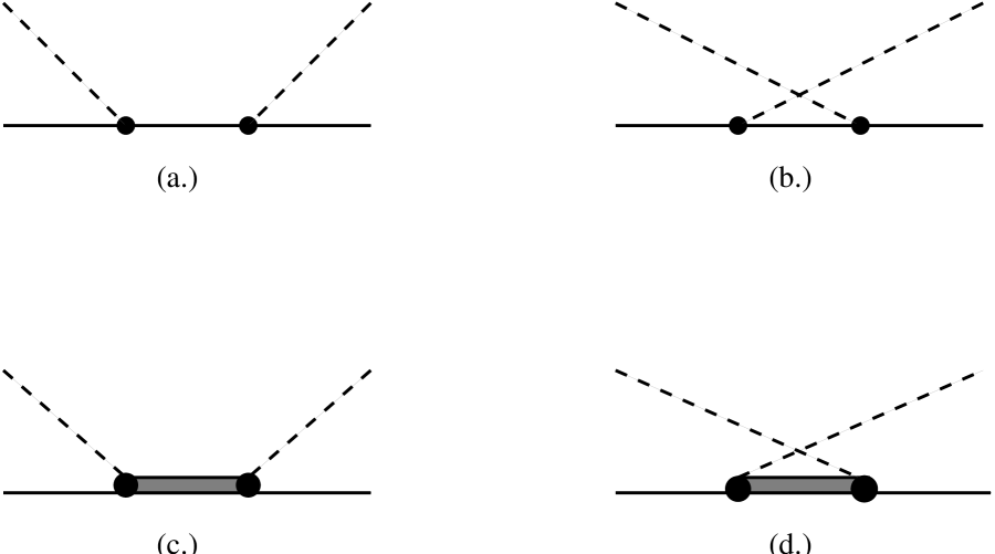
FIG. 1.: Driving terms for pion-nucleon scattering: a.) the direct nucleon term, b.) the crossed nucleon term, c.) the direct $\Delta$ term and d.) the crossed $\Delta$ term. The combined model for scattering in the $P_{33}$ channel developed here includes b.) and c.) as driving terms for the linear equations.

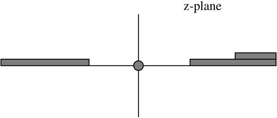
FIG. 2.: Analytic structure of the pion-nucleon scattering amplitude in the complex $W_{q}\rightarrow z$ plane. The cut along the right-hand axis is composed of an elastic scattering contribution which starts at an energy of $m_{{}_{N}}+m_{\pi}$ together with an inelastic contribution starting at the inelastic threshold. There is a pole at $z=m_{{}_{N}}$ as given in Eq. 9, and a cut along the left-hand axis, the crossed cut. In the model developed here, the left-hand cut is approximated by an increase in the residue of the pole term.

FIG. 3.: The phase shift $\delta_{33}$ in the $P_{33}$ channel versus the center-of-momentum momentum $q$. The dots are the result of the phase shift analysis of Ref. [7]. The solid curve is the results of the Chew-Low model and the dashed curve is the results for the Lee model.

FIG. 4.: The same as Fig. 3 except the quantity $q^{3}\,\cot\delta/(W_{q}-m_{{}_{N}})$ is presented.

FIG. 5.: The same as Fig. 3 except the curves are the results of the combined model. The solid curve corresponds to $\beta=$ 1100 MeV/c, the long-dashed curve to $\beta=$ 800 MeV/c, the short-dashed curve to $\beta=$ 500 MeV/c, and the dot-dashed curve to $\beta=$ 400 MeV/c.

FIG. 6.: The same as Fig. 5 except the quantity $q^{3}\,\cot\delta/(W_{q}-m_{{}_{N}})$ is presented.

FIG. 7.: The same as Fig. 5 except the total elastic cross section, $\sigma_{e\ell}^{tot}$, in the $P_{33}$ channel is presented.

FIG. 8.: The coupling constants as a function of the form-factor cutoff parameter $\beta$ for values which fit the $P_{33}$ data. The solid curve is the unrenormalized nucleon coupling $\lambda_{{}_{N}}^{(0)}$, the dashed curve is the unrenormalized $\Delta$ coupling constant $\lambda_{\Delta}^{(0)}$, and the dot-dashed curve is the renormalized nucleon coupling constant $\lambda_{{}_{N}}$.

FIG. 9.: The bare masses, i.e. the masses in the absence of meson couplings, of the nucleon, solid curve, and the $\Delta$, dashed curve, as a function of the form-factor cutoff parameter $\beta$.

TABLE I.: Typical sets of parameters (the form-factor cutoff $\beta$, the unrenormalized coupling constants $\lambda^{(0)}_{i}$, and unrenormalized $\Delta$ mass $m_{\Delta}^{(0)}$) which produce fits to the $P_{33}$ phase shifts. Also given for each fit are two calculated parameters, $\lambda_{{}_{N}}$ the renormalized pion-nucleon coupling strength, and $m_{{}_{N}}^{(0)}$ the bare nucleon mass. These sets of parameters correspond to the curves depicted in Figs. 5–7. The numbers are given to an accuracy such that the results of this work can be reproduced.

$\beta$ (MeV/c)	$\lambda_{{}_{N}}^{(0)}$ (MeV-1)	$\lambda_{\Delta}^{(0)}$ (MeV-1)	$\lambda_{{}_{N}}$ (MeV-1)	$m_{{}_{N}}^{(0)}$ (MeV)	$m_{\Delta}^{(0)}$ (MeV)
400	$8.28\times 10^{-3}$	$1.02\times 10^{-2}$	$1.03\times 10^{-3}$	962	1294
500	$7.77\times 10^{-3}$	$6.62\times 10^{-3}$	$1.17\times 10^{-3}$	1005	1372
800	$5.34\times 10^{-3}$	$1.98\times 10^{-3}$	$1.19\times 10^{-3}$	1198	1662
1100	$4.57\times 10^{-3}$	$3.33\times 10^{-4}$	$1.12\times 10^{-3}$	1397	1623