Casimir Interaction among Objects Immersed in a Fermionic Environment

Abstract

Using ensembles of two, three and four spheres immersed in a fermionic background we evaluate the (integrated) density of states and the Casimir energy. We thus infer that for sufficiently smooth objects, whose various geometric characteristic lengths are larger then the Fermi wave length one can use the simplest semiclassical approximation (the contribution due shortest periodic orbits only) to evaluate the Casimir energy. We also show that the Casimir energy for several objects can be represented fairly accurately as a sum of pairwise Casimir interactions between pairs of objects.

In 1948 Casimir predicted the existence of a very peculiar effect, the attraction between two metallic parallel plates in vacuum [1]. The existence of such an attraction has been confirmed experimentally with high accuracy only recently [2]. The origin of this attractive force can be traced back to the modification of the spectrum of zero point fluctuations of the electromagnetic field. Similar phenomena are expected to exists for various other (typically bosonic) fields [3, 4] and the corresponding forces are referred to as Casimir or fluctuating interactions. A related interaction arises when the space is filled with (noninteracting) fermions, which is particularly relevant to the physics of neutron stars [5, 6] and quark gluon plasma [7]. Spin–orbit interaction will be neglected as well. One of the simplest cases corresponds to nuclei embedded in a neutron gas. These however could be replaced with buckyballs immersed in an electron gas, in liquid mercury for example. Particularly attractive candidates for the study of this type of Casimir effects in essentially perfect degenerate fermi systems are the dilute atomic Fermi condensates [8].

In the case of two parallel impenetrable planes, dimensional arguments suggest that the dependence of the Casimir energy for fermions on the distance between the two planes has the form

$$E_{C}=\mu F(k_{F}d),$$ (1)

where $\mu=\hbar^{2}k_{F}^{2}/2m$ is the chemical potential, $k_{F}$ is the Fermi wave vector and $d$ is the distance between the two planes. For this simple geometry it is straightforward to evaluate the function $F(k_{F}d)$ [5]. One has to be careful and specify whether the calculation should be performed at fixed particle number or fixed chemical potential, as one can easily show that the Casimir energy has a different behavior in these two limits.

For more complicated geometries the evaluation of the Casimir energy is generally a rather involved, even though straightforward, numerical procedure. Our main goal is to reach a qualitative understanding of the Casimir energy in the case of complicated geometries. We shall consider mainly two obvious limits, when the objects immersed in the Fermi environment are either much smaller or much larger than the Fermi wave length. The limit of small scatterers is relatively easy to treat and is considered mostly for the completeness of the analysis. We show here that the case of large scatterers can be treated quite accurately using semiclassical methods at practically all separations. The most important conclusion we are able to draw from our study however is that the Casimir interaction energy in the case of more than two scatterers can be evaluated quite accurately as a sum of pairwise interactions between these scatterers. This conclusion comes to some extent as a surprise, since it is known that Casimir energy is not pairwise additive, in other words, the interaction among extended objects cannot be evaluated as a sum of pairwise interactions, see e.g. Ref. [3, 4].

Let us consider at first the case of two impenetrable spheres of radius $a$ at a distance $r\geq 2a$ between their centers. In order to calculate the Casimir energy we shall represent the sufficiently smoothed fermion density of states (smoothing is over an energy interval larger than the level spacing in the volume $V$ of the entire system):

$$g(\varepsilon,a,r)=g_{0}(\varepsilon)+g_{W}(\varepsilon,a)+g_{C}(\varepsilon,a,r),$$ (2)

where $g(\varepsilon,a,r)$ is the total fermion density of states, $g_{0}(\varepsilon)$ is the density of states in the absence of scatterers (ideal Fermi gas), $g_{W}(\varepsilon,a)$ is the correction to the density of states arising from the presence of two spheres infinitely apart from each other and $g_{C}(\varepsilon,a,r)$ is the remaining part, which is of central interest to us here (in the following we shall not make explicit the $a$– or $r$–dependence, but show only the energy ($\varepsilon$–) dependence).

In the case of $N$ scatterers the Krein formula [9, 10] provides a link between the $N$–body scattering matrix $S_{N}(\varepsilon)$ and the change in the density of states due to the presence of $N$ scatterers, namely

$$\delta g(\varepsilon)=g(\varepsilon)-g_{0}(\varepsilon)=\frac{1}{2\pi i}\;\frac{d\ln\det S_{N}(\varepsilon)}{d\varepsilon}.$$ (3)

Following Refs. [11], the determinant of the $S_{N}(\varepsilon)$–matrix can be represented as follows

$$\delta g(\varepsilon)=\frac{1}{2\pi i}\;\frac{d\ln\det S_{N}(\varepsilon)}{d\varepsilon}=g_{W}(\varepsilon)+g_{C}(\varepsilon)$$ (4)

$$=\frac{1}{2\pi i}\frac{d}{d\varepsilon}\ln\left[\prod_{j=1}^{N}\det S_{1}(j,\varepsilon)\right]+\frac{1}{2\pi i}\frac{d}{d\varepsilon}\ln\left[\frac{\det M^{\dagger}(\varepsilon^{*})}{\det M(\varepsilon)}\right],$$ (5)

where $M(\varepsilon)$ is a Koringa–Kohn–Rostoker (KKR) multiple scattering matrix [12]. $g_{W}(\varepsilon)$ determines the change in the density of states due to the presence of isolated scatterers, which in case of large scatterers is given basically by a Weyl formula, see Refs. [13, 14] for various examples and general formulas. $g_{C}(\varepsilon)$, which is determined by the multiple scattering KKR–matrix $M(\varepsilon)$, vanishes in the limit of infinitely separated scatterers and is the only part of the density of states which depends on the relative arrangement of the scatterers. The Casimir energy at fixed particle number can then be introduced as

$$E_{C}=\int_{-\infty}^{\mu}\varepsilon g(\varepsilon)d\varepsilon-\int_{-\infty}^{\mu_{0}}\varepsilon[g_{0}(\varepsilon)+g_{W}(\varepsilon)]d\varepsilon$$ (6)

$$\approx\int_{-\infty}^{\mu_{0}}(\varepsilon-\mu_{0})g_{C}(\varepsilon)d\varepsilon=-\int_{-\infty}^{\mu_{0}}{\cal{N}}_{C}(\varepsilon)d\varepsilon,$$ (7)

$${\cal{N}}=\int_{-\infty}^{\mu}g(\varepsilon)d\varepsilon=\int_{-\infty}^{\mu_{0}}[g_{0}(\varepsilon)+g_{W}(\varepsilon)]d\varepsilon,$$ (8)

$${\cal{N}}_{C}(\varepsilon)=\int_{-\infty}^{\varepsilon}d\epsilon g_{C}(\epsilon),$$ (9)

where the omitted terms are ${\cal{O}}(V^{-1})$. ${\cal{N}}$ is the total number of fermions, $\mu$ and $\mu_{0}$ are the values for the chemical potential with the scatterers at finite and infinite separation from each other respectively and ${\cal{N}}_{C}(\varepsilon)$ is the relevant correction to the integrated density of states. Strictly speaking, the quantities $g(\varepsilon)$ and $g_{0}(\varepsilon)$ are infinite, as they are proportional to the volume $V$ of the entire space. This redundant divergence can be handled easily by considering first a very big box, the volume of which is subsequently taken to infinity. One can then show that $E_{C}$ has a well defined and finite value in this limit.

Using the explicit formulas for the KKR–matrix from Ref. [11], one can compute numerically $g_{C}(\varepsilon)$ for various arrangements of hard spherical (or circular in 2D) scatterers. It is possible to obtain significantly simpler expressions for the (integrated) density of states in the limit of very small and very large scatterers. If the wave length $\lambda=2\pi/k$ ($\varepsilon=\hbar^{2}k^{2}/2m$) is much larger than the radii of the scatterers and the scatterers do not overlap then one can show that the KKR–matrix $M(\varepsilon)$ is given by (see [15] for the analog in the 2D case)

$$[M(\varepsilon)]_{nm}\approx\delta_{nm}-(1-\delta_{nm})f_{n}(\varepsilon)\frac{\exp(ikr_{nm})}{r_{nm}},$$ (10)

where the indices $n,m=1,\dots,N$ run over the scatterers, $r_{nm}$ is the distance between the centers of the $n$–th and $m$–th scatterers, $f_{n}(\varepsilon)$ is the $s$–wave scattering amplitude on the $n$–th scatterer. In the case of two spheres of radius $a$, with their centers $r$ apart ($r\gg a$) one obtains

$${\cal{N}}_{C}(\varepsilon)=\nu\frac{a^{2}}{\pi r^{2}}\sin[2k(r-a)]+{\cal{O}}\left((ka)^{3},\frac{a^{4}}{r^{4}}\right),$$ (11)

where $\nu$ is the spin degeneracy factor. The next order correction arises from $p$–wave scattering. In the case of a finite radius $a$, one can use the Gutzwiller trace formula to determine this correction to the (integrated) density of states semiclassically ($scl$) [14]

$$\delta g_{scl}(\varepsilon)=\nu\sum_{po}\frac{(-1)^{m_{po}}T_{ppo}}{\pi\hbar\sqrt{|\det(M_{po}\mbox{$-$}1)|}}\cos\left(\frac{S_{po}}{\hbar}\right),$$ (12)

$${\cal{N}}_{scl}(\varepsilon)=\nu\sum_{po}\frac{(-1)^{m_{po}}}{n\pi\sqrt{|\det(M_{po}\mbox{$-$}1)|}}\sin\left(\frac{S_{po}}{\hbar}\right),$$ (13)

where the summation is over periodic orbits ($po$), $T_{ppo}$ and $n$ are the period and number of repetitions of the primitive periodic orbit ($ppo$), $M_{po}$, $S_{po}$ and $m_{po}$ are the stability matrix, classical action and Maslov index (which counts the number of bounces under Dirichlet boundary conditions) of the $po$ [14]. Taking into account only the contribution arising from the single $po$ of length $2(r-2a)$, with no repetitions, one derives the following result

$${\cal{N}}_{C}(\varepsilon)\approx\nu\frac{a^{2}}{4\pi r(r-2a)}\sin[2k(r-2a)].$$ (14)

At large distances ($r\gg a$) the leading term in both cases (small and large scatterers) has the same analytical structure, apart from an overall numerical factor. The $kr\gg 1$ limit of Rel. (14) can be reproduced from the KKR–matrix in the case of large spheres ($ka>1$) as well. One can expect that the semiclassical result (14) is reasonably accurate when the reduced action along the classical $po$ is larger than unity, i.e. when $S_{po}/\hbar=2k(r-2a)>1$, and that this approximation should fail when the two spheres are very close. Surprisingly however, at smallest separations when $r-2a\ll a$ the semiclassical estimate is only about 30% lower than the exact result. For $2k(r-2a)>1$ the semiclassical expression (14) is very close to the exact numerical result obtained using the KKR–matrix, if the spheres are large ($ka>1$), see Fig. 1. When $ka\gg 1$ a large number of partial waves contribute, which renders thus the semiclassical limit valid. One can show, using arguments along the lines in Ref. [16], that the contribution arising from creeping orbits are exponentially suppressed, which is intuitively expected. The contributions arising from repetitions of the primitive periodic orbit are relatively small, because the long orbits and the repetitions of a primitive orbit are less stable in 3D than in 2D. For this reason the simplest semiclassical approximation for the density of states, and consequently for the Casimir energy, are more accurate for spheres than for cylinders.

Our findings suggest that for more complicated geometries, if the curvature radii are larger than the wave length, one can safely evaluate the density of states using the contributions arising from short primitive periodic orbits only, without any repetitions. If the curvature radii are smaller than the wave length then the alternative simple approximation of small scatterers could be used. Using Eq. (14) one can now easily derive an approximate, but rather accurate, expression for the Casimir energy for two large spheres ($k_{F}a>1$)

$$E_{C}\approx-\nu\mu\frac{a^{2}}{2\pi r(r-2a)}j_{1}[2k_{F}(r-2a)],$$ (15)

where $j_{1}(x)$ is the spherical Bessel function.

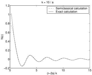
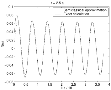
FIG. 1.: The correction to the number of states $N_{C}(\varepsilon)$ as a function of $r-2a$ in the upper part and as a function of $k$ in the lower part for $\nu=1$

Under the same approximations the Casimir energy of a large sphere at a distance $r$ from an infinite plane reads

$$E_{C}\approx-\nu\mu\frac{a}{2\pi(r-a)}j_{1}[2k_{F}(r-a)].$$ (16)

One can naturally expect that if a standing wave with the Fermi momentum could be formed in between the two spheres then the total energy of the system is at a (local) minimum, which thus explains the oscillatory character of this interaction.

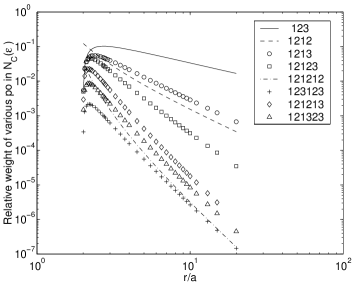
FIG. 2.: The relative amplitude of the contribution to the semiclassical density of states (13) of $n$–bounce periodic orbits for the system of three identical spheres, situated at the vertices of an equilateral triangle, as a function of the distance between two spheres $r/a(r\geq 2a)$ as compared to the amplitude of the 2–bounce orbit, including the corresponding degeneracies. In the legend 123 denotes an orbit starting at the sphere 1, followed by a bounce off the sphere 2, then off the sphere 3 and ending on sphere 1, and so forth.

Let us consider now the case of three and four spheres. The semiclassical picture makes particularly transparent the reason why, strictly speaking, the Casimir energy cannot be represented as a sum of pairwise interactions. Each primitive periodic orbit and its repetitions give rise to an additive contribution to the density of states, see Eq.(13), and thus to the Casimir energy (6). For three or more objects there are periodic trajectories (or standing waves) bouncing off three or more such objects and thus the contribution to the density of states and to the Casimir energy due to such orbits depends on the relative arrangement of three or more objects, thus leading to genuine three and more body interactions. We determined however that the contribution of three or more bounce orbits to the density of states, and thus to the Casimir energy as well, is never dominant. (NB Our analysis and conclusions refer to the global domain of the system always and not to the fundamental domain or to the one–dimensional representations of a symmetry reduced problem.) An analysis of the stability matrix of an $n$–bounce orbit shows that its contribution to the integrated density of states at large distances is proportional to $1/L^{n}$, where $L$ is the length of the orbit, if all the legs of the orbit are comparable in length, see Fig. (2). Any person who ever played pool (thus in 2D) knows instinctively that long shots are more difficult than short ones and that the most difficult shots are the many–bounce shots. In 3D and higher dimensions orbits are typically more unstable than in 2D. An exact evaluation of the stability matrix for various periodic trajectories shows that even at small separations the contributions of 2–bounce periodic orbits dominate over those of three or more bounce periodic orbits. The 3–bounce orbit gives the largest contribution, an approximately 10 % corrections, at $r\approx 2.5a$. As one can also judge from Figs. (3) the role of the orbits bouncing among three or more objects is never too large. The Casimir energy for three identical spheres (at the vertices of an equilateral triangle) satisfies the approximate relation $E_{3}\approx 3E_{2}$ and correspondingly in the case of four identical spheres (at the vertices of a tetrahedron) one has $E_{4}\approx 6E_{2}\approx 2E_{3}$, where $E_{N}$ stands for the Casimir energy of $N$ spheres, with high accuracy if $k_{F}a\gg 1$. For $k_{F}a\leq 1$ corrections could reach 10% for three and 25 % for four spheres.

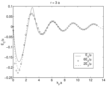
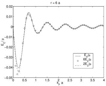
FIG. 3.: The ratio of the exact Casimir energy and chemical potential $E_{C}/\mu$ for four spheres and computed as a sum of the exact contributions due to pairs or triplets of spheres for two different separations.

We presented here results only for the symmetric arrangement of the spheres due to the lack of space. Various asymmetrical configurations of three and four spheres show the same general pattern, namely that the correction to the integrated density of states ${\cal{N}}_{C}(\varepsilon)$ can be represented fairly accurately as a sum of the corresponding corrections for pairs of spheres. Obviously, one can replace the spheres with other objects, with curvature radii larger than the Fermi wave length. The pairwise additivity of the Casimir interaction is reasonably well satisfied as well for the case of point scatterers, as one can easily check using Eq. (10). We thus conclude that genuine many–body Casimir interactions are relatively short ranged and that two–body interactions strongly dominate – even for small separations.

We thank Piotr Magierski for discussions. This work has been supported financially partially by DoE.

REFERENCES

- [1] H.B.G. Casimir, Proc. K. Ned. Akad. Wet. 51, 793 (1948).
- [2] S.K. Lamoreaux, Phys. Rev. Lett, 78, 5 (1997); 81, 5475(E) (1998); U. Mohideen and A. Roy, Phys. Rev. Lett. 81, 4549 (1998).
- [3] V.M. Mostepanenko and N.N. Trunov, The Casimir Effect and its Applications. Clarendon Press, Oxford (1997); M.E. Fisher and P.G. de Gennes, C.R. Acad. Sci. Ser. B 287, 207 (1978); A. Hanke et al., Phys. Rev. Lett. 81, 1885 (1998) and references therein.
- [4] M. Kardar and R. Golestanian, Rev. Mod. Phys. 71, 1233 (1999) and references therein.
- [5] A. Bulgac and P. Magierski, Nucl. Phys. A383, 695 (2001) and astro–ph/0002377 and references therein.
- [6] A. Bulgac et al., in Proc. Intern. Work. on Collective excitations in Fermi and Bose systems, eds. C.A. Bertulani and M.S. Hussein (World Scientific, Singapore 1999), pp 44–61 and nucl–th/9811028; Y. Yu et al., Phys. Rev. Lett. 84, 412 (2000) and nucl–th/9902011.
- [7] G. Neergaard and J. Madsen, Phys. Rev. D 62, 034005 (2000) and earlier references therein.
- [8] B. DeMarco and D. S. Jin, Science 285, 1703 (1999).
- [9] M.G. Krein, Mat. Sborn. (N.S.) 33, 597 (1953); Sov. Math.-Dokl. 3, 707 (1962); M.Sh. Birman and M.G. Krein, Sov. Math.-Dokl. 3, 740 (1962); W. Thirring, “Quantum Mechanics of Atoms and Molecules”, Springer–Verlag, New York (1981), ch. 3.6; M.Sh. Birman and D.R. Yafaev, St. Petersburg Math. J. 4, 833 (1993).
- [10] E. Beth and G.E. Uhlenbeck, Physica 4, 915 (1937); K. Huang, Statistical Mechanics, John Wiley & Sons, New York (1987), ch. 10.3; J. Friedel, Nuovo Cim. Ser. 10 Suppl. 7, 287 (1958). These results for the correction to the density of states are particular cases of the Krein formula [9].
- [11] M. Henseler, A. Wirzba and T. Guhr, Ann. Phys. 258, 286 (1997); A. Wirzba, Phys. Rep. 309, 1 (1999).
- [12] J. Koringa, Physica 13, 392 (1947); W. Kohn and N. Rostoker, Phys. Rev, C94, 1111 (1954); A. Gonis and W.H. Butler, Multiple Scattering in Solids, Springer, New York (2000).
- [13] H.P. Baltes and E.R. Hilf, Spectra of Finite Systems, Wissenschaftsverlag, Mannheim, Wien, Zürich, Bibliographisches Institut, (1976).
- [14] M. Brack and R.K. Bhaduri, Semiclassical Physics, Addison Wesley Publishing Company, Inc. (1997).
- [15] P. E. Rosenqvist et al., J. Phys. A 29, 5441 (1996).
- [16] G. Vattay et al., Phys. Rev. Lett. 73, 2304 (1994).