Event-by-event analysis of ultra-relativistic heavy-ion collisions in smoothed particle hydrodynamics

Abstract

The method of smoothed particle hydrodynamics (SPH) is applied for ultra-relativistic heavy-ion collisions. The SPH method has several advantages in studying event-by-event fluctuations, which attract much attention in looking for quark gluon plasma (QGP) formation, because it gives a rather simple scheme for solving hydrodynamical equations. Using initial conditions for Au+Au collisions at RHIC energy produced by NeXus event generator, we solve the hydrodynamical equation in event-by-event basis and study the fluctuations of hadronic observables such as $dN/dy$ due to the initial conditions. In particular, fluctuations of elliptic flow coefficient $v_{2}$ is investigated for both the cases, with and without QGP formation. This can be used as an additional test of QGP formation.

1 Introduction

One of the central issues of the high-energy heavy-ion physics is to investigate the phases of the hadronic and quark matter. Hydrodynamical descriptions[1], which have a rather long history, may be a powerful tool for studying such phase diagrams because we can handle the equation of state directly in the model. However, to extract precisely information about the equation of state, we must be careful in comparing the model predictions with experimental data because procedures of event averaging may make signal of QGP ambiguous.

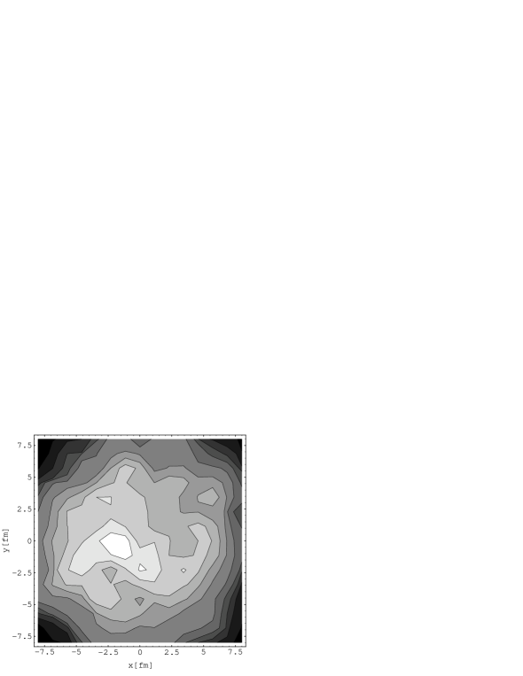
Figure 1: Initial energy density (counter plot $z=0~{}fm$ plane) of a typical event of Au+Au collision at energy $\sqrt{s}=200A~{}GeV$, impact parameter $b=0fm$, produced by NeXus event generator[3].

Event-by-event analysis[2] is one of promising ways to extract clear information from the experimental data, in particular at RHIC and LHC energy regions. The fluctuations at the initial stage (for example, the initial energy density fluctuation) must affect the formation of QGP and the later space-time evolution of the whole system. Fig.1 shows the energy density (counter plot, at $z=0~{}fm$ plane) for a Au+Au collision at $\sqrt{s}=200A~{}GeV$, $b=0~{}fm$, produced by NeXus code[3]. As shown in Fig.1, the fluctuations at the initial stage of relativistic heavy-ion collisions are not negligible. To achieve an event-by-event analysis using relativistic hydrodynamical model, the numerical code must deal with arbitrary initial conditions and equation of state with suitable calculational speed and precision. The method of smoothed particle hydrodynamics (SPH)[4], which was first introduced for astrophysical applications[5], satisfy such requirements. The main characteristic of SPH is the introduction of “particles” attached to some conserved quantity which are described in terms of discrete Lagrangian coordinates. This feature of the model enables to easily carry out calculations of the ultra-relativistic heavy-ion collisions, which is accompanied by prominent longitudinal expansion. Another advantage of using SPH method is that we can choose a suitable precision in solving hydrodynamical equations because of the smoothing kernel, which allows to smooth out often unnecessary very precise local aspects and then achieve a reduction of computational time. This is a very profitable point in the event-by-event analysis.

In the following section, we briefly formulate the entropy-based SPH, using the variational approach[6]. In Sec.3, to check the performance of SPH, we apply it for solving problems of relativistic hydrodynamics whose solutions are known analytically or numerically. Then, in Sec.4, we demonstrate hydrodynamical evolutions of both resonance gas and quark gluon plasma starting from the same simple initial conditions. In Sec.5, after giving a brief explanation how to take the initial conditions of NeXus into our code, we present typical hydrodynamical evolution of an event at RHIC energy. To introduce freeze-out process into our code, we formulate Cooper-Frye formula in terms of SPH and show several results on single-particle spectrum in Sec.6. Then, we study the event-by-event fluctuation of elliptic flow coefficient $v_{2}$[7] at RHIC energy[8] in Sec.7, showing that the dispersion is large and it does depend on the equation of state used. Finally we close our discussions with some concluding remarks.

2 Relativistic SPH equations

2.1 SPH representation

To specify the hydrodynamical state of a fluid, we need to locally know the thermodynamical quantities such as the energy density $\varepsilon$ and the collective velocity field, besides equation of state of the fluid. If local thermal equilibrium is well established, the thermodynamical variables may be expressed by smooth functions of the coordinates. Let us choose $N$ space points to specify the state of the whole system. To know the physical quantities in other space points, we may use an interpolation using the known $N$ points. (Hereafter we use the word ‘particles’ instead of ‘points’.)

In SPH, for an arbitrary extensive thermodynamical quantity of $A$, the density (in the space-fixed frame) $a^{*}$ is parametrized in the following way:

$$a^{*}(\mbox{\boldmath{$x$}},t)=\sum_{i}^{N}\nu_{i}~{}W(\mbox{\boldmath{$x$}}-\mbox{\boldmath{$x$}}_{i}(t);h)~{},$$ (1)

where $W(\mbox{\boldmath{$x$}}-\mbox{\boldmath{$x$}}_{i}(t);h)$ is a positive definite kernel function with the properties

$$\int\!d\mbox{\boldmath{$x$}}^{\prime}~{}W(\mbox{\boldmath{$x$}}^{\prime}-\mbox{\boldmath{$x$}})\equiv 1\quad\quad\mbox{and}\quad\quad W(\mbox{\boldmath{$x$}}^{\prime}-\mbox{\boldmath{$x$}},h)=\delta(\mbox{\boldmath{$x$}}^{\prime}-\mbox{\boldmath{$x$}})\quad\mbox{when $h\to 0$}~{},$$

where $h$ is a smoothing-scale parameter. Using the normalization above, we have

$$A_{total}=\int\!d^{3}\mbox{\boldmath{$x$}}~{}a^{*}(\mbox{\boldmath{$x$}},t)=\sum_{i}^{N}\nu_{i}~{}.$$ (2)

From eq.(2) the quantity $\nu_{i}$ can be interpreted as a portion of $A$ which is carried by the $i$th particle. Its velocity, identified as the velocity of the fluid at $\mbox{\boldmath{$x$}}_{i}(t)$, satisfies

$$\mbox{\boldmath{$v$}}_{i}(t)=\frac{d\mbox{\boldmath{$x$}}_{i}(t)}{dt}~{}.$$ (3)

If $A$ is a conserved quantity, $\nu_{i}$ must be constant in time. In this case, from eqs.(1) and (3), we obtain

$$\frac{\partial}{\partial t}~{}a^{*}(\mbox{\boldmath{$x$}},t)=-\mbox{\boldmath{$\nabla$}}\cdot\mbox{\boldmath{$j$}}(\mbox{\boldmath{$x$}},t)~{},$$ (4)

where

$$\mbox{\boldmath{$j$}}(\mbox{\boldmath{$x$}},t)=\sum_{i}~{}\nu_{i}\mbox{\boldmath{$v$}}_{i}(t)~{}W(\mbox{\boldmath{$x$}}-\mbox{\boldmath{$x$}}_{i}(t);h)$$ (5)

is interpreted as the current density of the thermodynamical quantity $A$ and eq.(4) is then the corresponding continuity equation.

2.2 Equations of motion for SPH particles

To know the time evolution of the fluid, we have to find the equation of motion for each SPH particle. It can be obtained by the variational method[6] with the following Lagrangian[4]

$$L_{\mbox{\tiny SPH}}(\{\mbox{\boldmath{$x$}}_{i},\mbox{\boldmath{$v$}}_{i}\})=-\sum_{i}\nu_{i}~{}\frac{\varepsilon_{i}}{a^{*}_{i}}$$ (6)

It should be noted here that the factor $\nu_{i}/a^{*}_{i}$ can be regarded as the volume $V_{i}$ (in the space-fixed frame) occupied by the $i$th ‘particle’. Then each term in eq.(6) is equal to $E_{i}/\gamma_{i}$, where $E_{i}$ and $\gamma_{i}$ are the energy (in the rest frame) and the gamma factor of the $i$th particle, respectively. Then we also write

$$L_{\mbox{\tiny SPH}}(\{\mbox{\boldmath{$x$}}_{i},\mbox{\boldmath{$v$}}_{i}\})=-\sum_{i}\frac{E_{i}(\mbox{\boldmath{$x$}}_{i},\mbox{\boldmath{$v$}}_{i})}{\gamma_{i}(\mbox{\boldmath{$v$}}_{i})}~{}.$$ (7)

The equations of motion of SPH particles are obtained minimizing the action $I_{\mbox{\tiny SPH}}$ with respect to $\{\mbox{\boldmath{$x$}}_{i}\}$ with the constraint given by eq.(3) taken into account

$$\delta I_{\mbox{\tiny SPH}}(\{\mbox{\boldmath{$x$}}_{i},\mbox{\boldmath{$v$}}_{i}\})=-\delta\int\!\!dt~{}~{}\frac{E_{i}}{\gamma_{i}}=0~{}.$$ (8)

Using the adiabatic condition

$$\delta E_{i}=P\delta V_{i}\quad=P_{i}~{}\delta\Big{(}\frac{\nu_{i}\gamma_{i}}{a^{*}_{i}}\Big{)}~{},$$ (9)

we obtain

$$\frac{d}{dt}(\nu_{i}\frac{P_{i}+\varepsilon_{i}}{a_{i}}\gamma_{i}\mbox{\boldmath{$v$}}_{i})+\sum_{j}\nu_{j}\bigg{[}\frac{P_{i}}{{a^{*}_{i}}^{2}}+\frac{P_{j}}{{a^{*}_{j}}^{2}}\bigg{]}~{}\mbox{\boldmath{$\nabla$}}W(\mbox{\boldmath{$x$}}_{i}-\mbox{\boldmath{$x$}}_{j};h)=0~{},$$ (10)

where $P_{i}$ is the pressure. Because of the adiabatic condition, eqs.(10) are the equations of motion for the ideal fluid. For the extension to the non-adiabatic case, see ref.[4].

2.3 Entropy based SPH in general coordinate system

As a possible candidate for the thermodynamical extensive quantity $a^{*}$, we may consider baryon number density, entropy density, energy density and so on. In the case of energy density, we have (cf. eq.(6) and (7))

$$\nu_{i}=E_{i}(\mbox{\boldmath{$x$}}_{i},\mbox{\boldmath{$v$}}_{i})~{}.$$ (11)

However, this is only the internal energy, so $\nu_{i}$ is not constant with respect to the variation of ${\mbox{\boldmath{$x$}}_{i}}$ in eq.(8), introducing an additional complication without any practical merit. On the other hand, for entropy or baryon number density, for example, $\nu_{i}$ can be kept constant. Since we will apply SPH to ultra-relativistic heavy-ion collisions, baryon number density is not so suitable choice because it is expected to be very small in the central rapidity region. Let us choose the entropy density for $a^{*}$ in eq.(1).

In relativistic heavy-ion collisions, initial conditions of fluid are often given at constant $\tau\equiv\sqrt{t^{2}-z^{2}}$. Then, it is convenient to formulate SPH in the coordinates

$$x^{0}\equiv\tau=\sqrt{t^{2}-z^{2}},~{}~{}x^{1}\equiv x,~{}~{}x^{2}\equiv y,~{}~{}x^{3}\equiv\eta=\frac{1}{2}\ln\frac{t+z}{t-z}~{}~{}.$$ (12)

The SPH equations in generalized coordinate system are easily derived in a similar way[4]. In the case of the coordinate above, the SPH equations of motion should be written as

$$s(\tau,\mbox{\boldmath{$x$}})=\frac{1}{\tau u^{0}}\sum_{i}\nu_{i}W(\mbox{\boldmath{$x$}}-\mbox{\boldmath{$x$}}_{i}:h)~{},$$ (13)

$$\frac{d}{d\tau}(\nu_{i}\frac{P_{i}+\varepsilon_{i}}{s_{i}}\gamma_{i}\mbox{\boldmath{$v$}}_{i})+\sum_{j}\frac{\nu_{j}}{\tau}\bigg{[}\frac{P_{i}}{{s_{i}}^{2}{u^{0}_{i}}^{2}}+\frac{P_{j}}{{s_{j}}^{2}{u^{0}_{j}}^{2}}\bigg{]}~{}\mbox{\boldmath{$\nabla$}}W[\mbox{\boldmath{$x$}}_{i}-\mbox{\boldmath{$x$}}_{j};h]=0~{}.$$ (14)

3 Numerical check of SPH

To check the performance of SPH formulated in Sec.2, we applied it to a problem of relativistic hydrodynamics whose solution is known analytically. When the longitudinal rapidity $\alpha$ and the transverse one $\beta$ are given as

$$\alpha\equiv\eta,\quad\beta\equiv\frac{1}{2}\ln\frac{\tau+\sqrt{x^{2}+y^{2}}}{\tau-\sqrt{x^{2}+y^{2}}}~{},$$ (15)

it is known that the entropy density is given by

$$s=\frac{s_{0}}{[\tau^{2}-x^{2}-y^{2}]^{3/2}}~{},$$ (16)

where $s_{0}$ is a constant which is determined by the initial conditions. A comparison of the numerical results by SPH with the analytical solution eq.(16) is shown in Fig.2, where the equation of state used was $c_{s}^{2}=1/3$. It is verified that SPH solves this problem correctly. For a further check, we applied it also to another problem, namely, relativistic hydrodynamics with the longitudinal scaling and the Landau-type initial condition in the transverse directions,

$$\alpha\equiv\eta,\quad\beta\equiv 0~{}.$$ (17)

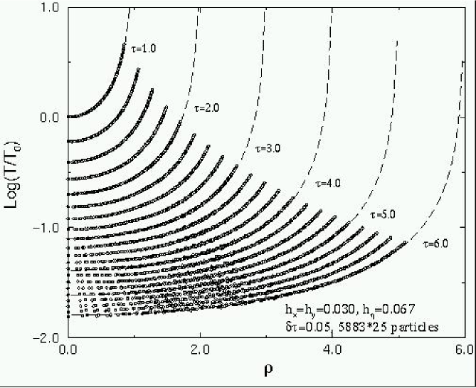
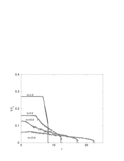
Figure 2: Comparison of results by SPH (open circles) with the analytical solution, eq.(16). The sizes of the parameters $h_{x}(=h_{y})$, $h_{\eta}$ and $d\tau$ used were 0.030, 0.067 and 0.05, respectively.

Figure 3: Numerical results by SPH (open circles) for the problem of longitudinally scaling hydrodynamics using the Landau-type initial conditions in the transverse directions. The solid line has been obtained numerically by Hama and Pottag [9].

Figure 3 shows a comparison of the SPH results with those obtained by Hama and Pottag[9]. The initial conditions and the equation of state used are exactly the same as in ref.[9]. We found that SPH works well also in this problem.

4 Equations of state and hydrodynamical evolutions

To complete the theory of relativistic hydrodynamics, the equation of state (EoS) for the fluid is required. We use two possible EoS in the present study, namely, a resonance gas EoS[10] and an EoS containing both resonance gas and QGP via a first order phase transition[11]. The EoS are parametrized as follows (See also Fig.4.):

$$P/\varepsilon=0.20\mbox{\quad( constant for whole $\varepsilon$~{}region ), }$$ (18)

for the resonance gas (RG) and

$$P/\varepsilon=\left\{\begin{array}[]{ll}0.20&\quad\quad 0.00~{}GeV/fm^{3}~{}<~{}\varepsilon~{}<~{}0.28~{}GeV/fm^{3}\equiv\varepsilon_{1}\\ 0.056/\varepsilon&\quad\quad 0.28~{}GeV/fm^{3}~{}<~{}\varepsilon~{}<~{}1.45~{}GeV/fm^{3}\equiv\varepsilon_{2}\\ 1/3-4B/3\varepsilon&\quad\quad 1.45~{}GeV/fm^{3}~{}<~{}\varepsilon\end{array}\right.$$ (22)

for the quark gluon plasma (QGP) EoS. The bag constant $B=0.32GeV/fm^{3}$ is determined to give the critical temperature $T_{c}=160~{}MeV$. A remark should be made here that when we call QGP EoS, here and in the following sections, we are actually considering all these three states according to the value of $\varepsilon$.

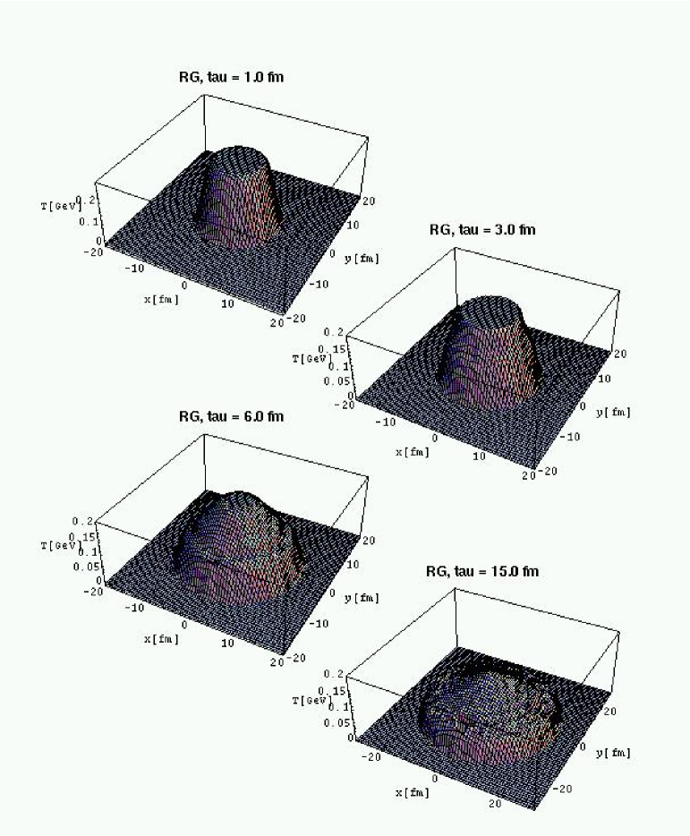
Figure 5: Hydrodynamical evolution (temperature $T~{}[GeV]$ at $z=0fm$ plane) using RG EoS. The smoothing scale parameter $h$ used in $x$-$y$ space is $1.0~{}fm$ and in $\eta$ space $1.0$, respectively.

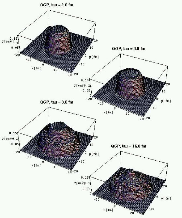
Figure 6: Hydrodynamical evolution (temperature $T~{}[GeV]$ at $z=0fm$ plane) using QGP EoS. At $\tau=2.0~{}fm$, we can observe QGP phase (above $T>T_{c}=0.16~{}GeV$) and mixed phase($T=T_{c}$) clearly. At around $\tau\sim 3~{}fm$, QGP phase almost disappear. Mixed phase survives up to about 25 $fm$.

We show some results of the hydrodynamical evolution using such RG and QGP EoS in Figs. 5 and 6. For the both cases, the initial ($\tau_{0}=1.0~{}fm$) entropy density $s$, longitudinal and transverse rapidity $\alpha$, $\beta$ are set as

$$s=40[1/fm^{3}],\quad\alpha=\eta~{},\quad\beta=0~{}.\quad\mbox{for $\sqrt{x^{2}+y^{2}}<7.0~{}fm$, $|\eta|<7.0$ ~{}.}$$ (23)

As seen in Figs.5 and 6, the space-time evolution of the fluid strongly depends on the EoS. In comparison with the RG case, the temperature of the fluid in QGP EoS drops much slowly due to the existence of the mixed phase, where the pressure is constant.

5 Initial conditions produced by NeXus

The most fundamental assumption of hydrodynamical models is the thermalization of partonic or hadronic systems produced after high-energy heavy-ion collisions. In our study, we set the initial conditions using information from Nexus event generator[3], in the following 2 steps.

1. Align all primary hadrons on the $\tau=\tau_{0}$ hypersurface. Here we assume that the primary hadrons move freely with the momentum $p^{\mu}$. In the present study, we use $\tau_{0}=1.0~{}fm$.

2. The initial energy density and momentum density are estimated using the interpolation kernel $W$.

   $$\varepsilon(\tau_{0};\mbox{\boldmath{$x$}})=\sum_{i}p^{0}_{i}W(\tau_{0},\mbox{\boldmath{$x$}}-\mbox{\boldmath{$x$}}_{i};h)~{},$$

   $$\mbox{\boldmath{$p$}}(\tau_{0};\mbox{\boldmath{$x$}})=\sum_{i}\mbox{\boldmath{$p$}}_{i}W(\tau_{0},\mbox{\boldmath{$x$}}-\mbox{\boldmath{$x$}}_{i};h)~{},$$

   where $\mbox{\boldmath{$x$}}_{i}=(x_{i},y_{i},\eta_{i})$ are the coordinates of the $i$-th primary hadron after the alignment on $\tau=\tau_{0}$. The smoothing scale parameter $h=1~{}fm$ is used, which is the rough size of the hadrons. The collective velocity field is then given by $\mbox{\boldmath{$v$}}(\tau_{0},\mbox{\boldmath{$x$}})=\mbox{\boldmath{$p$}}(\tau_{0},\mbox{\boldmath{$x$}})/\varepsilon(\tau_{0},\mbox{\boldmath{$x$}})$ .

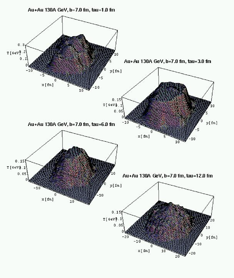
Figure 7: Hydrodynamical evolution (temperature $T~{}[GeV]$) of a typical event in $Au+Au$ collision at energy $\sqrt{s}=130A~{}GeV$ for the impact parameter $b=7.0~{}fm$ (at $z=0~{}fm$, impact parameter direction is parallel to $x$ direction). The initial conditions are produced by NeXus[3]. The EoS used is QGP one.

In Fig.7, we show the hydrodynamical evolution of a typical event of $Au+Au$ collision at energy $\sqrt{s}=130A~{}GeV$ for the impact parameter $b=7.0fm$ given by our hydro code, SPheRIO, connected to the NeXus event generator.

6 Cooper-Frye formula in SPheRIO

The Cooper-Frye formula[12] is widely used in calculations of single particle spectra using hydrodynamical models because of its simplicity. So, as the first trial to evaluating single particle densities, we shall follow it.

In SPH, using eq.(13), the usual Cooper-Frye formula can be rewritten as

$$E\frac{d^{3}N}{d\mbox{\boldmath{$p$}}^{3}}\!\! = \!\!\frac{g}{(2\pi)^{3}}\sum_{j}\nu_{j}\int_{F.O.}\tau dxdyd\eta~{}\frac{\sigma_{\mu}p^{\mu}~{}}{\tau~{}su^{0}}~{}W(\mbox{\boldmath{$x$}}-\mbox{\boldmath{$x$}}_{j}(\tau);h)~{}\frac{1}{e^{u_{\mu}p^{\mu}/T_{\!f}}\mp 1}~{},$$ (24)

where $\sigma_{\mu}$ is defined by

$$\sigma_{\mu}\equiv\Big{(}~{}1,\frac{n_{x}}{n_{\tau}},\frac{n_{y}}{n_{\tau}},\frac{n_{\eta}}{n_{\tau}}~{}\Big{)}$$ (25)

and $n_{\mu}=(n_{\tau},n_{x},n_{y},n_{\eta})$ is the normal vector of the isothermals:

$$n_{\mu}\equiv\Big{(}-\frac{\partial T}{\partial\tau},-\frac{\partial T}{\partial x},-\frac{\partial T}{\partial y},-\frac{\partial T}{\partial\eta}~{}\Big{)}~{}.$$ (26)

The integration is usually done over a constant temperature hypersurface, $T=T_{f}$. When the spline-type kernel function[4, 5] is used, $W(\mbox{\boldmath{$x$}}-\mbox{\boldmath{$x$}}^{\prime};~{}h)=0$ for $|\mbox{\boldmath{$x$}}-\mbox{\boldmath{$x$}}^{\prime}|>2h$. Then, within the approximation of small $h$,

$$E\frac{d^{3}N}{d\mbox{\boldmath{$p$}}^{3}}\!\! \approx \!\!\frac{g}{(2\pi)^{3}}\sum_{j}\nu_{j}\bigg{[}\frac{p^{\mu}}{e^{u_{\mu}p^{\mu}/T_{\!f}}\mp 1}\bigg{]}_{j}\int\tau dxdyd\eta~{}\frac{\sigma_{\mu}~{}}{\tau~{}su^{0}}~{}W(\mbox{\boldmath{$x$}}-\mbox{\boldmath{$x$}}_{j}(\tau_{\mbox{\tiny F}}(\mbox{\boldmath{$x$}}))~{};h)~{}$$ (27)

$$= \!\!\frac{g}{(2\pi)^{3}}\sum_{j}\bigg{[}\frac{p^{\mu}}{e^{u_{\mu}p^{\mu}/T_{\!f}}\mp 1}\bigg{]}_{j}\int~{}dxdyd\eta~{}\frac{\nu_{j}}{~{}su^{0}}~{}\frac{\sigma_{\mu}W(\mbox{\boldmath{$x$}}-\mbox{\boldmath{$x$}}_{j}~{};h)}{|1+v_{j}^{x}\frac{n_{x}}{n_{\tau}}+v_{j}^{y}\frac{n_{y}}{n_{\tau}}+v_{j}^{\eta}\frac{n_{\eta}}{n_{\tau}}|}~{},$$

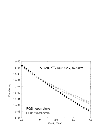
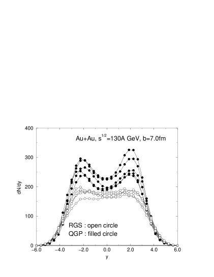
Figure 8: $m_{\mbox{\tiny T}}$-spectra in $Au+Au$ collisions at $\sqrt{s}=130A~{}GeV$, $b=7.0~{}fm$, for 5 events (open circles for RG and filled circles for QGP).

Figure 9: $dN/dy$ in $Au+Au$ collisions at $\sqrt{s}=130A~{}GeV$, $b=7.0~{}fm$, for 5 events (open circles for RG and filled circles for QGP).

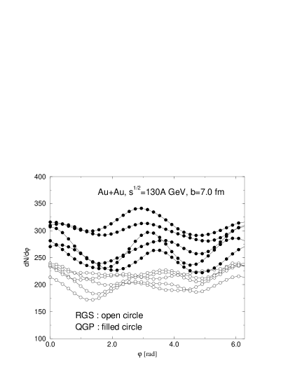
Figure 10: $dN/d\varphi$ in $Au+Au$ collisions at $\sqrt{s}=130A~{}GeV$, $b=7.0~{}fm$, for 5 events (open circles for RG and filled circles for QGP).

where $\mbox{\boldmath{$x$}}_{j}$ gives the point where $j$-th SPH-particle crosses the freeze-out hypersurface. The result of the single-particle spectra, $1/m_{\mbox{\tiny T}}dN/dm_{\mbox{\tiny T}}$, $dN/dy$ and $dN/d\varphi$ for Au+Au collisions at $\sqrt{s}=130A~{}GeV$, $b=7.0~{}fm$ are shown in Figs. 8, 9 and 10, respectively. The freeze-out temperature used is $T_{f}=140~{}MeV$.

7 Event-by-event analysis of hadronic observables

7.1 Elliptic flow coefficient $v_{2}$

The flow phenomena[13] can be important candidates of QGP signals because they may carry much information about EoS during the expansion of quark or hadronic matter. In particular, the elliptic flow coefficients[7] is one of the interesting observables since it is sensitive to the early stage of high-energy heavy-ion collisions. Because it is expected that different EoS responds to the initial fluctuations in different way, the measure of fluctuation, for example, $\delta v_{2}\equiv\sqrt{\langle v_{2}^{2}\rangle-\langle v_{2}\rangle^{2}}$ is also very important. For this purpose, we investigate $v_{2}$ distribution using different EoS. In Figs.11, 12 and Table 1, we show results of the $v_{2}$ distribution for $Au+Au$ collisions at energy $\sqrt{s}=130A~{}GeV$ in RG and QGP EoS cases.

As seen in Table 1, the fluctuations of flow coefficient $v_{2}$ in QGP is about 20 $\sim$ 30% smaller than that in RG (cf. the difference of $\langle v_{2}\rangle$ in RG and QGP. It is about a few %.). The $b$ dependence of $\delta v_{2}$ is also found. Hence, it is expected that $\delta v_{2}$ also brings us useful information to infer on the phase passed in the early stage of high-energy nuclear collisions.

7.2 Fluctuation of the slope parameter

It is also interesting to study the fluctuation of the so-called slope parameter in the transverse momentum spectra. The slope parameter $\tilde{T}$ can be obtained by fitting ${1}/{m_{\mbox{\tiny T}}}{dN}/{dm_{\mbox{\tiny T}}}$ with a function ${\cal N}\exp{[-m_{\mbox{\tiny T}}/\tilde{T}]}$. In the present study, $0<m_{\mbox{\tiny T}}-m_{\pi}<1.0~{}GeV$ interval is used for the fitting. The results are shown in Table 2. We found $\tilde{T}$ and $\delta\tilde{T}$ of QGP is systematically smaller than that of RG.

7.3 Multiplicity fluctuation in the central region

Other interesting measurement may be multiplicity fluctuation. Let us define the fluctuation measure as

$$\delta n(y,\Delta y)\equiv\sqrt{\langle n^{2}(y,\Delta y)\rangle-\langle n(y,\Delta y)\rangle^{2}}$$ (28)

where

$$n(y,\Delta y)=\int_{y-\Delta y}^{y+\Delta y}\!\!\!\!dy~{}\frac{dN}{dy}~{}.$$ (29)

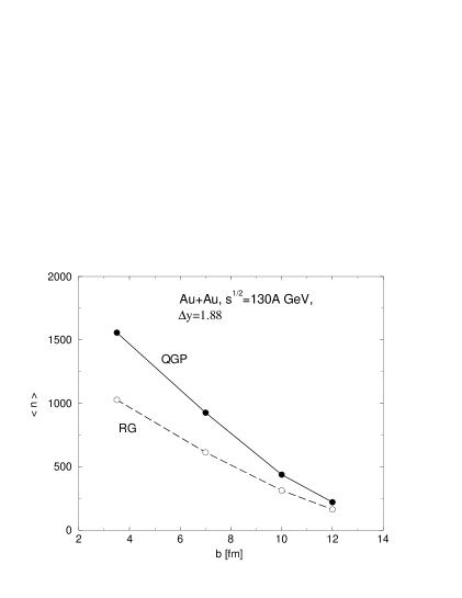
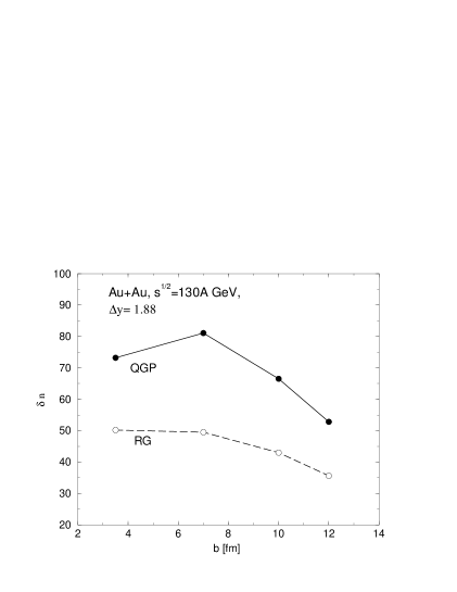
Figure 13: EoS dependence of $\langle n(y,\Delta y)\rangle$ ($y=0,\Delta y=1.875$) as function of impact parameter $b$.

Figure 14: EoS dependence of $\delta n(y,\Delta y)$ ($y=0,\Delta y=1.875$) as function of impact parameter $b$.

We investigate the EoS dependence of the multiplicity fluctuation in two central ($y=0$) rapidity windows $\Delta y$ and as function of the impact parameter $b$. The results are summarized in Table 3. As seen there, the multiplicities and their fluctuations $\delta n$ have a clear EoS dependence. See Figs. 13 and 14. When the initial energy density is bellow $\varepsilon_{2}$ the multiplicity fluctuation with QGP EoS is expected to be larger than that of RG without first order phase transition. This is due to the existence of the mixed phase (see Appendix). The values of ratio $\delta n/\langle n\rangle$ of QGP is slightly larger than those of RG.

8 Concluding remarks and discussions

We developed a new hydrodynamical code, SPheRIO, based on the smoothed particle hydrodynamics (SPH), for studying high-energy heavy-ion collisions in event-by-event basis. In this study, we set the initial conditions based on the results of NeXus event generator and used two types of possible equation of states (EoS), $ie.$, the resonance gas (RG) and quark gluon plasma (QGP) EoS. In the freeze-out process, single particle spectra are calculated by the Cooper-Frye formula for each set of initial conditions and EoS. Analyzing these single particle spectra, the fluctuations in flow coefficients, slope parameter $\tilde{T}$ and multiplicities in the central rapidity regions are investigated at RICH energy.

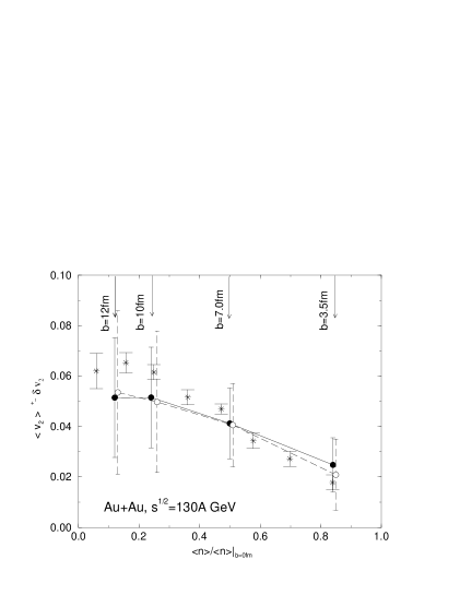
Figure 15: Comparison of our result for $\langle v_{2}\rangle$ with STAR collaboration data[8]. Open circles for RG and filled circles for QGP EoS. Whereas in the data points error bars are shown, in our estimates we have put $\delta v_{2}$.

As seen in the results of Table 1, we found remarkable difference in $\delta v_{2}$ between RG and QGP EoS predictions. This means that the measure of the fluctuations is also helpful to infer the phase passed in the high-energy heavy-ion collisions. In the QGP EoS case, the fluctuations are about $20\sim 30$ % smaller than those in RG case. Our predictions of the average value of $v_{2}$ is shown in Fig.15, compared with STAR Collaboration data[8]. It is seen that the main trend of the data is reproduced, but the fluctuation is quite large.

The fluctuation of the slope parameter $\tilde{T}$ is small, a few % of $\tilde{T}$. We found the fluctuation of multiplicity has a clear EoS dependence. The impact parameter dependence of $\delta n(y,\Delta y)$ can be a good measure for the detection of the first order phase transition.

Acknowledgments: The authors acknowledge stimulating discussions with K. Werner, O. Socolwski Jr and H.J. Drescher. This work was partially supported by FAPESP(contract no.s 98/02249-4 and 98/00317-2), PRONEX(contract no. 41.96.9886.00), FAPERJ(contract no. E-26/150.942/99) and CNPq.

Appendix A Entropy fluctuations in the first order phase transition

A.1 Mixed phase dominant case:

If in the most part of the fluid the energy density at the initial time $\tau_{0}$ varies only in the interval $\varepsilon_{1}<\bar{\varepsilon}(x)<\varepsilon_{2}$, where $\varepsilon_{1}$ and $\varepsilon_{2}$ are the critical densities of the RG and QGP phases, respectively, the produced entropy $S$ of the system is

$$S\!\! = \!\!\int\!d^{3}x~{}s_{1}~{}\Big{[}~{}\frac{\bar{\varepsilon}(x)+\delta\varepsilon(x)}{\varepsilon_{1}}~{}\Big{]}^{1/[1+c_{m}^{2}]}\approx\int\!d^{3}x~{}s_{1}\Big{(}\frac{\bar{\varepsilon}(x)}{\varepsilon_{1}}\Big{)}~{}\Big{[}~{}1+\Big{(}\frac{\delta\varepsilon(x)}{\bar{\varepsilon}(x)}\Big{)}~{}\Big{]}$$

where $c_{m}=0$(constant) is the sound velocity in the mixed phase(Mix) and $s_{1}$ is the critical entropy density corresponding to $\varepsilon_{1}$. $\bar{\varepsilon}(x)$ and $\delta{\varepsilon}(x)$ denote the event averaged energy density and fluctuation, respectively. Here, we assume that $\delta\varepsilon(x)\ll\bar{\varepsilon}(x)$, so that the mixed phase is dominant in all the events. Then, the dispersion of the total entropy $S$ is

$$D^{2}_{Mix}=\langle S^{2}\rangle-\langle S\rangle^{2}\approx\int\!d^{3}x~{}~{}s_{1}^{2}~{}\Big{(}\frac{\bar{\varepsilon}(x)}{\varepsilon_{1}}\Big{)}^{2}~{}\bigg{\langle}\Big{(}\frac{\delta\varepsilon(x)}{\bar{\varepsilon}(x)}\Big{)}^{2}\bigg{\rangle}$$ (A2)

In the case the phase transition is absent, so that the fluid is described by RG EoS, the same events with the same energy distribution and fluctuation gives

$$S_{RG}\!\! = \!\!\int\!d^{3}x~{}s_{1}~{}\Big{[}~{}\frac{\bar{\varepsilon}(x)+\delta\varepsilon(x)}{\varepsilon_{1}}~{}\Big{]}^{1/[1+c_{r}^{2}]}$$ (A3)

$$\approx \!\!\int\!d^{3}x~{}s_{1}\Big{(}\frac{\bar{\varepsilon}(x)}{\varepsilon_{1}}\Big{)}^{5/6}~{}\Big{[}~{}1+\frac{5}{6}\Big{(}\frac{\delta\varepsilon(x)}{\bar{\varepsilon}(x)}\Big{)}-\frac{5}{72}\Big{(}\frac{\delta\varepsilon(x)}{\bar{\varepsilon}(x)}\Big{)}^{2}+\cdots~{}\Big{]}$$

and

$$D_{RG}^{2}=\int\!d^{3}x~{}~{}s_{1}^{2}~{}\Big{(}\frac{\bar{\varepsilon}(x)}{\varepsilon_{1}}\Big{)}^{5/3}~{}\frac{25}{36}\bigg{\langle}\Big{(}\frac{\delta\varepsilon(x)}{\bar{\varepsilon}(x)}\Big{)}^{2}\bigg{\rangle}~{},$$ (A4)

respectively. We used the sound velocity $c_{r}=1/\sqrt{5}$(constant) here. So, the appearance of the mixed phase produces

$$\Delta D^{2}\!\! \equiv D^{2}_{Mix}-D^{2}_{RG}=~{}\!\!\int\!d^{3}x~{}s_{1}^{2}\bigg{\{}~{}\Big{(}\frac{\bar{\varepsilon}(x)}{\varepsilon_{1}}\Big{)}^{2}-\frac{25}{36}\Big{(}\frac{\bar{\varepsilon}(x)}{\varepsilon_{1}}\Big{)}^{5/3}~{}\bigg{\}}\bigg{\langle}\Big{(}\frac{\delta\varepsilon(x)}{\bar{\varepsilon}(x)}\Big{)}^{2}\bigg{\rangle}~{}~{}>0$$

Hence,

$$D_{Mix}^{2}>D^{2}_{RG}~{}.$$ (A5)

A.2 QGP phase dominant case:

If the most part of the fluid is in the QGP phase at initial time $\tau_{0}$, the total produced entropy $S$ of the system is

$$S_{QGP}\!\! = \!\!\int\!d^{3}x~{}s_{2}~{}\Big{[}~{}\frac{\bar{\varepsilon}(x)+\delta\varepsilon(x)}{\varepsilon_{2}}~{}\Big{]}^{1/[1+c_{q}^{2}]}$$ (A6)

$$\approx \!\!\int\!d^{3}x~{}s_{1}\Big{(}\frac{\varepsilon_{2}}{\varepsilon_{1}}\Big{)}~{}\Big{(}\frac{\bar{\varepsilon}(x)}{\varepsilon_{2}}\Big{)}^{3/4}~{}\Big{[}~{}1+\frac{3}{4}\Big{(}\frac{\delta\varepsilon(x)}{\bar{\varepsilon}(x)}\Big{)}-\frac{3}{32}\Big{(}\frac{\delta\varepsilon(x)}{\bar{\varepsilon}(x)}\Big{)}^{2}+\cdots~{}\Big{]}$$

and

$$D_{QGP}^{2}=\int\!d^{3}x~{}~{}s_{1}^{2}\Big{(}\frac{\varepsilon_{2}}{\varepsilon_{1}}\Big{)}^{2}~{}~{}\Big{(}\frac{\bar{\varepsilon}(x)}{\varepsilon_{2}}\Big{)}^{3/2}~{}\frac{9}{16}\bigg{\langle}\Big{(}\frac{\delta\varepsilon(x)}{\bar{\varepsilon}(x)}\Big{)}^{2}\bigg{\rangle}~{},$$ (A7)

where $c_{q}=1/\sqrt{3}$(constant) is assumed. Then, we have

$$\Delta D^{2}\!\! \approx D^{2}_{QGP}-D^{2}_{RG}=~{}\!\!\int\!d^{3}x~{}s_{1}^{2}\bigg{\{}~{}\frac{9}{16}\Big{(}\frac{\varepsilon_{2}}{\varepsilon_{1}}\Big{)}^{2}~{}\Big{(}\frac{\bar{\varepsilon}(x)}{\varepsilon_{2}}\Big{)}^{3/2}-\frac{25}{36}\Big{(}\frac{\bar{\varepsilon}(x)}{\varepsilon_{1}}\Big{)}^{5/3}~{}\bigg{\}}\bigg{\langle}\Big{(}\frac{\delta\varepsilon(x)}{\bar{\varepsilon}(x)}\Big{)}^{2}\bigg{\rangle}~{}.$$

From this relation, we can conclude that when the energy density $\bar{\varepsilon}(x)$ becomes larger than a certain value, $(0.81)^{6}~{}(\varepsilon_{2}/\varepsilon_{1})^{3}\varepsilon_{1}~{}~{}\approx 11~{}GeV/fm^{3}$  for the most part of the fluid, the dispersion of the QGP case becomes smaller than RG case.

Figure 4: Equation of state which contains the QGP phase transition[11]. For resonance gas case, $c_{s}^{2}$=0.2(constant) is used.

Figure 11: The distribution of elliptic-flow coefficients $v_{2}$ for $Au+Au$ collisions at energy $\sqrt{s}=130A~{}GeV$($b=10~{}fm$). RG EoS is used.

Figure 12: The distribution of elliptic-flow coefficients $v_{2}$ for $Au+Au$ collisions at energy $\sqrt{s}=130A~{}GeV$($b=10~{}fm$). QGP EoS is used.

$b~{}[fm]$	EoS	event	$\langle v_{2}\rangle$	$\delta v_{2}$
3.5	RG	68	0.0219	0.0141
	QGP	558	0.0242	0.0107
7.0	RG	68	0.0406	0.0165
	QGP	72	0.0412	0.0140
10.0	RG	166	0.0497	0.0280
	QGP	180	0.0515	0.0199
12.0	RG	95	0.0535	0.0323
	QGP	119	0.0514	0.0237

Table 1: The average value and dispersions of the directed$(v_{1})$ and elliptic$(v_{2})$ flow coefficients for $Au+Au$ collisions at energy $\sqrt{s}=130A~{}GeV$.

$b~{}[fm]$	EoS	event	$\tilde{T}$	$\delta\tilde{T}$
3.5	RG	68	0.229	0.0024
	QGP	55	0.214	0.0014
7.0	RG	55	0.231	0.0032
	QGP	58	0.215	0.0021
10.0	RG	90	0.233	0.0041
	QGP	119	0.214	0.0026
12.0	RG	79	0.234	0.0047
	QGP	100	0.213	0.0033

Table 2: The slope parameter $\tilde{T}$ and its dispersion $\delta\tilde{T}$.

$b~{}[fm]$	EoS	event	$\Delta y$=1.875			$\Delta y$=3.00
			$\langle n\rangle$	$\delta n$	$\delta n$/$\langle n\rangle$	$\langle n\rangle$	$\delta n$	$\delta n$/$\langle n\rangle$
3.5	RG	68	1026.5	50.2	0.049	1619.2	73.2	0.045
	QGP	55	1557.5	73.2	0.047	2548.4	114.4	0.045
7.0	RG	55	613.3	49.5	0.081	977.4	71.6	0.073
	QGP	58	926.1	81.1	0.087	1530.5	123.7	0.081
10.0	RG	166	312.8	43.0	0.137	506.1	65.8	0.130
	QGP	180	437.5	66.5	0.151	740.7	103.9	0.140
12.0	RG	79	162.8	35.6	0.219	268.9	56.2	0.209
	QGP	100	220.1	52.8	0.240	379.8	85.2	0.224

Table 3: EoS dependence of the multiplicity fluctuation in two different $\Delta y$ around $y=0$, as function of the impact parameter $b$.

References

- [1] See for examples, L.D. Landau, Izv. Akd. Nauk SSSR 17 (1953), 51; L.D. Landau and S. Z. Belenkij, Usp. Phys. Nauk 56 (1956), 309; Nuovo Cimento Suppl. 3 (1956), 15; Collected Papers of L. D. Landau, ed. Ter Haar (Gordon and Breach, New York, 1965); J.D. Bjorken, Phys. Rev. D 27 (1983), 140.
- [2] For recent review, see for example, H. Heiselberg, nucl-th/0003046.
- [3] H.J. Drescher, M. Hladik, S. Ostapchenko T. Pierog and K. Werner, hep-ph/0007198, See also, H.J. Drescher, S. Ostapchenko, T. Pierog and K. Werner, hep-ph/0011219.
- [4] C.E. Aguiar, T. Kodama, T. Osada and Y. Hama, J. Phys. G 27 (2001) 75.
-
[5]
See for a review, J.J. Monaghan, Annu. Rev.
Astrophys. 30 (1992), 543;
Comput. Phys. Comm. 48 (1998), 89. - [6] H-T. Elze, Y. Hama, T. Kodama, M. Makler and J. Rafelski, J. Phys. G 25 (1999) 1935.
- [7] S.A. Voloshin and Y. Zhang, Z. Phys. C 70 (1996), 665; A.M. Poskanzer and S.A. Voloshin, Phys. Rev. C 58 (1998), 1671.
- [8] STAR Collaboration (K.H. Ackermannet al.), nucl-ex/0009011.
- [9] Y. Hama and F.W. Pottag, IFUSP/p-481 (1984).
- [10] E.V. Shuryak, Yad. Fiz. 16 (1972), 395.
- [11] C.M. Hung and E.V. Shuryak, Phys. Rev. Lett. 75 (1995), 4003.
- [12] F. Cooper and G. Frye, Phys. Rev. D 10 (1974), 186.
- [13] For recent review, P. Danielewicz, nucl-th/0009091.