A Realistic Description of Nucleon-Nucleon and Hyperon-Nucleon Interactions
in the $\pmib{SU_{6}}$ Quark Model

Abstract

We upgrade a $SU_{6}$ quark-model description for the nucleon-nucleon and hyperon-nucleon interactions by improving the effective meson-exchange potentials acting between quarks. For the scalar- and vector-meson exchanges, the momentum-dependent higher-order term is incorporated to reduce the attractive effect of the central interaction at higher energies. The single-particle potentials of the nucleon and $\Lambda$, predicted by the $G$-matrix calculation, now have proper repulsive behavior in the momentum region $q_{1}=5~{}\hbox{-}~{}20~{}\hbox{fm}^{-1}$. A moderate contribution of the spin-orbit interaction from the scalar-meson exchange is also included. As to the vector mesons, a dominant contribution is the quadratic spin-orbit force generated from the $\mathchar 28954\relax$-meson exchange. The nucleon-nucleon phase shifts at the non-relativistic energies up to $T_{\rm lab}=350~{}\hbox{MeV}$ are greatly improved especially for the ${}^{3}E$ states. The low-energy observables of the nucleon-nucleon and the hyperon-nucleon interactions are also reexamined. The isospin symmetry breaking and the Coulomb effect are properly incorporated in the particle basis. The essential feature of the $\Lambda N$-$\Sigma N$ coupling is qualitatively similar to that obtained from the previous models. The nuclear saturation properties and the single-particle potentials of the nucleon, $\Lambda$, and $\Sigma$ are reexamined through the $G$-matrix calculation. The single-particle potential of the $\Sigma$ hyperon is weakly repulsive in symmetric nuclear matter. The single-particle spin-orbit strength for the $\Lambda$ particle is very small, in comparison with that of the nucleons, due to the strong antisymmetric spin-orbit force generated from the Fermi-Breit interaction.

I Introduction

One of the most important purposes of studying the nucleon-nucleon ($NN$) and hyperon-nucleon ($YN$) interactions in the quark model is to understand comprehensively the fundamental strong interaction in a natural picture, in which the quark-gluon degree of freedom is relevant to describe the short-range part of the interaction, while the medium- and long-range parts of the interaction are dominated by the meson-exchange processes. We have recently achieved a simultaneous and realistic description of the $NN$ and $YN$ interactions in the resonating-group (RGM) formalism of the spin-flavor $SU_{6}$ quark model [1, 2, 3, 4, 5]. In this approach the effective quark-quark ($qq$) interaction is built by combining a phenomenological quark-confining potential and the colored version of the Fermi-Breit (FB) interaction with minimum effective meson-exchange potentials (EMEP) of scalar and pseudo-scalar meson nonets directly coupled to quarks. The flavor symmetry breaking for the $YN$ system is explicitly introduced through the quark-mass dependence of the Hamiltonian. An advantage of introducing the EMEP at the quark level lies in the stringent relationship of the flavor dependence appearing in the various $NN$ and $YN$ interaction pieces. In this way we can utilize our rich knowledge of the $NN$ interaction to minimize the ambiguity of model parameters, which is crucial since the present experimental data for the $YN$ interaction are still very scarce.

In this study we upgrade our model [1, 2, 3, 4, 5] by incorporating such interaction pieces provided by scalar and vector mesons as the spin-orbit ($LS$), quadratic spin-orbit ($QLS$), and the momentum-dependent Bryan-Scott terms. Introduction of these pieces to the EMEP is primarily motivated by the insufficient description of the experimental data by previous models. First, some discrepancy of the $NN$ phase shifts in previous models requires the introduction of vector mesons. For example, ${}^{3}D_{2}$ phase shift in the model FSS [4] is more attractive than experiment by $10^{\circ}$ around $T_{\rm lab}\sim 300~{}\hbox{MeV}$. This implies that the one-pion tensor force is too strong in our previous models. In the standard one-boson exchange potentials (OBEP), the strong one-pion tensor force is partially weakened by the $\mathchar 28954\relax$ meson tensor force. We use the $QLS$ force of vector mesons from the reasons given below. Furthermore, some phase shifts of other partial waves deviate from the empirical ones by a couple of degrees. Another improvement is required as for the central attraction. The $G$-matrix calculation using the quark-exchange kernel explicitly [6] shows that energy-independent attraction, dominated by $\mathchar 28943\relax$-meson exchange, is unrealistic, since in our previous models the single particle (s.p.) potentials in symmetric nuclear matter show a strongly attractive behavior in the momentum region $q_{1}=5~{}\hbox{-}~{}20~{}\hbox{fm}^{-1}$. We have shown in [7] that this flaw can be removed by introducing the momentum-dependent higher-order term of scalar-meson exchange potentials, the importance of which was first pointed out by Bryan and Scott [8]. In the higher energy region, the $LS$ term of the scalar mesons also makes an appreciable contribution, in addition to this momentum dependent term.

Another purpose of the present investigation is to examine the charge symmetry breaking (CSB) and the Coulomb effect from the viewpoint of the quark model. It is well known that the ${}^{1}S_{0}$ phase shift of the $pp$ interaction is slightly less attractive than that of the $np$ interaction. This charge independence breaking (CIB) is partially explained by the so-called pion-Coulomb correction [11], which implies 1) the small mass difference of the neutron and the proton, 2) the mass difference of the charged pion and the neutral pion, and 3) the Coulomb effect. Furthermore, it was claimed long ago that the $\Lambda p$ interaction should be more attractive than the $\Lambda n$ interaction, since the binding energy of the $0^{+}$ ground state of ${}^{4}_{\Lambda}\hbox{He}$ is fairly larger than that of ${}^{4}_{\Lambda}\hbox{H}$ [12]. The CSB energy of 350 keV in these isodoublet hypernuclei is much larger than $\sim$ 100 keV CSB effect seen in the ${}^{3}\hbox{H}$-${}^{3}\hbox{He}$ binding energy difference after the correction of the $pp$ Coulomb energy in ${}^{3}\hbox{He}$ is made. The early version of the Nijmegen potential [13] already focused on this CSB in the OBEP including the pion-Coulomb correction and the correct threshold energies of the $\Lambda N$-$\Sigma N$ coupling in the particle basis. The RGM calculation using the particle basis is rather cumbersome, since all the spin-flavor factors of the quark-exchange kernel should be recalculated by properly incorporating the $z$-components of the isospin quantum numbers. Furthermore, there is a problem inherent in the RGM formalism: the internal energies of the clusters are usually not properly reproduced when a unique model Hamiltonian is used. We have given in [14] a convenient prescription to avoid this problem without spoiling the exact effect of the Pauli principle. For the Coulomb effect, we calculate the full exchange kernel without any approximation. The pion-Coulomb correction and the correct treatment of the threshold energies in the particle basis are found to be very important for the detailed description of the low-energy observables in the $\Sigma N$ - $\Lambda N$ coupled-channel problem.

With these renovations of EMEP and the framework, we have again searched for model parameters in the isospin basis to fit the most recent result of the $NN$ phase shifts, the deuteron binding energy, the ${}^{1}S_{0}$ $NN$ scattering length, and the low-energy $YN$ total cross section data. This model is named fss2 since it is based on our previous model FSS [3, 4, 5]. The agreement of the phase-shift parameters in the $NN$ sector is greatly improved. The model fss2 shares the good reproduction of the $YN$ scattering data and the essential features of the $\Lambda N$-$\Sigma N$ coupling with our previous models [1, 2, 3, 4, 5]. The single-particle (s.p.) potentials of $N$, $\Lambda$ and $\Sigma$ are predicted through the $G$-matrix calculation. [6] The strength of the s.p. spin-orbit potential is also examined by using these $G$-matrices [10].

In the next section we first recapitulate the formulation of the $(3q)$-$(3q)$ Lippmann-Schwinger RGM (LS-RGM) [7] and the $G$-matrix calculation [6] using the explicit quark-exchange kernel. Section II B introduces a new EMEP Hamiltonian for fss2 in the momentum representation. This serves to clarify the difference between the present model fss2 and the previous two models, FSS and RGM-H [3, 4, 5]. The spatial part of the quark-exchange kernel and the spin-flavor factors in the EMEP sector are given in Appendices A and B, respectively. The model parameters determined in the isospin basis are discussed in Sec. II C. Short comments are given in Sec. II D with respect to the special treatment in the particle basis, including the Coulomb force in the momentum representation. Section III presents results and discussions. We first discuss in Sec. III A the $NN$ phase shifts, differential cross sections and the polarization for the energies $T_{\rm lab}\leq 800~{}\hbox{MeV}$. Special attention is paid to the effect of inelastic channels, which is not taken into account in the present framework. The five invariant amplitudes for the $pp$ scattering are also examined at the highest energy $T_{\rm lab}=800~{}\hbox{MeV}$, in order to clarify the behavior of the s.p. potentials in the asymptotic momentum region and to find a clue to the missing ingredients in the present framework. The deuteron properties and the effective-range parameters of the $NN$ system are discussed in Sec. III B. A simple parameterization of the deuteron wave functions is given in Appendix C. Sections III C, D, and E discuss the phase-shift behavior and the characteristic features of the $\Sigma^{+}p$, $\Lambda N$, and $\Sigma^{-}p$ systems, respectively. In Sec. III E, the pion-Coulomb correction and the $\Sigma^{-}p$ inelastic capture ratios at rest and in flight are also discussed in the particle basis. The $YN$ cross sections in the low- and intermediate-energy regions are discussed in Sec. III F. The $G$-matrix calculation using fss2 is presented in Sec. III G. This includes the discussion of the nuclear saturation curve, the density dependence of the s.p. potentials and the Scheerbaum factors of the s.p. spin-orbit strength in symmetric nuclear matter. The final section is devoted to a summary.

II Formulation

A The Lippmann-Schwinger formalism for ${\pmib(3q)}$ - ${\pmib(3q)}$ RGM and the ${\pmib G}$-matrix equation

A new version of our quark model employs the Hamiltonian which includes the interactions generated from the scalar (S), pseudoscalar (PS) and vector (V) meson exchange potentials acting between quarks:

$$H=\sum^{6}_{i=1}\left(m_{i}c^{2}+{{\pmib p}^{2}_{i}\over 2m_{i}}-T_{G}\right)+\sum^{6}_{i<j}\left(U^{\rm Cf}_{ij}+U^{\rm FB}_{ij}+\sum_{\mathchar 28940\relax}U^{{\rm S}\mathchar 28940\relax}_{ij}+\sum_{\mathchar 28940\relax}U^{{\rm PS}\mathchar 28940\relax}_{ij}+\sum_{\mathchar 28940\relax}U^{{\rm V}\mathchar 28940\relax}_{ij}\right).$$ (1)

Here $U^{\rm Cf}_{ij}$ is a confinement potential with a quadratic power law, and $U^{\rm FB}_{ij}$ is the full FB interaction with explicit quark-mass dependence. It is important to note that this confinement potential gives a vanishing contribution to the baryon-baryon interaction, since we assume $(0s)^{3}$ harmonic oscillator wave functions with a common width parameter $b$ for the internal cluster wave functions. Also, all the contributions from the FB interaction are generated from the quark-exchange diagrams, since we assume color-singlet cluster wave functions. These features are all explained in our previous publications [4]. When the calculations are made in the particle basis, the Coulomb force is also introduced at the quark level. The RGM equation for the parity-projected relative wave function $\mathchar 28959\relax^{\mathchar 28953\relax}_{\mathchar 28939\relax}({\pmib R})$ is derived from the variational principle $\langle\mathchar 28942\relax\Psi|E-H|\Psi\rangle=0$, and it reads [4]

$$\left[~{}\mathchar 28962\relax_{\mathchar 28939\relax}+{\hbar^{2}\over 2\mathchar 28950\relax_{\mathchar 28939\relax}}\left({\partial\over\partial{{\pmib R}}}\right)^{2}~{}\right]\mathchar 28959\relax^{\mathchar 28953\relax}_{\mathchar 28939\relax}({{\pmib R}})=\sum_{\mathchar 28939\relax^{\prime}}\int d{{\pmib R}}^{\prime}~{}G_{\mathchar 28939\relax\mathchar 28939\relax^{\prime}}({{\pmib R}},{{\pmib R}}^{\prime};E)~{}\mathchar 28959\relax^{\mathchar 28953\relax}_{\mathchar 28939\relax^{\prime}}({{\pmib R}}^{\prime})\ ,$$ (2)

where $G_{\mathchar 28939\relax\mathchar 28939\relax^{\prime}}({{\pmib R}},{{\pmib R}}^{\prime};E)$ is composed of various pieces of the interaction kernels as well as the direct potentials of EMEP:

$$G_{\mathchar 28939\relax\mathchar 28939\relax^{\prime}}({{\pmib R}},{{\pmib R}}^{\prime};E)=\mathchar 28942\relax({{\pmib R}}-{{\pmib R}}^{\prime})\sum_{\mathchar 28940\relax}\sum_{\Omega}V^{\Omega\mathchar 28940\relax}_{D\,\mathchar 28939\relax\mathchar 28939\relax^{\prime}}({{\pmib R}})+\sum_{\Omega}{\cal M}^{\Omega}_{\mathchar 28939\relax\mathchar 28939\relax^{\prime}}({{\pmib R}},{{\pmib R}}^{\prime})-\mathchar 28962\relax_{\mathchar 28939\relax}~{}{\cal M}^{N}_{\mathchar 28939\relax\mathchar 28939\relax^{\prime}}({{\pmib R}},{{\pmib R}}^{\prime})\ .\qquad$$ (3)

The subscript $\mathchar 28939\relax$ stands for a set of quantum numbers of the channel wave function; $\mathchar 28939\relax=\left[1/2(11)\,a_{1},1/2(11)a_{2}\right]$ $SS_{z}YII_{z};{\cal P}$, where $1/2(11)a$ is the spin and $SU_{3}$ quantum number in the Elliott notation $(\mathchar 28949\relax\mathchar 28950\relax)$, $a$ ($=YI$) is the flavor label of the octet baryons ($N=1(1/2),~{}\Lambda=00,~{}\Sigma=01$ and $\Xi=-1(1/2)$), and ${\cal P}$ is the flavor-exchange phase [15]. In the $NN$ system with $a_{1}a_{2}=NN$, ${\cal P}$ becomes redundant, since it is uniquely determined by the isospin as ${\cal P}=(-1)^{1-I}$. These are the channel specification scheme in the isospin basis. In the particle basis, necessary modification should be made for the flavor degree of freedom. The relative energy $\mathchar 28962\relax_{\mathchar 28939\relax}$ in the channel $\mathchar 28939\relax$ is related to the total energy $E$ of the system in the center-of-mass (c.m.) system through $\mathchar 28962\relax_{\mathchar 28939\relax}=E-E^{{\rm int}}_{a}$. Here $E^{{\rm int}}_{a}=E^{{\rm int}}_{a_{1}}+E^{{\rm int}}_{a_{2}}$ with $a=a_{1}a_{2}$. In Eq. (3) the sum over $\Omega$ for the direct term implies various contributions of interaction types for the meson-exchange potentials, while $\mathchar 28940\relax$ specifies the meson species. On the other hand, $\Omega$ for the exchange kernel ${\cal M}_{\mathchar 28939\relax\mathchar 28939\relax^{\prime}}^{\Omega}({{\pmib R}},{{\pmib R}}^{\prime})$ involves not only the exchange kinetic-energy ($K$) term but also various pieces of the FB interaction, as well as several components of EMEP. The RGM equation (2) is solved in the Lippmann-Schwinger formalism developed in [7] (which we call LS-RGM). In this formalism, we first calculate the basic Born kernel defined through

$$M^{\rm B}_{\mathchar 28939\relax\mathchar 28939\relax^{\prime}}({\pmib q}_{f},{\pmib q}_{i};E) = \langle\,e^{i{\pmib q}_{f}\cdot{{\pmib R}}}\,|\,G_{\mathchar 28939\relax\mathchar 28939\relax^{\prime}}({{\pmib R}},{{\pmib R}}^{\prime};E)\,|\,e^{i{\pmib q}_{\,i}\cdot{{{\pmib R}}}^{\prime}}\rangle$$ (4)

$$= \sum_{\mathchar 28940\relax}\sum_{\Omega}M_{D\,{\mathchar 28939\relax\mathchar 28939\relax^{\prime}}}^{\Omega\mathchar 28940\relax}({\pmib q}_{f},{\pmib q}_{i})+\sum_{\Omega}M_{\mathchar 28939\relax\mathchar 28939\relax^{\prime}}^{\Omega}({\pmib q}_{f},{\pmib q}_{i})\,{\cal O}^{\Omega}({\pmib q}_{f},{\pmib q}_{i})-\mathchar 28962\relax_{\mathchar 28939\relax}~{}M_{{\mathchar 28939\relax\mathchar 28939\relax^{\prime}}}^{N}({\pmib q}_{f},{\pmib q}_{i})\ \ ,$$ (5)

where $\mathchar 28962\relax_{\mathchar 28939\relax}$ is the relative energy in the final channel (in the prior form). Each component of the Born kernel Eq. (5) is given in terms of the transferred momentum ${\pmib k}={\pmib q}_{f}-{\pmib q}_{i}$ and the local momentum ${\pmib q}=({\pmib q}_{f}+{\pmib q}_{i})/2$. In Eq. (5) the space-spin invariants ${\cal O}^{\Omega}={\cal O}^{\Omega}({\pmib q}_{f},{\pmib q}_{i})$ are given by ${\cal O}^{{\rm central}}=1$ and

$${\cal O}^{LS}=i{\pmib n}\cdot{\pmib S}\ ,\quad{\cal O}^{LS^{(-)}}=i{\pmib n}\cdot{\pmib S}^{(-)}\ ,\quad{\cal O}^{LS^{(-)}\mathchar 28955\relax}=i{\pmib n}\cdot{\pmib S}^{(-)}\,P_{\mathchar 28955\relax}\ ,$$ (6)

$$\hbox{with}\quad{\pmib n}=[{\pmib q}_{i}\times{\pmib q}_{f}]\ ,\quad{\pmib S}={1\over 2}({\pmib\mathchar 28955\relax}_{1}+{\pmib\mathchar 28955\relax}_{2})\ ,\quad{\pmib S}^{(-)}={1\over 2}({\pmib\mathchar 28955\relax}_{1}-{\pmib\mathchar 28955\relax}_{2})\ ,\quad P_{\mathchar 28955\relax}={1+{\pmib\mathchar 28955\relax}_{1}\cdot{\pmib\mathchar 28955\relax}_{2}\over 2}\ .$$ (7)

For the tensor and $QLS$ parts, it would be convenient to take four natural operators defined by

$${\cal O}^{T}=S_{12}({\pmib k},{\pmib k})\ ,\quad{\cal O}^{T^{\prime}}=S_{12}({\pmib q},{\pmib q})\ ,\quad{\cal O}^{T^{\prime\prime}}=S_{12}({\pmib k},{\pmib q})\ ,\quad{\cal O}^{QLS}=S_{12}({\pmib n},{\pmib n})\ ,$$ (8)

where $S_{12}({\pmib a},{\pmib b})=(3/2)[\,({{\pmib\mathchar 28955\relax}}_{1}\cdot{\pmib a})({\pmib\mathchar 28955\relax}_{2}\cdot{\pmib b})+({\pmib\mathchar 28955\relax}_{2}\cdot{\pmib a})({\pmib\mathchar 28955\relax}_{1}\cdot{\pmib b})\,]-({\pmib\mathchar 28955\relax}_{1}\cdot{\pmib\mathchar 28955\relax}_{2})({\pmib a}\cdot{\pmib b})$. The direct Born kernel $M_{D\,{\mathchar 28939\relax\mathchar 28939\relax^{\prime}}}^{\Omega\mathchar 28940\relax}({\pmib q}_{f},{\pmib q}_{i})$ in Eq. (5) is explicitly given in Sec. II B. The exchange Born kernel $M_{{\mathchar 28939\relax\mathchar 28939\relax^{\prime}}}^{(\Omega)}({\pmib q}_{f},{\pmib q}_{i})$ is given in Appendix B of [7] for the FB interaction and in Appendix A for the EMEP. The LS-RGM equation is given by

$$T_{\mathchar 28941\relax\mathchar 28939\relax}({\pmib p},{\pmib q};E)=V_{\mathchar 28941\relax\mathchar 28939\relax}({\pmib p},{\pmib q};E)+\sum_{\mathchar 28940\relax}{1\over(2\mathchar 28953\relax)^{3}}\int d{\pmib k}~{}V_{\mathchar 28941\relax\mathchar 28940\relax}({\pmib p},{\pmib k};E){2\mathchar 28950\relax_{\mathchar 28940\relax}\over\hbar^{2}}{1\over k_{\mathchar 28940\relax}^{2}-k^{2}+i\mathchar 28962\relax}~{}T_{\mathchar 28940\relax\mathchar 28939\relax}({\pmib k},{\pmib q};E)\ ,$$ (9)

where the quasi-potential $V_{\mathchar 28941\relax\mathchar 28939\relax}({\pmib p},{\pmib q};E)$ or more generally $V_{\mathchar 28941\relax\mathchar 28940\relax}({\pmib p},{\pmib q};E)$ is calculated from

$$V_{\mathchar 28941\relax\mathchar 28940\relax}({\pmib k},{\pmib k}^{\prime};E)={1\over 2}\left[~{}M^{\rm B}_{\mathchar 28941\relax\mathchar 28940\relax}({\pmib k},{\pmib k}^{\prime};E)+(-1)^{S_{\mathchar 28940\relax}}{\cal P}_{\mathchar 28940\relax}~{}M^{\rm B}_{\mathchar 28941\relax\mathchar 28940\relax}({\pmib k},-{\pmib k}^{\prime};E)~{}\right]\ .$$ (10)

After the standard procedure of the partial-wave decomposition, the LS-RGM equation (9) is solved by the Noyes-Kowalski method [16, 17]. The singularity at $k=k_{\mathchar 28940\relax}$ is avoided by separating the momentum region into two pieces. The intermediate $k$-integral over $0\leq k\leq k_{\mathchar 28940\relax}$ is carried out using the Gauss-Legendre 15-point quadrature formula and the integral over $k_{\mathchar 28940\relax}\leq k<\infty$ using the Gauss-Legendre 30-point quadrature formula through the mapping $k=k_{\mathchar 28940\relax}+\tan(\mathchar 28953\relax(1+x)/4)$.

The LS-RGM equation (9) is straightforwardly extended to the $G$-matrix equation by a trivial replacement of the free propergator with the ratio of the angle-averaged Pauli operator and the energy denominator:

$$G_{\mathchar 28941\relax\mathchar 28939\relax}({\pmib p},{\pmib q};K,\mathchar 28961\relax)=V_{\mathchar 28941\relax\mathchar 28939\relax}({\pmib p},{\pmib q};E)+\sum_{\mathchar 28940\relax}{1\over(2\mathchar 28953\relax)^{3}}\int d~{}{\pmib k}~{}V_{\mathchar 28941\relax\mathchar 28940\relax}({\pmib p},{\pmib k};E){Q_{\mathchar 28940\relax}(k,K)\over e_{\mathchar 28940\relax}(k,K;\mathchar 28961\relax)}~{}G_{\mathchar 28940\relax\mathchar 28939\relax}({\pmib k},{\pmib q};K,\mathchar 28961\relax)\ \ .$$ (11)

Since a detailed description of this formalism is already given in [6], there is no need to repeat other equations. The formula to calculate the Scheerbaum factor for the s.p. spin-orbit potential by using the $G$-matrix solution is also given in [10]. We only repeat how we deal with the energy dependence of the quasi-potential $V_{\mathchar 28941\relax\mathchar 28939\relax}({\pmib p},{\pmib q};E)$ in the $G$-matrix equation (11). The total energy of the two interacting particles in the nuclear medium is not conserved. Since we only need the diagonal $G$-matrices for calculating s.p. potentials and the nuclear-matter properties in the lowest-order Brueckner theory, we simply use

$$\mathchar 28962\relax_{\mathchar 28941\relax}=E_{a}^{\rm int}-E_{c}^{\rm int}+{\hbar^{2}\over 2\mathchar 28950\relax_{\mathchar 28939\relax}}q^{2}\ \ ,$$ (12)

both in $V_{\mathchar 28941\relax\mathchar 28939\relax}({\pmib p},{\pmib q};E)$ and $V_{\mathchar 28941\relax\mathchar 28940\relax}({\pmib p},{\pmib k};E)$ in Eq. (11). The meaning and the adequacy of this procedure are discussed in [14] by using a simple model.

B Effective meson-exchange potentials for fss2

The EMEP at the quark level is most easily formulated in the momentum representation, by using the second-order perturbation theory with respect to the quark-baryon vertices. We employ the following $qq$ interaction, which is obtained through the non-relativistic reduction of the one-boson exchange amplitudes in the parameter $\mathchar 28941\relax=(m/2m_{ud})$ (where $m$ is the exchanged meson mass and $m_{ud}$ is the up-down quark mass):

$$U^{\rm S}({\pmib q}_{f},{\pmib q}_{i}) = gg^{\dagger}{4\mathchar 28953\relax\over{\pmib k}^{2}+m^{2}}\left\{~{}-1+{{\pmib q}^{2}\over 2m_{ud}^{2}}-{1\over 2m_{ud}^{2}}i{\pmib n}\cdot{\pmib S}\right\}\ ,$$ (13)

$$U^{\rm PS}({\pmib q}_{f},{\pmib q}_{i}) = -ff^{\dagger}{1\over m_{\mathchar 28953\relax^{+}}^{2}}{4\mathchar 28953\relax\over{\pmib k}^{2}+m^{2}}\left[~{}({\pmib\mathchar 28955\relax}_{1}\cdot{\pmib k})({\pmib\mathchar 28955\relax}_{2}\cdot{\pmib k})-(1-c_{\mathchar 28942\relax})(m^{2}+{\pmib k}^{2}){1\over 3}({\pmib\mathchar 28955\relax}_{1}\cdot{\pmib\mathchar 28955\relax}_{2})~{}\right]\ ,$$ (14)

$$U^{\rm V}({\pmib q}_{f},{\pmib q}_{i}) = {4\mathchar 28953\relax\over{\pmib k}^{2}+m^{2}}\left\{f^{e}{f^{e}}^{\dagger}\left(~{}1+{3{\pmib q}^{2}\over 2m_{ud}^{2}}\right)-f^{m}{f^{m}}^{\dagger}{2\over(m_{ud}m)^{2}}\left[~{}({\pmib\mathchar 28955\relax}_{1}\cdot{\pmib n})({\pmib\mathchar 28955\relax}_{2}\cdot{\pmib n})-(1-c_{qss}){1\over 3}{\pmib n}^{2}({\pmib\mathchar 28955\relax}_{1}\cdot{\pmib\mathchar 28955\relax}_{2})~{}\right]\right.$$ (16)

$$\left.-\left(f^{m}{f^{e}}^{\dagger}+f^{e}{f^{m}}^{\dagger}\right){2\over m_{ud}m}i{\pmib n}\cdot{\pmib S}~{}\right\}$$

Here ${\pmib k}={\pmib q}_{f}-{\pmib q}_{i},~{}{\pmib q}=(1/2)({\pmib q}_{f}+{\pmib q}_{i})$, and the quark-meson coupling constants are expressed in the operator form in the flavor space [18, 19]. For example, the product of the two different coupling-constant operators $g$ and $f$ are expressed as

$$gf^{\dagger}=\left\{\begin{array}[]{c}g_{1}f_{1}\\ g_{8}f_{8}\Sigma_{a}\mathchar 28949\relax_{a}(i)\mathchar 28949\relax_{a}(j)\\ \end{array}\right.~{}\hbox{for}~{}\left\{\begin{array}[]{c}\hbox{singlet~{}mesons}\\ \hbox{octet~{}mesons}\\ \end{array}\right.\ ,$$ (21)

where $\mathchar 28949\relax_{a}(i)$ represents the Gell-Mann matrix for particle $i$. For the realistic description, the meson mixing between the flavor singlet and octet mesons is very important, which implies

$$f_{\mathchar 28945\relax^{\prime}}=f_{1}\cos\mathchar 28946\relax+f_{8}\sin\mathchar 28946\relax\mathchar 28949\relax_{8}\quad,\qquad f_{\mathchar 28945\relax}=-f_{1}\sin\mathchar 28946\relax+f_{8}\cos\mathchar 28946\relax\mathchar 28949\relax_{8}\ ,$$ (22)

instead of $f_{1}$ and $f_{8}\mathchar 28949\relax_{8}$ in Eq. (21) for the PS mesons. Similar transformation is also applied to the V-meson coupling constants. The $SU_{3}$ parameters of the EMEP coupling constants are therefore $f_{1}$, $f_{8}$, and $\mathchar 28946\relax$. The S-meson exchange EMEP in Eq. (16) involves not only the attractive leading term, but also the momentum-dependent ${\pmib q}^{2}$ term and the $LS$ term. The PS-meson exchange operator is the same as before, but the parameter $c_{\mathchar 28942\relax}$ is introduced only for the one-pion exchange, in order to reduce the very strong effect of the delta-function type contact term involved in the spin-spin interaction. The case $c_{\mathchar 28942\relax}=1$ corresponds to the full expression, while $c_{\mathchar 28942\relax}=0$ corresponds to the case with no spin-spin contact term. The V-meson exchange potential is composed of the electric-type term, the magnetic-type term and the cross term. In the electric term, the central force generated by the $\mathchar 28961\relax$-meson exchange potential is usually most important, and it also includes the ${\pmib q}^{2}$-type momentum-dependent term. As to the introduction of the vector-meson EMEP to the quark model, some discussion already addressed the problem of double counting, especially with the strong short-range repulsion from the $\mathchar 28961\relax$ meson [20]. We will not discuss this problem here, but take a standpoint to avoid this double counting problem for the short-range repulsion and the $LS$ force, by simply choosing appropriate coupling constants for vector mesons. The magnetic term is usually important for the isovector $\mathchar 28954\relax$ meson, and yields the spin-spin, tensor and $QLS$ terms in the standard OBEP. The choice in Eq. (16) is to keep only the $QLS$ term with the spin-spin term proportional to ${\pmib L}^{2}$, the reason for which is discussed below. Finally, the cross term between the electric and magnetic coupling constants leads to the $LS$ force for the $qq$ interaction. The antisymmetric $LS$ ($LS^{(-)}$) force with ${\pmib S}=({\pmib\mathchar 28955\relax}_{1}-{\pmib\mathchar 28955\relax}_{2})/2$ is not generated from EMEP, because the flavor operator in Eq. (21) is the Gell-Mann matrix and also because the mass difference between the up-down and strange quark masses is ignored in Eq. (16).

We should keep in mind that these EMEP are by no means a theoretical consequence of the real meson-exchange processes taking place between quarks. First of all, the static approximation used to derive the meson-exchange potentials between quarks is not permissible, since the masses of S mesons and V mesons are more than twice as heavy as the quark mass $m_{ud}\sim$ 300 - 400 MeV. Since the parameter $\mathchar 28941\relax$ is not small, the non-relativistic reduction is not justified. Also, the very strong S-meson central attraction is just a replacement of the real processes of the $2\mathchar 28953\relax$ exchange, the $\mathchar 28953\relax\mathchar 28954\relax$ exchange, the $\Delta$ excitations and so forth. The V mesons are supposed to behave as composite particles of the $(q{\bar{q}})$ pairs. Furthermore, the choice of terms in Eq. (16) is quite ad hoc and phenomenological. We should consider Eq. (16) as an effective interaction to simulate the residual interaction between quarks, which is not taken into account by the FB interaction.

The calculation of the basic Born kernel in Eq. (5) for each term of Eq. (16) becomes rather involved, if we use the standard technique of calculating the exchange kernel via the generator-coordinate kernel (GCM kernel). This becomes especially tedious, when the $qq$ interaction involves the non-static ${\pmib q}^{2}$ dependence and the second-order term of ${\pmib q}$ as in the $QLS$ force. We have developed in [7] a new technique to calculate the Born kernel directly from the two-body interaction in the momentum representation. In this technique, there is no need to calculate the GCM kernel. Since the final expression is rather lengthy for the exchange kernel, it is relegated to Appendix A. Here we only show the direct term, which is particularly useful to see the main characteristics of the EMEP introduced in the present model:

$$M^{\rm S}_{D}({\pmib q}_{f},{\pmib q}_{i})=g^{2}{4\mathchar 28953\relax\over{\pmib k}^{2}+m^{2}}e^{-{1\over 3}(b{\pmib k})^{2}}\left\{~{}X^{C}_{0D_{+}}\left[~{}-1+{1\over 2(3m_{ud})^{2}}\left({\pmib q}^{2}+{9\over 2b^{2}}\right)~{}\right]-{3\over 2(3m_{ud})^{2}}X^{LS}_{0D_{+}}i{\pmib n}\cdot{\pmib S}~{}\right\}\ ,$$ (23)

$$M^{\rm PS}_{D}({\pmib q}_{f},{\pmib q}_{i})=-f^{2}{1\over m_{\mathchar 28953\relax^{+}}^{2}}{4\mathchar 28953\relax\over{\pmib k}^{2}+m^{2}}e^{-{1\over 3}(b{\pmib k})^{2}}X^{T}_{0D_{+}}\left[~{}({\pmib\mathchar 28955\relax}_{1}\cdot{\pmib k})({\pmib\mathchar 28955\relax}_{2}\cdot{\pmib k})-(1-c_{\mathchar 28942\relax})(m^{2}+{\pmib k}^{2}){1\over 3}({\pmib\mathchar 28955\relax}_{1}\cdot{\pmib\mathchar 28955\relax}_{2})\right]\ ,$$ (24)

$$M^{\rm V}_{D}({\pmib q}_{f},{\pmib q}_{i})={4\mathchar 28953\relax\over{\pmib k}^{2}+m^{2}}e^{-{1\over 3}(b{\pmib k})^{2}}\left\{~{}(f^{e})^{2}~{}X^{C}_{0D_{+}}\left[~{}1+{3\over 2(3m_{ud})^{2}}\left({\pmib q}^{2}+{9\over 2b^{2}}\right)~{}\right]\right.$$ (25)

$$-(f^{m})^{2}{2\over(3m_{ud}m)^{2}}X^{T}_{0D_{+}}\left[~{}({\pmib\mathchar 28955\relax}_{1}\cdot{\pmib n})({\pmib\mathchar 28955\relax}_{2}\cdot{\pmib n})-(1-c_{qss})\left({{\pmib n}^{2}\over 3}+{{\pmib k}^{2}\over b^{2}}\right)({\pmib\mathchar 28955\relax}_{1}\cdot{\pmib\mathchar 28955\relax}_{2})+{3\over 2b^{2}}[{\pmib\mathchar 28955\relax}_{1}\times{\pmib k}]\cdot[{\pmib\mathchar 28955\relax}_{2}\times{\pmib k}]~{}\right]$$ (26)

$$\left.-2f^{m}f^{e}{2\over 3m_{ud}m}X^{LS}_{0D_{+}}i{\pmib n}\cdot{\pmib S}~{}\right\}\ .$$ (27)

Here $X^{\Omega}_{0D_{+}}$ represents the spin-flavor factors related to the spin-flavor operators in Eq. (16). The Gaussian factor $\exp\{-(b{\pmib k})^{2}/3\}$ appearing in Eq. (27) represents the form factor effect of the $(0s)^{3}$ cluster wave functions. The finite size effect of the baryons also appears as the constant zero-point oscillation terms accompanied with the ${\pmib q}^{2}$ terms, appearing in the S- and V-meson contributions. For the $QLS$ force, the same effect appears as the tensor force having the form $[{\pmib\mathchar 28955\relax}_{1}\times{\pmib k}]\cdot[{\pmib\mathchar 28955\relax}_{2}\times{\pmib k}]$. The magnitude of this term is about one third, if we compare this with the strength from the original tensor term appearing at the level of $qq$ interaction. The advantage of using the $QLS$ force in Eq. (16), instead of the tensor force, is that we can avoid the $\mathchar 28953\relax$-$\mathchar 28954\relax$ cancellation of the tensor force for the coupling term of the $S$ and $D$ waves. The $\mathchar 28943\relax_{1}$ parameter of the $NN$ interaction is very sensitive to this coupling strength.

C Determination of parameters

We have four quark-model parameters; the harmonic-oscillator width parameter $b$ for the $(3q)$ clusters, the up-down quark mass $m_{ud}$, the strength of the quark-gluon coupling constant $\mathchar 28939\relax_{S}$, and the mass ratio of the strange to up-down quarks $\mathchar 28949\relax=(m_{s}/m_{ud})$. A reasonable range of the values for these parameters in the present framework is $b=0.5$ - 0.6 fm, $m_{ud}=300$ - 400 MeV/$c^{2}$, $\mathchar 28939\relax_{S}\sim 2$, and $\mathchar 28949\relax=1.2$ - 1.7. Note that we are dealing with the constituent quark model with explicit mesonic degree of freedom. The size of the system determined from the $(3q)$ wave function with $b$ (the rms radius of the $(3q)$ system is equal to $b$) is related to the quark distribution, which determines the range in which the effect of the FB interaction plays an essential role through the quark-exchange kernel. The internal energies of the clusters should be calculated from the same Hamiltonian as used in the two-baryon system, and contain not only the quark contribution but also various EMEP contributions. The value of $\mathchar 28939\relax_{S}$ is naturally correlated with $b$, $m_{ud}$, and other EMEP parameters. This implies that $\mathchar 28939\relax_{S}$ in our framework is merely a parameter, and has very little to do with the real quark-gluon coupling constant of QCD.

For the EMEP part, we have three parameters $f_{1}$, $f_{8}$, and $\mathchar 28946\relax$ for each of the S, PS, Ve (vector-electric) and Vm (vector-magnetic) terms. It is convenient to use the coupling constants at the baryon level, in order to compare our result with the predictions by other OBEP models. These are related to the coupling constants at the quark level used in Eqs. (16) and (27) through a simple relationship

$$f^{\rm S}_{1}=3g_{1}\quad,\qquad f^{\rm S}_{8}=g_{8}\quad,\qquad f^{\rm PS}_{1}=f_{1}\quad,\qquad f^{\rm PS}_{8}={5\over 3}f_{8}\ ,$$ (28)

$$f^{\rm Ve}_{1}=3f^{e}_{1}\quad,\qquad f^{\rm Ve}_{8}=f^{e}_{8}\quad,\qquad f^{\rm Vm}_{1}=f^{m}_{1}\quad,\qquad f^{\rm Vm}_{8}={5\over 3}f^{m}_{8}\ .$$ (29)

Through this replacement, the leading term for each meson in Eq. (27) precisely coincides with that of the OBEP with Gaussian form factors. In the present framework, the S-meson masses are also considered to be free parameters within some appropriate ranges. We further introduce three extra parameters, $c_{\mathchar 28942\relax}$ the strength factor for the delta-function type spin-spin contact term of the one-pion exchange potential (OPEP), $c_{qss}$ the strength factor for the spin-spin term of the $QLS$ force, and $c_{qT}$ the strength factor for the tensor term of the FB interaction. These parameters are introduced to improve the fit of the $NN$ phase shifts to the empirical data, as is discussed below.

We determine these parameters by fitting the most recent result of the phase shift analysis SP99 [9] for the $np$ scattering with the partial waves $J\leq 2$ and the incident energies $T_{\rm lab}\leq 350~{}\hbox{MeV}$, under the constraint of the deuteron binding energy and the ${}^{1}S_{0}$ $NN$ scattering length, as well as to reproduce the available data for the low-energy $YN$ total cross sections. The result is shown in Table I. The parameters of the previous model FSS are also shown for comparison. The $\mathchar 28959\relax^{2}$ value used in the parameter search is defined through

$$\sqrt{\mathchar 28959\relax^{2}}=\left\{{1\over N}\sum_{i=1}^{N}\left(\mathchar 28942\relax_{i}^{cal}-\mathchar 28942\relax_{i}^{exp}\right)^{2}\right\}^{1\over 2}\ ,$$ (30)

where no experimental error bars are employed because the energy-dependent solution of the phase-shift analysis does not give them. In Eq. (30) the sum over $i=1$ - $N$ is with respect to various angular momenta and energies, and the mixing parameters, $\mathchar 28943\relax_{1}$ and $\mathchar 28943\relax_{2}$, are also included in the unit of degrees. The value $\sqrt{\mathchar 28959\relax^{2}}$ therefore gives some measure for the averaged deviation of the calculated phase shifts from the empirical values. Using the parameter set in Table I, we have obtained $\sqrt{\mathchar 28959\relax^{2}}=0.655^{\circ}$ for the $np$ scattering. The best solution in our previous models is $\sqrt{\mathchar 28959\relax^{2}}\sim 3^{\circ}$ in FSS. Since the present model fss2 is a renovated version of FSS, we summarize in the following only the changes and new points of fss2, in comparison with the model FSS:

1. In the original expression of the meson-exchange potentials between quarks, the momentum-dependent Bryan-Scott term appears in the combination of ${\pmib q}^{2}-{\pmib k}^{2}/4$ for the S meson and $3{\pmib q}^{2}-{\pmib k}^{2}/4$ for the V meson. We find that these ${\pmib k}^{2}/4$ terms (usually replaced by ${\pmib k}^{2}=-m^{2}$) play a rather characterless role in making the whole interaction slightly repulsive. With these terms, the energy-dependence of the ${}^{1}S_{0}$ and ${}^{3}S_{1}$ phase shifts becomes too strong to keep the value of $b$ in the reasonable range. (The value of $b$ turns out to be too small, about $b\sim 0.4$ fm to compensate the strong energy dependence.) We therefore drop all these ${\pmib k}^{2}/4$ terms in the present calculation.

2. We ignore the $QLS$ force from the S-mesons, since it is very weak. The S-meson EMEP therefore consists of the leading term with $-1$ in Eq. (27), the momentum-dependent Bryan-Scott term and the $LS$ term. This $LS$ term yields an appreciable contribution at medium and higher energies, which consequently reduces the value of $b$ from the previous value $\geq 0.6~{}\hbox{fm}$ to a smaller value $\sim 0.56~{}\hbox{fm}$.

3. The reduction of the spin-spin contact term for the PS mesons is introduced only for the pion with the smallest mass. For the other heavier PS mesons, we assume the full strength factor $c_{\mathchar 28942\relax}=1$. The reduction from 1 for the pion improves the fit of the $NN$ ${}^{1}P_{1}$ phase shift to a great extent. (Otherwise, the repulsion at higher energies is insufficient for this partial wave.) We introduce $c_{\mathchar 28942\relax}$ only for pion, since the effect of the present $(3q)$-cluster folding corresponds to a very low value of the cut-off mass $\Lambda\sim 800$ - 900 MeV for the pion form factor in OBEP. It is well known that such a low value of $\Lambda$ converts even the sign of the medium-range part of the OPEP if the full strength of the contact term is introduced. The factor $c_{\mathchar 28942\relax}<1$ also reduces the very strong repulsion generated from the one pion spin-spin contact term for the $S$-wave states of the $NN$ system. In the present framework, this repulsion is almost 300 MeV if $c_{\mathchar 28942\relax}=1$ is assumed. Furthermore, the value of $c_{\mathchar 28942\relax}$ has a strong influence on the internal energies of single baryons. It reduces the very large contribution of the pion to the $N$-$\Delta$ and $\Lambda$-$\Sigma$ mass difference, the latter helping us to keep $\mathchar 28949\relax=(m_{s}/m_{ud})$ at the moderate value. (Otherwise, we obtain $\mathchar 28949\relax\sim 1$.) If we do not introduce $c_{\mathchar 28942\relax}$ and the parameters $c_{qss}$, $c_{qT}$ discussed below, the $\sqrt{\mathchar 28959\relax^{2}}$ value cannot be improved by more than $1.5^{\circ}$. The contribution of $\mathchar 28945\relax$ and $\mathchar 28945\relax^{\prime}$ mesons was necessary in the previous models in order to make the ${}^{3}S$ central force relatively more repulsive than the ${}^{1}S$ central force. In the present framework, it turns out that the introduction of these $\mathchar 28945\relax$ mesons is not convenient for the subtle balance of the central and tensor forces. We therefore take out all these $\mathchar 28945\relax$-meson contributions. The well-known too strong repulsion of the $NN$ ${}^{1}S$ central force from the color-magnetic interaction of the FB interaction [21] is remedied by assuming two different masses for the isovector $\mathchar 28942\relax$ meson, i.e., $m_{\mathchar 28942\relax}=720~{}\hbox{MeV}/c^{2}$ for the $NN$ system and $m_{\mathchar 28942\relax}=846~{}\hbox{MeV}/c^{2}$ for the $YN$ system (see comment 3) in Table I).

4. As is discussed at the end of the preceding subsection, the present model fss2 is the $QLS$ dominant model. This implies that we use the $QLS$ force to reduce the too strong OPEP tensor force, instead of the tensor force itself. The main reason for this choice is that the $NN$ mixing parameter $\mathchar 28943\relax_{1}$ is very difficult to reproduce if the cancellation of the one pion tensor force and the $\mathchar 28954\relax$-meson tensor force is too strong for the $S$-wave and $D$-wave coupling. Another question is how this $QLS$ force is incorporated into the model. We find that the $QLS$ spin-spin term ${\pmib n}^{2}({\pmib\mathchar 28955\relax}_{1}\cdot{\pmib\mathchar 28955\relax}_{2})$ in Eq. (16) plays a favorable role in improving the fit of the $NN$ phase shifts. This term corresponds to the $({\pmib\mathchar 28955\relax}_{1}\cdot{\pmib\mathchar 28955\relax}_{2}){\pmib L}^{2}$ term in the Hamada-Johnstone potential [22]. Since the full introduction of this term results in too vigorous behavior, we introduce a reduction factor $c_{qss}$, which turns out around $c_{qss}\sim 0.6$. The two-pole formula for the $\mathchar 28954\relax$-meson exchange potential, introduced in [23], is found to give a favorable result. We further find that the short-range tensor force is still too weak. We avoid this difficulty simply by increasing the strength of the tensor term of the FB interaction with the factor $c_{qT}$. The value $c_{qT}\sim 3$ seems to be reasonable. If we carry out the parameter search with $c_{qT}=1$, the value of $\sqrt{\mathchar 28959\relax^{2}}$ cannot be improved by more than $1.3^{\circ}\sim 1.0^{\circ}$, mainly due to the disagreement of $\mathchar 28943\relax_{1}$. We should note, however, that the introduction of the V mesons is a rather minor change from our previous models. With the exception of $f^{\rm Vm}_{8}=2.577$, the V-meson coupling constants in Table I are around one, which is less than half of the coupling constants in the standard OBEP. In particular, the isospin dependent $LS$ force from the $\mathchar 28954\relax$ meson is exactly zero, since $f^{\rm Ve}_{8}$ is fixed at zero. The short-range repulsion in the $NN$ interaction is still mainly described by the color-magnetic term of the FB interaction. The dominant effect of the V mesons is almost solely the $\mathchar 28954\relax$ meson $QLS$ force, which is the reason we call fss2 the $QLS$ dominant model.

5. The following five parameters in Table I are directly related to the reproduction of the low-energy $YN$ cross sections; $\mathchar 28949\relax=(m_{s}/m_{ud})$, $\mathchar 28946\relax^{\rm S}$, $\mathchar 28946\relax^{\rm S}_{4}$, $m_{\mathchar 28942\relax}$, and $m_{\mathchar 28948\relax}$. Among them, the angle of the singlet-octet meson mixing $\mathchar 28946\relax^{\rm S}$ of the S mesons are used to control the relative strength of the central attraction of the $NN$ and $YN$ interactions. It was found before [4] that, once the $\mathchar 28946\relax^{\rm S}$ is determined to fit the low-energy $\Lambda p$ cross section data, the attraction of the $\Sigma N(I=3/2)$ channel is too strong and the $\Sigma^{+}p$ total cross sections are overestimated. We therefore use a larger value for $\mathchar 28946\relax^{\rm S}$ (which is denoted by $\mathchar 28946\relax^{\rm S}_{4}$) only for the $\Sigma N(I=3/2)$ channel in order to reduce the attraction, which is the same prescription employed in the previous models [3, 4].

6. The largest ambiguity for determining the parameters related to the $YN$ interaction lies in the strength of the central attraction in the $\Sigma N(I=1/2)$ ${}^{3}S_{1}$ channel [7]. If the phase-shift rise of the ${}^{3}S_{1}$ state is less than $30^{\circ}$, the low-energy $\Sigma^{-}p$ elastic total cross section becomes too small. If this attraction is too strong, as in RGM-F [2], the ${}^{3}S_{1}$ phase shift shows a sudden decrease from $180^{\circ}$ to 60 - $90^{\circ}$, and the behavior of the $\Lambda p$ total cross sections at the $\Sigma N$ threshold becomes a round peak, instead of the cusp structure [24]. Furthermore, the strength of the central attraction plays a crucial role even for the odd-parity state. The $\Sigma N(I=1/2)$ ${}^{3}P_{1}$ phase shift is attractive due to the exchange kinetic-energy kernel; i.e., the effect of the Pauli principle [15]. This attraction is reinforced by the $LS$ force in the diagonal channel, and also by the $LS^{(-)}$ force acting between this channel and the ${}^{1}P_{1}$ channel. This channel coupling also takes place between the $\Sigma N(I=1/2)$ channel and the $\Lambda N$ channel. This channel coupling is mainly determined by the strength of the $LS^{(-)}$ force, which is directly related to the magnitude of $\mathchar 28939\relax_{S}$, but also considerably influenced by the strength of the central attraction in the $\Sigma N(I=1/2)$ channel. In [7], we have clarified that the central attraction of the previous models RGM-F and FSS is so strong that the $\Sigma N(I=1/2)$ ${}^{3}P_{1}$ resonance is moved to the $\Lambda N$ ${}^{1}P_{1}$ channel. The consequence of this behavior is the strong enhancement of the $\Lambda p$ total cross sections in the cusp region. On the contrary, the $P$-wave coupling in the model RGM-H is less strong, and the agreement of the $\Lambda p$ total cross sections is much better. (See Fig. 10(a) in [4] and Table II in [7].) Here we assume that the resonance stays in the original $\Sigma N(I=1/2)$ ${}^{3}P_{1}$ channel, and try to find the parameter set which gives the maximum strength of the $\Sigma N(I=1/2)$ central attraction. In practice, we assume $\sqrt{2/\mathchar 28953\relax}\mathchar 28939\relax_{S}x^{3}m_{ud}c^{2}=440$ MeV ($x=(\hbar/m_{ud}cb)$ is the ratio of the Compton wave-length of the up-down quarks to $b$) as in RGM-F and FSS, and adjust the value of $m_{\mathchar 28942\relax}$ for the $YN$ interaction, independently of the value in the case of $NN$ interaction. If we use a smaller value for $m_{\mathchar 28942\relax}$, the $\Sigma N(I=3/2)$ ${}^{1}S_{0}$ state becomes more attractive and the $\Sigma N(I=1/2)$ ${}^{3}S_{1}$ state becomes less attractive.

7. Another important change from the previous models FSS and RGM-H is the relative strength of the ${}^{1}S_{0}$ and ${}^{3}S_{1}$ attraction in the $\Lambda N$ interaction. The maximum phase-shift values of the ${}^{1}S_{0}$ and ${}^{3}S_{1}$ states in these models are about $46^{\circ}$ and $16^{\circ}$, respectively, around $p_{\Lambda}\sim 200~{}\hbox{MeV}/c$. The big difference of almost $30^{\circ}$ is known to be unfavorable for the description of the $s$-shell $\Lambda$-hypernuclei. Detailed few-body calculations for these hypernuclei have recently been carried out by several groups [25, 26, 27, 28] by using various effective $\Lambda N$ interactions. In these effective $\Lambda N$ interactions, the effect of the $\Sigma N$ channel coupling is usually renormalized. These calculations imply that the phase-shift difference of a little less than $10^{\circ}$ seems to be most appropriate. We follow this suggestion and adjust the strength of the $\Lambda N$ attraction such that the ${}^{1}S_{0}$ and ${}^{3}S_{1}$ phase-shift difference is less than $10^{\circ}$ and the low-energy $\Lambda p$ cross sections are correctly reproduced. We can use the $\mathchar 28948\relax$-meson mass to adjust this phase-shift difference. Namely, if $m_{\mathchar 28948\relax}$ is smaller, then the $\Lambda N$ ${}^{1}S_{0}$ phase shift becomes more attractive and the ${}^{3}S_{1}$ phase shift becomes less attractive.

In order to give an outline of the framework, we summarize the difference of FSS and fss2 in Table II, with respect to the meson species and interaction types of EMEP included in the models. Table III shows the quark and EMEP contributions to the baryon mass difference between $N$ and $\Delta$ ($\Delta E_{N\hbox{-}\Delta}=E^{\rm int}_{\Delta}-E^{\rm int}_{N}$), and the mass difference between $\Lambda$ and $\Sigma$ ($\Delta E_{\Lambda\hbox{-}\Sigma}=E^{\rm int}_{\Sigma}-E^{\rm int}_{\Lambda}$), calculated in the isospin basis. We note that various meson contributions largely cancel each other and the net contribution is roughly given by the quark contribution from the color-magnetic term of the FB interaction.

D Calculation in the particle basis

In this subsection we discuss some new features required in the calculation in the particle basis. Three different types of calculations are carried out in this paper.

1. calculation in the isospin basis

2. calculation in the particle basis without the Coulomb force

3. calculation in the particle basis with the Coulomb force

For the $NN$ interaction, the calculation in the particle basis is rather straightforward. We use the empirical baryon masses listed in Table IV and evaluate spin-flavor factors for the charged pion and the neutral pion separately in the isospin representation. The other spin-flavor factors for heavier mesons and the FB interaction are generated in the simple isospin relations. The Coulomb force is introduced at the quark level by using the quark charges. The exchange Coulomb kernel has the same structure as the color-Coulombic term of the FB interaction.

Only complexity arises when we solve the LS-RGM equation in the momentum representation. The standard technique by Vincent and Phatak [29] is employed to solve the Lippmann-Schwinger equation in the momentum representation, including the Coulomb force. This technique requires introducing a cut-off radius $R_{C}$ for the Coulomb interaction. In the RGM formalism, we have to introduce this cut-off at the quark level, in order to avoid violating the Pauli principle. The two-body Coulomb force assumed in the present calculation is therefore written as

$$U^{CL}_{ij}=Q_{i}Q_{j}e^{2}{1\over r_{ij}}\Theta(R_{C}-r_{ij})\ ,$$ (31)

where $\Theta$ is the Heaviside step function and $Q_{i},~{}Q_{j}=2/3$ for the up quark and $-1/3$ for the down and strange quarks. The Coulomb contribution to the internal energies becomes zero for the proton and $\Sigma^{+}$. More explicitly, this can be given by

$$E^{CL}_{\rm int}=X^{CL}_{0E}\sqrt{{2\over\mathchar 28953\relax}}\mathchar 28939\relax xm_{ud}c^{2}\left(1-e^{-{1\over 2}\left({R_{C}\over b}\right)^{2}}\right)\ ,$$ (32)

where $\mathchar 28939\relax=(e^{2}/\hbar c)\sim 1/137$ is the hyperfine coupling constant and the direct spin-flavor factor is expressed as $X^{CL}_{0E}=\sum_{i=1,2}\left[Z_{i}(Z_{i}-1/3)/2-1/3\right]$ in terms of the total charge $Z_{i}$ of the $i$-th baryon. The basic Born kernel for the direct Coulomb term reads

$$M^{CL}_{D}({\pmib q}_{f},{\pmib q}_{i})=Z_{1}Z_{2}e^{2}2\mathchar 28953\relax{R_{C}}^{2}\left({2\over kR_{C}}\sin{kR_{C}\over 2}\right)^{2}e^{-{1\over 3}(bk)^{2}}\qquad\hbox{with}\qquad k=|{\pmib q}_{f}-{\pmib q}_{i}|\ ,$$ (33)

which corresponds to the direct Coulomb potential

$$V_{D}(r)=Z_{1}Z_{2}e^{2}{1\over r}\left\{\hbox{erf}\left(\sqrt{\mathchar 28941\relax}r\right)-{1\over 2}\left[\hbox{erf}\left(\sqrt{\mathchar 28941\relax}(r+R_{C})\right)+\hbox{erf}\left(\sqrt{\mathchar 28941\relax}(r-R_{C})\right)\right]\right\}\ .$$ (34)

Here $\hbox{erf}\,(x)=(2/\sqrt{\mathchar 28953\relax})\int^{x}_{0}e^{-t^{2}}dt$ stands for the error function and $\mathchar 28941\relax=\mathchar 28950\relax\mathchar 28951\relax=(3/4b^{2})$. The exchange Coulomb kernel is also slightly modified from the exact Coulomb kernel. This is given in Appendix A, together with other EMEP kernels. The value $R_{C}$ should be sufficiently large to be free from any nuclear effect beyond $R_{C}$. Then the final $S$-matrix is calculated from the condition that the wave function obtained by solving the Lippmann-Schwinger equation with the modified Coulomb force is smoothly connected to the asymptotic Coulomb wave function. We take $R_{C}=9~{}\hbox{fm}$, although a much smaller value seems to be sufficient. Note that, even in the $np$ and $nn$ systems, we have small contributions from the Coulomb interaction through the exchange Coulomb kernel. The difference between the calculations 2) and 3) for the system of chargeless particles implies this effect.

For the $YN$ interaction, more consideration is required for the treatment of the threshold energies. We note that the mass difference of $\Sigma^{-}$ and $\Sigma^{+}$ is about 8 MeV and is fairly large. Figure 1 shows the comparison of threshold relations in the isospin and particle bases, evaluated in the non-relativistic kinematics. The $\Lambda p$ system has the total charge $Q=1$ and the $\Sigma^{-}p$ system $Q=0$. The direct Coulomb term exists only in the $\Sigma^{+}p$ channel and the $\Sigma^{-}p$ channel. The EMEP contribution to the $\Lambda$ - $\Sigma$ mass difference is given in Table V, both in the isospin basis and in the particle basis. We find rather large cancellation between the neutral and charged pion contributions to the $\Sigma^{\pm}$ - $\Sigma^{0}$ mass difference. The pion-Coulomb correction yields the calculated threshold energies given in Table VI in the non-relativistic kinematics. Apparently the empirical mass difference is not precisely reproduced. When we use the relativistic kinematics, the empirical threshold energies are defined by $E^{\rm exp}_{\rm th}=(p^{\rm cm}_{\rm th})^{2}/2\mathchar 28950\relax_{\rm inc}$ ($\mathchar 28950\relax_{\rm inc}$ is the non-relativistic reduced mass of the incident channel), which are used in the present non-relativistic model in the c.m. system. Table VII shows these energies in the column of relativistic $E^{\rm exp}_{\rm th}$. The difference between these $E^{\rm exp}_{\rm th}$ and the calculated threshold energies $E^{\rm cal}_{\rm th}$ is given in the last column. For the $\Sigma^{-}p$ - $\Sigma^{0}n$ - $\Lambda n$ system, $E^{\rm exp}_{\rm th}$ are calculated from those in the $\Lambda n$ - $\Sigma^{0}n$ - $\Sigma^{-}p$ system. The disagreement of the threshold energies between the calculation and the experiment is a common feature of any microscopic model. Fortunately, we have a nice method to remedy this flaw without violating the Pauli principle. As discussed in [14] in detail, we only need to add a small correction term $\Delta G$ to the exchange kernel, in order to use the empirical threshold energies $E^{\rm exp}_{\rm th}$ listed in Table VII. The same technique is also applied to the reduced mass corrections.

III Results and discussions

A The ${\pmib NN}$ result

Figures 2(a) - 2(i) compare the $np$ phase shifts and the mixing angles $\mathchar 28943\relax_{J}$ predicted by fss2 with the recent phase-shift analysis SP99 by Arndt et al. [9] The parameter search and the calculation of phase-shift parameters in this subsection are all carried out in the isospin basis. For comparison, the previous results by FSS are also shown with the dotted curves. Here we examine the partial waves up to $J=4$ in the energy range $T_{\rm lab}=0$ - 800 MeV. For energies higher than 300 MeV, the inelasticity parameters of SP99 are given for a measure of possible deviations of the phase-shift values in the single-channel calculation. The ${}^{3}D_{2}$ phase shift is greatly improved by the $QLS$ component. Even in the other partial waves, the improvement of the phase-shift parameters is usually achieved. This includes 1) ${}^{3}P_{0}$, ${}^{3}P_{1}$, and ${}^{3}G_{4}$ phase shifts, 2) ${}^{3}S_{1}$, ${}^{1}S_{0}$, ${}^{1}P_{1}$, ${}^{1}F_{3}$, and ${}^{3}H_{4}$ phase shifts at higher energies $T_{\rm lab}=400$ - 800 MeV, and 3) some improvement in ${}^{3}F_{2}$ phase shift and $\mathchar 28943\relax_{2}$ mixing parameter. On the other hand, ${}^{3}P_{2}$ and ${}^{3}D_{3}$ phase shifts turn out worse and ${}^{3}F_{4}$ phase shift is not much improved. The disagreement of the ${}^{3}D_{3}$ phase shift and the deviation of the ${}^{3}D_{1}$ phase shift at the higher energies imply that our description of the central, tensor and $LS$ forces in the ${}^{3}E$ states requires further improvement. The insufficiency in the ${}^{3}O$ partial waves is probably related to the imbalance of the central force and the $LS$ force in the short-range region. The decomposition of the ${}^{3}P_{J}$ phase shifts to the central, $LS$ and tensor components, shown in Fig. 3, implies that the ${}^{3}O$ central force is too repulsive at higher energies $T_{\rm lab}\geq 400$ - 500 MeV. It should be noted that whenever the discrepancy of the phase-shift parameters between the calculation and the experiment is large, the inelasticity parameters are also very large. In particular, the inelasticity parameters of the ${}^{3}P_{2}$, ${}^{1}D_{2}$, and ${}^{3}F_{3}$ states rise very rapidly as the energy increases, and reach more than $20^{\circ}$ at $T_{\rm lab}=800$ MeV. The elastic phase shift for each of these states shows a dispersion-like resonance behavior at the energy range from 500 MeV to 800 MeV. These are the well-know di-baryon resonances directly related to the $\Delta N$ threshold in the isospin $I=1$ channel. The present single-channel calculation is not capable of describing these resonances.

Table VIII tabulates the values of phase-shift parameters in the energy range $T_{\rm lab}=25$ - 300 MeV, in comparison with those of SP99 [9] and other meson-exchange models. The results of OBEP, Paris and Bonn potentials are cited from Table 5.2 in [31]. The partial waves only up to $J=2$ are considered. If we calculate the $\mathchar 28959\relax^{2}$ values using these numbers, we obtain $\sqrt{\mathchar 28959\relax^{2}}$= 0.59, 1.10, 1.40 and 1.32 for fss2, OBEP, Paris and Bonn, respectively. The reason we get such results is as follows. In the meson exchange models, the accuracy of the low energy phase shifts is less than $0.2^{\circ}$, and the agreement with the experiment is excellent. However, in higher energies the deviation from the experiment increases, and in some particular partial waves like ${}^{1}S_{0}$ and ${}^{3}P_{0}$ states, it becomes more than $2^{\circ}$. In the Paris potential, the ${}^{1}S_{0}$ phase shift is apparently too repulsive. This is, however, because the parameters of the Paris potential is determined by the fit to the $pp$ phase shifts, and the correction due to the CSB is probably not taken into account in the numbers given here. Every model has its own weak points. For example, the tensor force of the Bonn potential is usually very weak, which is reflected in the $\mathchar 28943\relax_{1}$ parameter and in the too attractive behavior of the ${}^{3}P_{0}$ phase shift. (However, the recent CD Bonn potential [11] fits the $NN$ phase-shift parameters in the non-relativistic energies almost perfectly, with various possible corrections taken into account.) The weak point of our model lies in the ${}^{3}P_{2}$ and ${}^{3}D_{3}$ phase shifts at the intermediate and higher energies $T_{\rm lab}=300$ - 800 MeV. The empirical ${}^{3}P_{2}$ phase shift gradually decreases if we ignore the weak dispersion-like behavior. Our result, however, decreases too rapidly. Our ${}^{3}D_{3}$ phase shift is too attractive by $4^{\circ}$ - $6^{\circ}$.

Figures 4 and 5 illustrate the fss2 predictions of the differential cross sections ($d\mathchar 28955\relax/d\Omega$ in mb/sr) and the polarizations ($P(\mathchar 28946\relax)$) for the elastic $np$ scattering, in comparison with experiment [9]. The same observables for the elastic $pp$ scattering are plotted in Figs. 6 and 7. The final calculation of these observables in this paper is carried out in the particle basis with the full Coulomb force incorporated. The corresponding figures by our previous model FSS are given in Figs. 1, 2 of [5] and Figs. 2, 3 of [7]. (Note that the plot of the differential cross sections at higher energies in [7] is given in the log scale.) We find some improvement in the differential cross sections. First, the previous overestimation of the $np$ differential cross sections at the forward angle at $T_{\rm lab}=320$ MeV is corrected. Secondly, the bump structure of the $np$ differential cross sections around $\mathchar 28946\relax_{\rm cm}=130^{\circ}$ at energies $T_{\rm lab}=300$ - 800 MeV has disappeared. The overestimation of the $pp$ differential cross sections at $\mathchar 28946\relax_{\rm cm}=10^{\circ}$ - $30^{\circ}$ at energies $T_{\rm lab}=140$ - 400 MeV is improved. However, the essential difficulties of FSS and RGM-H, namely the oscillatory behavior of the $np$ polarization around $\mathchar 28946\relax_{\rm cm}\sim 110^{\circ}$ and that of the $pp$ polarization around the symmetric angle $\mathchar 28946\relax_{\rm cm}=90^{\circ}$ for higher energies $T_{\rm lab}\geq 400$ MeV are not resolved. Furthermore, the $pp$ differential cross sections show a deep dip at angles $\mathchar 28946\relax_{\rm cm}\leq 30^{\circ}$ and $\geq 150^{\circ}$ for $T_{\rm lab}\geq 500$ MeV. The low-energy $pp$ cross sections at $\mathchar 28946\relax_{\rm cm}=90^{\circ}$ for $T_{\rm lab}\leq 100$ MeV are still overestimated.

In order to find a possible reason for the unfavorable oscillations of our polarizations, we show in Fig. 8 the five independent $pp$ invariant amplitudes at the highest energy $T_{\rm lab}=800$ MeV. They are composed of the real and imaginary parts of $g_{0}$ (spin-independent central), $h_{0}$ ($LS$), $h_{n}$ ( $({\pmib\mathchar 28955\relax}_{1}\cdot\widehat{{\pmib n}})({\pmib\mathchar 28955\relax}_{2}\cdot\widehat{{\pmib n}})$-type tensor), $h_{k}$ ( $({\pmib\mathchar 28955\relax}_{1}\cdot\widehat{{\pmib k}})({\pmib\mathchar 28955\relax}_{2}\cdot\widehat{{\pmib k}})$-type tensor), and $h_{P}$ ( $({\pmib\mathchar 28955\relax}_{1}\cdot\widehat{{\pmib P}})({\pmib\mathchar 28955\relax}_{2}\cdot\widehat{{\pmib P}})$-type tensor) invariant amplitudes. In Fig. 8 the Coulomb force is neglected in the predictions by the Paris potential. The result by SP99 is calculated using only the real parts of the empirical phase-shift parameters. If we recall that the polarization is given by the cross term contribution of the central, $LS$, and tensor invariant amplitudes (i.e., $P(\mathchar 28946\relax)=2\Im m\left[(g_{0}+h_{n})(h_{0})^{*}\right]$, see Eq. (2.32) of [7]) we find that the disagreement in $\Im m~{}h_{n}$ and $\Re e~{}h_{0}$ is most serious. Since the oscillatory behavior of $\Im m~{}h_{n}$ in SP99 also appears in $\Im m~{}h_{k}$ and $\Im m~{}h_{P}$, it is possible that this is an oscillation caused by the $NN$ - $\Delta N$ channel coupling through the one pion spin-spin and tensor forces. Figure 8 also shows the reason for the underestimation of the differential cross sections at $\mathchar 28946\relax_{\rm cm}\leq 30^{\circ}$. Namely, The imaginary part of $g_{0}$ is too small both for fss2 and the Paris potential, and the real part of $g_{0}$ is strongly reduced in fss2.

Another application of the invariant amplitudes is the $t^{\rm eff}\mathchar 28954\relax$ prescription for calculating the s.p. potentials of the nucleons and hyperons in nuclear matter. It is discussed in [7] that the s.p. potentials predicted by the model FSS in the $G$-matrix calculation show fairly strong attractive behavior in the momentum interval $q_{1}=5\,\hbox{--}\,20~{}\hbox{fm}^{-1}$ for all the baryons. In particular, $U_{N}(q_{1})$ in the continuous prescription becomes almost $-80$ MeV at $q_{1}=10~{}\hbox{fm}^{-1}$. This momentum interval corresponds to the incident energy range $T_{{\rm lab}}=500~{}\hbox{MeV}\,\hbox{--}\,8~{}\hbox{GeV}$ in the $NN$ scattering. The $t^{\rm eff}\mathchar 28954\relax$ prescription is a convenient way to evaluate the s.p. potentials in the asymptotic momentum region in terms of the spin-independent invariant amplitude at the forward angle $g_{0}(\mathchar 28946\relax=0)$. Since the present model fss2 incorporates the momentum-dependent Bryan-Scott term, the asymptotic behavior of the s.p. potentials in the large momentum region is improved. We can see this in Fig. 9, where the s.p. potentials of $N$, $\Lambda$, and $\Sigma$ calculated in the $G$-matrix approach are shown in the momentum range $q_{1}=0$ - 10 $\hbox{fm}^{-1}$. Figures 9(a) and (b) show the result in the $QTQ$ prescription, and Figs. 9(c) and (d) in the continuous choice for intermediate spectra. Figures 9(a) and (c) show the real part of $U_{B}(q_{1})$, and Figs. 9(b) and (d) the imaginary part. In Figs. 9(c) and (d), the solid curves for the nucleon s.p. potential are compared with the results by the $t^{\rm eff}\mathchar 28954\relax$ prescription with respect to the $T$-matrices of fss2, the Paris potential [56], and the empirical phase shifts SP99 [9]. The partial waves up to $J\leq 8$ are included in fss2 and the Paris potential, and $J\leq 7$ in SP99. The momentum points calculated correspond to the energies $T_{\rm lab}=100$, 200, 400, 800, and 1,600 MeV. We find that the real part of $U_{N}(q_{1})$ nicely reproduces the result of the $G$-matrix calculation even at such a low energy as $T_{\rm lab}=100$ MeV. On the other hand, the imaginary part by the $t^{\rm eff}\mathchar 28954\relax$ prescription usually overestimates the exact result especially at the lower energies.

B Deuteron properties and effective range parameters

The deuteron properties are calculated by solving the LS-RGM equation with respect to the relative wave functions $f_{0}(k)$ and $f_{2}(k)$ in the momentum representation (see Appendix C). The properly normalized wave functions in the Schödinger picture are not $f_{\ell}(k)$ but $F_{\ell}=\sqrt{N}\,f_{\ell}$, where $N$ represents the normalization kernel [4]. The $S$-wave and $D$-wave wave functions in the coordinate representation, $u(R)$ and $w(R)$, are then obtained from the inverse Fourier transform of $F_{\ell}(k)$. This process is most easily carried out by expanding $F_{\ell}(k)$ in a series of Yukawa functions $\sqrt{2/\mathchar 28953\relax}k/(k^{2}+{\mathchar 28941\relax_{j}}^{2})$ in the momentum representation (see Appendix D in [11]). We choose $\mathchar 28941\relax_{j}=\mathchar 28941\relax+(j-1)\mathchar 28941\relax_{0}$ with $\mathchar 28941\relax_{0}=0.9~{}\hbox{fm}^{-2}$ and $j=1$ - 11. The $\mathchar 28941\relax$ is the $S$-matrix pole $q=-i\mathchar 28941\relax$, from which the deuteron energy $\mathchar 28943\relax_{d}$ is most accurately calculated by using the relativistic relation

$$M_{n}+M_{p}-\mathchar 28943\relax_{d}=\sqrt{{M_{n}}^{2}-\mathchar 28941\relax^{2}}+\sqrt{{M_{p}}^{2}-\mathchar 28941\relax^{2}}\ .$$ (35)

Figure 10 shows the deuteron wave functions of fss2 in the coordinate and momentum representations, compared with those of the Bonn model-C potential [31] (dotted curves). We find that the difference between the two models is very small. Table IX compares various deuteron properties calculated in three different schemes. They are also compared with the empirical values and the predictions by the Bonn model-C potential. The final value of the deuteron binding energy for fss2 is $\mathchar 28943\relax_{d}=2.2309~{}\hbox{MeV}$. If we use the non-relativistic energy expression, $\mathchar 28943\relax_{d}=(\mathchar 28941\relax^{2}/M_{N})$ for $\mathchar 28941\relax^{2}=0.05376157~{}\hbox{fm}^{-2}$ in the full calculation, we obtain $\mathchar 28943\relax_{d}=2.2295$ MeV and the difference is 1.4 keV. The differences within the deuteron parameters calculated in the three different schemes are very small, except for the binding energy $\mathchar 28943\relax_{d}$. In particular, the exchange Coulomb kernel due to the exact antisymmetrization at the quark level gives an attractive effect to the binding energy, and increases $\mathchar 28943\relax_{d}$ by 4.8 keV. This is even larger than the relativistic correction included in Eq. (35). The deuteron $D$-state probability is $P_{D}=5.49~{}\%$ in fss2, which is slightly smaller than 5.88 $\%$ in FSS [4]. These values are rather close to the value $P_{D}=5.60~{}\%$ obtained by the Bonn model-C potential [31]. The asymptotic $D/S$ state ratio $\mathchar 28945\relax$ and the rms radius are very well reproduced. On the other hand, the quadrupole moment is too small by about 5 - 6$\%$. There are some calculations [33, 34] which claim that the effect of the meson-exchange currents on the dueteron quadrupole moment is as large as $\Delta Q_{d}=0.01~{}\hbox{fm}^{2}$. It is noteworthy that the Bonn model-C almost reproduces the correct quadrupole moment, in spite of the fact that the $D$-state probability is very close to ours. (On the other hand, the quadrupole moment of CD-Bonn [11] is $Q_{d}=0.270~{}\hbox{fm}^{2}$ with a smaller value $P_{D}=4.85\%$.) For the magnetic moment, precise comparison with the experimental value requires a careful estimation of various corrections arising from the meson-exchange currents and the relativistic effect, etc.

Table X lists the $S$- and $P$-wave effective range parameters for the $NN$ system, calculated in the three schemes. Since the pion-Coulomb correction is not sufficient to explain the full CIB effect existing in the $np$ and $pp$ ${}^{1}S_{0}$ states, a simple prescription to multiply the flavor-singlet $S$-meson coupling constant $f^{S}_{1}$ by a factor 0.9949 is adopted to reduce the too large attraction of the $pp$ central force. (This prescription is applied only to the calculation in the particle basis.) The underlined values of $a$ in Table X indicate that they are fitted to the experimental values. We find that the pion-Coulomb correction in the $np$ ${}^{1}S_{0}$ state has a rather large effect on the scattering length parameter $a$. The value $a=-23.76~{}\hbox{fm}$ in the isospin basis changes to $a=-27.38~{}\hbox{fm}$ due to the effect of the pion mass correction and the explicit use of the neutron and proton masses. It further changes to $a=-27.87~{}\hbox{fm}$ due to the small effect of the exchange Coulomb kernel. These changes however should be carefully reexamined by readjusting the binding energy of the deuteron in Table IX. We did not carry out this program, since the reduction of $f^{\rm S}_{1}$ to fit these values to the empirical value $a=-23.748\pm 0.010~{}\hbox{fm}$ does not help much to reproduce the CIB of the $pp$ channel anyway. We have to say that the improvement of the $NN$ $S$-wave effective range parameters in the particle basis calculation is not excellent, in spite of the large effort expended in incorporating the pion-Coulomb correction in the microscopic RGM formalism. This shortcoming might be related to the insufficient description of the low-energy $pp$ differential cross sections around $\mathchar 28946\relax_{\rm cm}\sim 90^{\circ}$, observed in Fig. 6. It was also pointed out by the Nijmegen group [40] that the Coulomb phase shift should be improved by the effects of two-photon exchange, vacuum polarization and magnetic moment interactions, in order to describe the ${}^{1}S_{0}$ phase shift precisely at energies less than 30 MeV. These effects are not incorporated in the present calculation. The $P$-wave effective range parameters are also given in Table X, in order to compare with a number of empirical predictions. The parameters of ${}^{3}P_{2}$ state are not given, since the effective range expansion of this partial wave requires a correction term related to the accidental $p^{5}$ low-energy behavior of OPEP [41].

C ${\pmib\Sigma^{+}p}$ system

Figure 11 displays the $S$- and $P$-wave phase shifts of the $\Sigma N(I=3/2)$ system, calculated in the isospin basis. The results given by FSS (dashed curves) and RGM-H (dotted curves) are also shown for comparison. The ${}^{1}E$ and ${}^{3}O$ states of the $\Sigma N(I=3/2)$ system belong to the (22) component in the flavor $SU_{3}$ representation, which is common with the ${}^{1}E$ and ${}^{3}O$ states of the $NN$ system [15]. The phase-shift behavior of these partial waves therefore resembles that of the $NN$ system, as long as the effect of the $SU_{3}$ symmetry breaking is not significant. Figure 11 shows that the attraction in the ${}^{1}S_{0}$ state is much weaker than that of the $NN$ system, and the phase-shift peak is about $26^{\circ}$ around $p_{\Sigma}=200~{}\hbox{MeV}/c$. The ${}^{3}P_{J}$ phase shifts show the characteristic energy dependence observed in the $NN$ phase shifts, which is caused by competition among the central, tensor and $LS$ forces. The appreciable difference in the three models fss2, FSS and RGM-H appears only in the ${}^{3}P_{2}$ state. It is discussed in [42] that the attractive behavior of the ${}^{3}P_{2}$ phase shift is closely related to the magnitude of the $\Sigma^{+}p$ polarization $P(\mathchar 28946\relax)$ at the intermediate energies. The more attractive, the larger $P(\mathchar 28946\relax=90^{\circ})$. Since the attraction of fss2 is just between FSS and RGM-F (see Fig. 11(b)), the polarization curve at $p_{\Sigma}=450~{}\hbox{MeV}/c$ falls between the two curves given by FSS and RGM-H (see Fig. 4 of [42]). This implies our quark-model prediction $P(\mathchar 28946\relax=90^{\circ})=0.1$ - 0.2 at $p_{\Sigma}=450~{}\hbox{MeV}/c$.

On the other hand, the ${}^{3}E$ and ${}^{1}O$ states of the $\Sigma N(I=3/2)$ system have the (30) symmetry of the flavor $SU_{3}$ [15]. We have no information on the properties of these states from the $NN$ interaction. In our present framework of the quark model, there is very little ambiguity in the phase shifts of these states, as can be seen from Fig. 11. Since the configuration $(0s)^{6}$ in the ${}^{3}S_{1}$ state is almost forbidden by the effect of the Pauli principle, the interaction in the ${}^{3}S_{1}$ state is strongly repulsive. This property is common in all of our models, and the phase shifts predicted by fss2, FSS and RGM-H are almost the same. On the other hand, the ${}^{1}P_{1}$ phase shift is weakly attractive, which is caused by the exchange kinetic-energy kernel due to the Pauli principle. This property is also common to all three models. The Nijmegen hard core models D and F give a resonance in the phase shift of this channel, which induces enhancement in the $\Sigma^{+}p$ differential cross sections at the forward and backward angles. (See Fig. 6 in [5].) Such behavior is not found in any of our quark models.

The effective range parameters of the $YN$ scattering in the single-channel analysis are given in Table X with some empirical values. For the $\Sigma^{+}p$ system, the empirical values given in [13] should be compared with the results in the particle-basis calculation including the Coulomb force. We find a reasonable agreement both in the ${}^{1}S_{0}$ and ${}^{3}S_{1}$ states.

D ${\pmib\Lambda N}$ system

The total cross section for the $\Lambda p$ elastic scattering predicted by fss2 in the isospin basis is displayed in Fig. 12(a), together with the previous result given by FSS. The new model and FSS reproduce experimental data equally well in the low momentum region $p_{\Lambda}\leq 300$ MeV/$c$. The total cross section has a cusp structure at the $\Sigma N(I=1/2)$ threshold, which is due to the strong $\Lambda N$ - $\Sigma N(I=1/2)$ ${}^{3}S_{1}$ - ${}^{3}D_{1}$ coupling caused by the OPEP tensor force. To see the dominant role of the tensor force of the $\Sigma N$ - $\Lambda N$ coupling in more detail, we show the ${}^{3}S_{1}$ and ${}^{1}S_{0}$ phase shifts in Fig. 13, which are calculated by fss2 (left) and FSS (right) in the isospin basis. A cusp structure at the $\Sigma N$ threshold is apparent in the ${}^{3}S_{1}$ channel, while very small in the ${}^{1}S_{0}$ channel. In both models, attraction in the ${}^{1}S_{0}$ state is stronger than that in the ${}^{3}S_{1}$ state. However, the differences between the strengths of attraction in the ${}^{1}S_{0}$ and ${}^{3}S_{1}$ states vary. The old model FSS gives $\mathchar 28942\relax({}^{1}S_{0})-\mathchar 28942\relax({}^{3}S_{1})\sim 30^{\circ}$ at $p_{\Sigma}\sim 200$ MeV/$c$, while fss2 predicts $\mathchar 28942\relax({}^{1}S_{0})-\mathchar 28942\relax({}^{3}S_{1})\sim 10^{\circ}$. The difference of $\mathchar 28942\relax({}^{1}S_{0})-\mathchar 28942\relax({}^{3}S_{1})\sim 10^{\circ}$ is required from the few-body calculations[25, 26, 27, 28] of $s$-shell $\Lambda$-hypernuclei, as discussed in 7) of Sec. II C. The parameter search of fss2 is carried out under this constraint.

As seen in Fig. 12(a), FSS predicts especially large enhancement of the total cross sections around the cusp at the $\Sigma N$ threshold. This is due to a rapid increase of the $\Lambda N$ ${}^{3}P_{1}$ - $\Lambda N$ ${}^{1}P_{1}$ transition around the threshold. Figure 14 shows the $S$-matrix $S_{ij}=\mathchar 28945\relax_{ij}e^{2i\mathchar 28942\relax_{ij}}$ for the $\Lambda N$ - $\Sigma N(I=1/2)$ ${}^{1}P_{1}$ - ${}^{3}P_{1}$ channel coupling for fss2 (upper), FSS (middle), and RGM-H (lower). The result by FSS shows that the transmission coefficient $\mathchar 28945\relax_{21}$, which corresponds to the $\Lambda N$ ${}^{1}P_{1}\rightarrow\Lambda N$ ${}^{3}P_{1}$ transition, increases very rapidly around the $\Sigma N$ threshold as energy increases. This increase of the $\mathchar 28945\relax_{21}$ (and the resultant decrease of the reflection coefficient $\mathchar 28945\relax_{11}$) is a common feature of all our models. The strength of the transition, however, has some model dependence. The transition is stronger in FSS than in fss2 and RGM-H. In particular, the resemblance of $S$-matrix in fss2 and RGM-H is very outstanding.

The behavior of the diagonal phase shifts is largely affected by the strength of the ${}^{1}P_{1}$ - ${}^{3}P_{1}$ channel coupling (which is directly reflected in $\mathchar 28945\relax_{21}$). The new model fss2 and RGM-H yield a broad resonance in the $\Sigma N$ ${}^{3}P_{1}$ channel. On the other hand, FSS (and also RGM-F) with stronger channel coupling provides no resonance in this channel. Instead, a step-like resonance appears in the $\Lambda N$ ${}^{1}P_{1}$ channel. This situation is summarized in Table XI. The location of the resonance is determined by the strength of the $LS^{(-)}$ force and the strength of the attractive central force in the $\Sigma N(I=1/2)$ channel. In the quark model, the central attraction by the S mesons is enhanced by the exchange kinetic-energy kernel, which is attractive in the $\Sigma N$ ${}^{3}P_{1}$ channel due to the effect of the Pauli principle. The $LS$ and $LS^{(-)}$ forces also contribute to increase this attraction. In FSS and RGM-F, a single channel calculation for the $\Sigma N(I=1/2)$ system yields a resonance in the ${}^{3}P_{1}$ state. When the channel coupling to the $\Lambda N$ system is introduced, this resonance transfers to the $\Lambda N$ channel due to the strong $LS^{(-)}$ force generated from the FB interaction. On the other hand, the central force of RGM-H in the $\Sigma N(I=1/2)$ channel is weaker than in FSS (see $V^{C}_{\Sigma N(1/2)}({}^{3}S)$ in Table II of [7]). The $LS^{(-)}$ force of RGM-H is also weak ($\sqrt{2/\mathchar 28953\relax}\mathchar 28939\relax_{S}x^{3}m_{ud}c^{2}=$ 296 MeV). Accordingly, the resonance stays in the $\Sigma N$ ${}^{3}P_{1}$ channel, even if the channel coupling is incorporated. In the new model fss2, the $LS$ term of the S-meson exchange is included. Since EMEP yields no $LS^{(-)}$ force in the present framework (see Sec. II B), the role of the FB $LS^{(-)}$ force becomes less significant, in comparison with the very strong effect in FSS. This is the reason the resonance remains in the $\Sigma N$ ${}^{3}P_{1}$ channel in fss2.

In spite of these quantitative differences in the coupling strength, the essential mechanism of the $\Lambda N$ - $\Sigma N(I=1/2)$ ${}^{1}P_{1}$ - ${}^{3}P_{1}$ channel coupling is the same for all of our models. It is induced by the strong FB $LS^{(-)}$ force, which directly connects the two $SU_{3}$ configurations with the $(11)_{s}$ and $(11)_{a}$ representations in the $P$-wave $I=1/2$ channel. In order to determine the detailed phase-shift behavior of each channel, including the position of the $P$-wave resonance, one has to know the strength of the $LS^{(-)}$ force and the strength of the attractive central force in the $\Sigma N(I=1/2)$ channel. This is possible only by the careful analysis of rich experimental data for the $\Lambda p$ and $\Sigma^{-}p$ scattering observables in the $\Sigma N$ threshold region.

Let us discuss another important feature of the $\Lambda N$ phase shifts induced by the $P$-wave coupling due to the $LS^{(-)}$ force. The $\Lambda N$ ${}^{1}P_{1}$ and ${}^{3}P_{1}$ phase shifts in Fig. 14 show weakly attractive behavior over the energies below the $\Sigma N$ threshold. This is due to the dispersion-like (or step-like for the $\Lambda N$ ${}^{1}P_{1}$ state in FSS) resonance behavior with a large width. This attraction in the $P$ state can be observed by the forward to backward ratio ($F/B$) of the $\Lambda p$ differential cross sections, as is seen in Fig. 12(b). Our new model fss2 and FSS give $F/B>1$ below the $\Sigma N$ threshold, which implies that the $P$-state $\Lambda N$ interaction is weakly attractive as suggested by Dalitz et al. [46]. In our models, this attraction originates from the strong $\Lambda N$ - $\Sigma N(I=1/2)$ ${}^{1}P_{1}$ - ${}^{3}P_{1}$ coupling due to the FB $LS^{(-)}$ force [5].

Some comments are in order with respect to particle-basis calculations of the $\Lambda p$ and $\Lambda n$ scatterings. From the energy spectrum of the ${}^{3}_{\Lambda}\hbox{H}$ - ${}^{3}_{\Lambda}\hbox{He}$ isodoublet $\Lambda$-hypernuclei, it is inferred that the $\Lambda p$ interaction is more attractive than the $\Lambda n$ interaction. This CSB may have its origin in the different threshold energies of the $\Sigma N$ particle channels as in Fig. 1 and the Coulomb attraction in the $\Sigma^{-}p$ channel for the $\Lambda n$ system. The former effect increases the cross sections of the $\Lambda p$ interaction and the latter the $\Lambda n$ interaction. However, the full calculation including the pion-Coulomb correction using the correct threshold energies in Table VII yields very small difference in the $S$-wave phase shifts. In the energy region up to $p_{\Lambda}=200~{}\hbox{MeV}/c$, the $\Lambda p$ phase shift is more attractive than the $\Lambda n$ phase shift only by less than $0.2^{\circ}$ in the ${}^{1}S_{0}$ state, and by less than $0.4^{\circ}$ in the ${}^{3}S_{1}$ state. This can also be seen from the $\Lambda p$ and $\Lambda n$ effective range parameters tabulated in Table X, obtained in the three different calculational schemes. On the other hand, a rather large effect of CSB is found in the $\Sigma^{-}p$ channel as discussed in the next subsection. This is because the CSB effect is enhanced by the strong $\Lambda N$ - $\Sigma N(I=1/2)$ channel-coupling effect in the ${}^{3}S_{1}$ - ${}^{3}D_{1}$ state. Figure 15(a) displays the enlarged picture of total $\Lambda N$ cross sections in the $\Sigma N$ threshold region, calculated in the full scheme 3) with the Coulomb force. The effect of different threshold energies in the particle basis is clearly observed. Figure 15(b) demonstrates the behavior of the subthreshold reaction cross sections, which shows a very strong channel dependence related to the small difference of the threshold energies. In contrast to this, the Coulomb effect in the $\Sigma^{-}p$ channel is found to be very small as long as the reactions from the $\Lambda N$ incident channel are concerned.

E The ${\pmib\Sigma^{-}p}$ system

Since the $\Sigma^{-}p$ system is expressed as $|\Sigma^{-}p\rangle=-\sqrt{2/3}|\Sigma N(I=1/2)\rangle+\sqrt{1/3}|\Sigma N(I=3/2)\rangle$ in the isospin basis, it is important to know first the phase-shift behavior of the $\Sigma N(I=1/2)$ system. The $SU_{3}$ decomposition of the $\Sigma N(I=1/2)$ state

$$\Sigma N(I=1/2)={1\over\sqrt{10}}\left[3(11)_{s}-(22)\right]\qquad\quad\hbox{for}\qquad^{1}E\quad\hbox{and}\quad^{3}O\quad\hbox{states}\ ,$$ (36)

$$\Sigma N(I=1/2)={1\over\sqrt{2}}\left[(11)_{a}+(03)\right]\qquad\qquad\hbox{for}\qquad^{3}E\quad\hbox{and}\quad^{1}O\quad\hbox{states}\ ,$$ (37)

is very useful to know the quark-model prediction for the phase-shift behavior in the isospin basis [15]. The most compact $(0s)^{6}$ configuration in the $(11)_{s}$ $SU_{3}$ state is completely Pauli forbidden. This implies that the $\Sigma N(I=1/2)$ ${}^{1}S_{0}$ phase shift is very repulsive due to the exchange kinetic-energy kernel [4]. On the other hand, $\Sigma N(I=1/2)$ ${}^{3}S_{1}$ phase shift is expected to have attraction similar to the $\Lambda N$ ${}^{3}S_{1}$ phase shift, as long as the effect of the flavor symmetry breaking is not important. (Note that $\Lambda N=\left[-(11)_{a}+(03)\right]/\sqrt{2}$ for ${}^{3}E$ and ${}^{1}O$ states.) Unfortunately, the last condition is applicable only to the central force, since the one pion tensor force introduces quite a few complexities in the channel dependence in the $\Sigma N(I=1/2)$ - $\Lambda N$ ${}^{3}S_{1}$ - ${}^{3}D_{1}$ channel-coupling problem. The strength of the $\Sigma N(I=1/2)$ central attraction, discussed in the preceding subsection, should therefore be examined carefully after this $S$ - $D$ wave channel coupling is properly treated.

Figure 16 displays the ${}^{1}S_{0}$ phase shift and the $S$-matrix of the $\Lambda N$-$\Sigma N(I=1/2)$ ${}^{3}S_{1}$ - ${}^{3}D_{1}$ coupled-channel state. The upper figures are the predictions by fss2, while the lower ones by FSS. The ${}^{1}S_{0}$ phase shift shows very strong Pauli repulsion, similar to the phase shift of the $\Sigma N(I=3/2)$ ${}^{3}S_{1}$ state. The $\Sigma N(I=1/2)$ ${}^{3}S_{1}$ phase shift predicted by fss2 starts from $180^{\circ}$ at $p_{\Sigma}=0$, decreases moderately down to $\sim 160^{\circ}$ over the momentum region $p_{\Sigma}\leq 100$ MeV/$c$. Then it suddenly decreases down to $\sim 80^{\circ}$ at around $p_{\Sigma}\sim 120$ MeV/$c$. Beyond this momentum, a moderate decrease follows again. The situation in FSS is rather different. The ${}^{3}S_{1}$ phase shift predicted by FSS starts from $0^{\circ}$ at $p_{\Sigma}=0$, and shows a clear resonance behavior over the momentum range $100<p_{\Sigma}<120$ MeV/$c$. The peak value of the phase shift is about $\sim 60^{\circ}$. In spite of the very different behavior of the diagonal phase shifts predicted by fss2 and FSS, the $S$-matrices are found to be very similar to each other. Figure 17 illustrates the Argand diagram showing the energy dependence of the $S$-matrix element $S_{33}=\mathchar 28945\relax_{33}e^{2i\mathchar 28942\relax_{33}}$. Here $i=3$ represents the $\Sigma N(I=1/2)$ ${}^{3}S_{1}$ channel. The resemblance of the circles given by fss2 and FSS is apparent. This implies that the strength of the central attraction in the $\Sigma N(I=1/2)$ channel is almost the same in fss2 and FSS. Figure 17 also shows that the peak value of the RGM-H phase shift is about $45^{\circ}$, which indicates that the attraction of RGM-H is weaker than that of fss2 and FSS.

The very strong reduction of $\mathchar 28945\relax_{33}=|S_{33}|$ in Fig. 16 is related to the large enhancement of the transmission coefficients $\mathchar 28945\relax_{13}$ and $\mathchar 28945\relax_{23}$ to the $\Lambda N$ ${}^{3}S_{1}$ ($i=1$) and $\Lambda N$ ${}^{3}D_{1}$ ($i=2$) channels around $p_{\Sigma}\sim 120~{}\hbox{MeV}$. These transmission coefficients are directly connected to the $\Sigma^{-}p\rightarrow\Lambda n$ reaction cross sections (which we call process C), and the driving force for this transition is the one-pion tensor force. Table XII shows contributions from each partial wave to this reaction cross section at $p_{\Sigma}=$ 160 MeV/$c$. The sum of the contributions from the transitions ${}^{3}S_{1}\rightarrow{}^{3}S_{1}$ and ${}^{3}S_{1}\rightarrow{}^{3}D_{1}$ amounts to about 120 mb both in fss2 and FSS, which is much larger than the contribution from the transition ${}^{1}S_{0}\rightarrow{}^{1}S_{0}$ (3.5 mb). This is in accordance with the analysis of the $\Lambda p$ system in the preceding subsection. Namely, there is a large cusp structure in the ${}^{3}S_{1}$ phase shift at the $\Sigma N$ threshold, while a very small cusp is seen in the ${}^{1}S_{0}$ channel. There is, however, some quantitative difference in the detailed feature of this tensor coupling between fss2 and FSS. In fss2, $\mathchar 28945\relax_{13}$ and $\mathchar 28945\relax_{23}$ are almost equal to each other over the momentum region where the experimental data exist ($110\leq p_{\Sigma}\leq 160$ MeV/$c$). This feature is very similar to RGM-F (see Fig. 6 in [2]). On the other hand, $\mathchar 28945\relax_{13}<\mathchar 28945\relax_{23}$ holds in FSS, which is common with RGM-H (Fig. 5(b) in [4]). We can also read this difference from Table XII. The details of the cross section of the process C indicate that $\mathchar 28955\relax({}^{3}S_{1}\rightarrow{}^{3}S_{1})$ $\sim$ $\mathchar 28955\relax({}^{3}S_{1}\rightarrow{}^{3}D_{1})$ in fss2, while $\mathchar 28955\relax({}^{3}S_{1}\rightarrow{}^{3}S_{1})$ $<$ $\mathchar 28955\relax({}^{3}S_{1}\rightarrow{}^{3}D_{1})$ in FSS.

For more detailed evaluation of $\Sigma^{-}p$ cross sections, it is important to take into account the pion-Coulomb correction. In [47], we incorporated the Coulomb force of the $\Sigma^{-}p$ channel correctly in the particle basis, but the threshold energies of the $\Sigma^{0}n$ and $\Lambda n$ channels were not treated properly. As is discussed in Sec. II D, we can now deal with the empirical threshold energies and the reduced masses in the RGM formalism, without spoiling the correct effect of the Pauli principle. Since the threshold energies and reduced masses are calculated from the baryon masses, these constitute a part of the pion-Coulomb correction in the $YN$ interaction. Although the pion-Coulomb correction may not be the whole story of the CSB, it is certainly a first step to improve the accuracy of the model predictions calculated in the isospin basis. We can easily imagine that the small difference of threshold energies becomes important more and more for the low-energy $\Sigma^{-}p$ scattering. In particular, the charge-exchange total cross section $\Sigma^{-}p\rightarrow\Sigma^{0}n$ (which we call process B) does not satisfy the correct $1/v^{2}$ law in the zero-energy limit, if the threshold energies of the $\Sigma^{-}p$ and $\Sigma^{0}n$ channels are assumed to be equal. We therefore used the prescription[48] to multiply the factor $(k_{f}/k_{i})$, in order to get $\mathchar 28955\relax(\hbox{B})$ from $\bar{\mathchar 28955\relax}(\hbox{B})$ which is calculated by ignoring the difference of the threshold energies. Here $k_{i}$ and $k_{f}$ are the relative momentum in the initial and final states, respectively. We will see below that this prescription is not accurate and overestimate $\mathchar 28955\relax(\hbox{B})$ and $\mathchar 28955\relax(\hbox{C})$.

The largest effect of the pion-Coulomb correction appears in the calculation of the $\Sigma^{-}p$ inelastic capture ratio at rest $r_{R}$ [47]. This observable is defined by [48]

$$r_{R}={1\over 4}\,r_{S=0}+{3\over 4}\,r_{S=1}\qquad\hbox{with}\qquad\left.r_{S=0,1}\equiv{\mathchar 28955\relax_{(S=0,1)}({\rm B})\over\mathchar 28955\relax_{(S=0,1)}({\rm B})+\mathchar 28955\relax_{(S=0,1)}({\rm C})}\right|_{p_{\Sigma^{-}}=0}\ ,$$ (38)

where B and C denote the scattering processes $\Sigma^{-}p\rightarrow\Sigma^{0}n$ and $\Sigma^{-}p\rightarrow\Lambda n$, respectively. This quantity is the ratio of the production rates of the $\Sigma^{0}$ and $\Lambda$ particles when a $\Sigma^{-}$ particle is trapped in the atomic orbit of the hydrogen and interacts with the proton nucleus. For the accurate evaluation of $r_{R}$, we first determine the effective range parameters of the low-energy $S$-matrix using the multi-channel effective range theory. These are given in Tables XIII and XIV with respect to the ${}^{1}S_{0}$ and ${}^{3}S_{1}+{}^{3}D_{1}$ states of the $\Sigma^{-}p$ - $\Sigma^{0}n$ - $\Lambda n$ system, respectively. The calculations are performed by using the particle basis with and without the Coulomb force. Figures 18 and 19 show the calculated phase shifts in the particle basis, when the Coulomb force is included. Also shown are the predictions by the effective range formula, using the parameters given in Tables XIII and XIV. For the ${}^{3}S_{1}+{}^{3}D_{1}$ state, the effective range expansion breaks down around $p_{\Sigma}\sim$ 140 MeV/$c$ due to the singularity of the matrix inversion. On the other hand, the effective range approximation works excellently for the ${}^{1}S_{0}$ state. The scattering length matrices $A$ ($A^{c}$) and ${\cal A}$ (${\cal A}^{c}$) are employed to calculate $r_{R}$ given in Table XV without (with) the Coulomb force. If we compare the result with the empirical values $r_{R}=0.33\pm 0.05$ [49], $0.474\pm 0.016$ [50], and $0.465\pm 0.011$ [51], we find that $r_{R}=0.442$ predicted by fss2 is slightly smaller than the recent values between 0.45 and 0.49. The contribution from each spin state is also listed in Table XV. We find $r_{S=0}\sim 0.9$, which indicates that the $\mathchar 28955\relax_{\rm C}$ is very small in comparison with the $\mathchar 28955\relax_{\rm B}$ in the spin-singlet state. On the other hand, $r_{S=1}\sim 0.29$ implies that most of the $\Sigma N$-$\Lambda N$ channel coupling takes place in the spin-triplet state. We again find that the one-pion tensor force is very important in the $\Sigma N(I=1/2)$ - $\Lambda N$ ${}^{3}S_{1}$ - ${}^{3}D_{1}$ channel-coupling problem. We also find that the effect of the Coulomb force plays a minor role for this ratio [47].

The $\Sigma^{-}p$ inelastic capture ratio in flight $r_{F}$, predicted by fss2 in the full calculation, is illustrated in Fig. 20. Unlike $r_{R}$, this quantity is defined by using the total cross sections $\mathchar 28955\relax_{T}(\hbox{B})=(1/4)\mathchar 28955\relax_{0}(\hbox{B})+(3/4)\mathchar 28955\relax_{1}(\hbox{B})$ and $\mathchar 28955\relax_{T}(\hbox{C})=(1/4)\mathchar 28955\relax_{0}(\hbox{C})+(3/4)\mathchar 28955\relax_{1}(\hbox{C})$ directly:

$$r_{F}={\mathchar 28955\relax_{T}(\hbox{B})\over\mathchar 28955\relax_{T}(\hbox{B})+\mathchar 28955\relax_{T}(\hbox{C})}\ .$$ (39)

This is a rather sensitive quantity which depends on the relative magnitudes of the $\Sigma^{-}p\rightarrow\Sigma^{0}n$ and $\Sigma^{-}p\rightarrow\Lambda n$ total cross sections. In the momentum region of $p_{\Sigma}\geq 100~{}\hbox{MeV}/c$, we find that $r_{F}$ in the particle basis gives rather similar values, irrespective of whether the Coulomb force is incorporated or not. The empirical value of $r_{F}$ averaged over the momentum interval $p_{\Sigma}=110$ - 160 MeV/$c$ is $r_{F}=0.47\pm 0.03$ [52], and is plotted in Fig. 20 by a cross. We find that the prediction of fss2, $r_{F}=0.419$, is too small, which is the same feature as observed in FSS ($r_{F}=0.41$) [47]. The main reason for this disagreement is that our $\Sigma^{-}p\rightarrow\Lambda n$ cross sections are too large.

F ${\pmib YN}$ cross sections

Figure 21 displays the low-energy cross sections predicted by fss2 for the $\Sigma^{-}p$ and $\Sigma^{+}p$ scattering. The results of three different calculations are shown; the full calculation in the particle basis including the Coulomb force (solid curves), the calculation in the particle basis without the Coulomb force (dashed curves), and the calculation in the isospin basis (dotted curves). The effect of the correct threshold energies and the Coulomb force is summarized as follows. In the $\Sigma^{+}p$ scattering, the effect of the repulsive Coulomb force reduces the total cross sections by 11 - 6 mb in the momentum range $p_{\Sigma}=140$ - 180 MeV/$c$, where the experimental data exist. (See Table XVI.) On the other hand, the attractive Coulomb force in the incident $\Sigma^{-}p$ channel increases all the cross sections. An important feature of the present calculation is the effect of correct threshold energy of the $\Sigma^{0}n$ channel. It certainly increases the $\Sigma^{-}p\rightarrow\Sigma^{0}n$ charge-exchange cross section, but the prescription to multiply the factor $(k_{f}/k_{i})$ overestimates this effect. The real increase is about 1/2 - 2/3 of this estimation. Furthermore, we find that this change is accompanied with the fairly large decrease of the $\Sigma^{-}p$ elastic and $\Sigma^{-}p\rightarrow\Lambda n$ reaction cross sections. Apparently, this effect is due to the conservation of the total flux. The net effect of the Coulomb and threshold energies becomes almost zero for the $\Sigma^{-}p$ elastic scattering. The charge-exchange reaction cross section largely increases, and the $\Sigma^{-}p\rightarrow\Lambda n$ reaction cross section gains the moderate decrease. Table XVI summarizes this change of total cross sections in the momentum range $p_{\Sigma}=110$ - 200 MeV/$c$. We have also examined the effect of the threshold energies and the Coulomb force in a simple potential model, which fits the low-energy phase shifts of the model FSS. (The crosses shown in the FSS phase-shift curves in Figs. 11(a), 13, and 16 indicate the predictions of this potential model.) The cross section difference in this model is also shown in Table XVI for comparison. We find that both calculations give very similar results. Figure 21 also shows the comparison with the experimental data. The final result given by fss2 reproduces the experimental data reasonably well, although the $\Sigma^{-}p\rightarrow\Lambda n$ total reaction cross sections are somewhat too large.

Figure 22 shows the predicted differential cross sections by fss2 in the full calculation, compared with the experimental data. For $\Sigma^{+}p$ and $\Sigma^{-}p$ elastic differential cross sections, the recent experimental data taken at KEK [54, 55] are also compared. The agreement between the calculation and the experiment is satisfactory.

We show in Fig. 23 the total cross sections of the $NN$ and $YN$ scatterings in the full energy range. The solid curves denote the fss2 result in the full calculation, while the dotted curves in the isospin basis. The “total” cross sections in the charged channels, $pp$, $\Sigma^{+}p$, and $\Sigma^{-}p$, are calculated by integrating the differential cross sections over the angles from $\cos\mathchar 28946\relax_{\rm min}=0.5$ to $\cos\mathchar 28946\relax_{\rm max}=-0.5$. This is the reason the Coulomb result of the $pp$ total cross sections at the higher energies $T_{\rm lab}\geq 400$ MeV is very small, in comparison with the result in the isospin basis. Since the $pp$ differential cross sections at these higher energies are very much V-shaped (see Fig. 6), the non-Coulomb calculation in the isospin basis is more reliable. The further difference between the dotted curve and the experiment in th $pp$ scattering is due to the inelastic cross sections, which are zero in our single-channel calculation. The experimental analysis of the $pp$ total inelastic cross sections shows that they are about 20 mb at $T_{\rm lab}=800$ MeV. For the $np$ scattering, the inelastic contribution is smaller and is about 10 mb at the same energy. This implies that our fss2 predicts the total elastic $NN$ cross sections almost correctly up to the energies $T_{\rm lab}\leq 800$ MeV. For the $YN$ total cross sections, the pion-Coulomb correction is important only for the charged channels and the low-energy $\Sigma^{-}p\rightarrow\Sigma^{0}n$ reaction cross sections.

G ${\pmib G}$-matrix calculation

Figure 24 shows saturation curves calculated for ordinary nuclear matter with the $QTQ$ prescription as well as the continuous prescription for intermediate spectra. The results produced by the Paris potential [56] and the Bonn B potential [57] are also shown for comparison. The $k$-dependence of the nucleon, $\Lambda$ and $\Sigma$ s.p. potentials $U_{B}(k)$ obtained with the continuous choice is shown in Fig. 25 at three densities $\mathchar 28954\relax=0.5\mathchar 28954\relax_{0}$, $0.7\mathchar 28954\relax_{0}$ and $\mathchar 28954\relax_{0}$, with $\mathchar 28954\relax_{0}$ = 0.17 fm^-3 being the normal density. (These densities correspond to $k_{F}=1.07,~{}1.2$ and 1.35 fm^-1, respectively.) For comparison, the results of the Nijmegen soft-core potential NSC89 [58] calculated by Schulze et al. [59] are also shown. The corresponding figures of the s.p. potentials predicted by our previous model FSS are given in Figs. 2 - 5 of [6]. We find that fss2 gives a nucleon s.p. potential $U_{N}(k)$ very similar to that of FSS except for the higher momentum region $q_{1}\geq 3~{}\hbox{fm}^{-1}$. As is discussed at the end of Sec. III A, the too attractive behavior of FSS in this momentum region is corrected in fss2, owing to the effect of the momentum-dependent Bryan-Scott terms involved in the S-meson and V-meson exchange EMEP. The saturation curve in Fig. 24 shows that this improvement of the s.p. potential in the high-momentum region has the favorable feature of moving the saturation density to the lower side, as long as the calculation is carried out in the continuous prescription. On the other hand, the saturation curve with the $QTQ$ prescription suffers a rather large change in the transition from FSS to fss2. The prediction in fss2 with the $QTQ$ prescription is very similar to the prediction in Bonn model-B potential. It is interesting to note that our fss2 result is rather close to Bonn model-C for the deuteron properties (see Table IX), while to model-B for the nuclear saturation properties. The model-B has a weaker tensor force than model-C, which is a favorable feature for the nuclear saturation properties.

We should keep in mind that the short-range part of our quark model is mainly described by the quark-exchange mechanism. The non-local character of this part is entirely different from the usual V-meson exchange picture in the standard meson-exchange models. In spite of this large difference the saturation point of our quark model does not deviate much from the Coester band, which indicates that our quark model has similar saturation properties with other realistic meson-exchange potentials.

Figures 25(b) and 25(c) show the momentum dependence of the $\Lambda$ and $\Sigma$ s.p. potentials in nuclear matter obtained from the quark-model $G$-matrices of fss2. We find that the $U_{\Lambda}(q_{1})$ predicted by fss2 and FSS (shown in Fig. 3 of [6]) are again very similar for $q_{1}\leq 2~{}\hbox{fm}^{-1}$. On the other hand, the repulsion of the $U_{\Sigma}(q_{1})$ predicted by FSS in Fig. 5 of [6] is somewhat reduced. The partial wave contributions of the s.p. potentials $U_{\Lambda}(q_{1}=0)$ and $U_{\Sigma}(q_{1}=0)$ in symmetric nuclear matter at $k_{F}=1.35~{}\hbox{fm}^{-1}$, predicted by fss2, are tabulated in Table XVII, together with the result of NSC89 [59]. The corresponding analysis in FSS is given in Table 1 of [6]. For the $\Lambda$ s.p. potential, the characteristic feature of fss2 appears in the less attractive ${}^{1}S_{0}$ state and the more attractive ${}^{3}S_{1}$ state, in comparison with FSS. The partial wave contributions of fss2 now become very similar to those of NSC89, except for the ${}^{3}S_{1}+{}^{3}D_{1}$ contribution. The extra attraction of fss2 to NSC89 in the $\Lambda$ s.p. potential mainly comes from this channel (15 - 16 MeV). This is probably because the tensor coupling is stronger in fss2 than in NSC89. A minor excess of the attraction comes from the ${}^{1}P_{1}+{}^{3}P_{1}$ and ${}^{3}P_{2}+{}^{3}F_{2}$ states (2 - 3 MeV).

For the $\Sigma$ s.p. potential, it should be noted that it is repulsive in the quark model, reflecting the characteristic repulsion in the ${}^{3}S_{1}+{}^{3}D_{1}$ channel of the isospin $I=3/2$ state (the Pauli repulsion). The repulsive feature of the $\Sigma$ s.p. potential is supported by Dabrowski’s analysis [60] of the recent $(K^{-},\mathchar 28953\relax^{\pm})$ experimental data at BNL [61]. Quantitatively, the strength of the repulsion (which is 21 MeV in FSS for $U_{\Sigma}(q_{1}=0)$) is reduced to 7 MeV in fss2. This change of the s.p. potential is mainly brought about by the 7 MeV reduction of the $I=3/2$ ${}^{3}S_{1}+{}^{3}D_{1}$ repulsion and the 4 MeV increase of the $I=1/2$ ${}^{3}S_{1}+{}^{3}D_{1}$ attraction. The latter feature is again related to the strong tensor coupling in fss2. On the other hand, the repulsive contribution of the $I=3/2$ ${}^{3}S_{1}+{}^{3}D_{1}$ state in NSC89 is very weak, since this channel has a broad resonance around $p_{\Sigma}=500$ - $800~{}\hbox{MeV}/c$ (see Fig. 1 in [42]). It is interesting to note that the attractive contributions to the $\Lambda$ and $\Sigma$ s.p. potentials from the $I=1/2$ ${}^{3}S_{1}+{}^{3}D_{1}$ state is more than 10 MeV stronger in fss2, compared with those of NSC89. Although NSC89 is considered to be a model with a strong $\Lambda N$ - $\Sigma N$ coupling, the $\Lambda N$ - $\Sigma N$ coupling of fss2 is even stronger. This feature should have some consequence in the energy spectra of the $s$-shell $\Lambda$-hypernuclei, if fss2 is used in the few-body calculations of these hypernuclei.

The imaginary parts of the $\Lambda$ and $\Sigma$ s.p. potentials are shown in Fig. 25(d) with respect to fss2. These results are rather similar to the predictions of FSS (see Fig. 4 in ref. [6]). In particular, $\Im m~{}U_{\Sigma}(q_{1}=0)$ at $k_{F}=1.35$ fm^-1 is $-13.9~{}\hbox{MeV}$ in fss2 and $-18.5~{}\hbox{MeV}$ in FSS. These results are in accord with the calculations by Schulze et al. [59] for NSC89.

By using the $G$-matrix solution of fss2, we can calculate the Sheerbaum factor $S_{B}$, which represents strength of the s.p. spin-orbit potential defined through [10]

$$U_{B}^{\ell s}(r)=-\frac{\mathchar 28953\relax}{2}~{}S_{B}~{}\frac{1}{r}\frac{d\mathchar 28954\relax(r)}{dr}~{}\mbox{\boldmath$\ell\cdot\mathchar 28955\relax$}\ .$$ (40)

The explicit expression of $S_{B}(q_{1})$ (which actually contains the momentum dependence) in terms of the $G$-matrix is given in Eq. (50) of [10]. Here we only consider $S_{B}=S_{B}(q_{1}=0)$ as the measure of the s.p. spin-orbit strength in the bound states. The quark model description of the $YN$ interaction contains the antisymmetric spin-orbit ($LS^{(-)}$) component which originates from the FB $LS$ interaction. The large cancellation between the $LS$ and $LS^{(-)}$ contributions in the $\Lambda N$ isospin $I=1/2$ channel leads to a small s.p. spin-orbit potential for the $\Lambda$-hypernuclei. A very small ratio $S_{\Lambda}/S_{N}\leq 1/10$ was reported for FSS [10]. In fss2 this cancellation is less prominent, since the present S-meson EMEP yields the ordinary $LS$ component but no $LS^{(-)}$ component (see Sec. II B). Since the total strength of the $LS$ force is fixed in the $NN$ scattering, the FB contribution of the $LS$ force is somewhat reduced. This can easily be seen from the simple formula given in Eq. (52) of [10], which shows that in the Born approximation the $FB$ $LS$ contribution to the Scheerbaum factor is determined only by a single strength factor $\mathchar 28939\relax_{S}x^{3}m_{ud}c^{2}b^{5}$. The value of this factor is 29.35 $\hbox{MeV}\cdot\hbox{fm}^{5}$ for fss2, which is 3/5 of the value of FSS, 48.91 $\hbox{MeV}\cdot\hbox{fm}^{5}$. We show in Table XVIII the Scheerbaum factors $S_{B}$ (at $q_{1}=0$) predicted by the $G$-matrix calculation of fss2 in the continuous prescription, with respect to the nuclear-matter densities $\mathchar 28954\relax=0.5\mathchar 28954\relax_{0}$, $0.7\mathchar 28954\relax_{0}$ and $\mathchar 28954\relax_{0}$. At the normal density $\mathchar 28954\relax_{0}$ with $k_{F}=1.35~{}\hbox{fm}^{-1}$, we obtain for fss2 $S_{N}=-42.4$, $S_{\Lambda}=-11.1$ and $S_{\Sigma}=-23.3$ ($\hbox{MeV}\cdot\hbox{fm}^{5}$), which gives the ratios $S_{\Lambda}/S_{N}\sim 0.26$ and $S_{\Sigma}/S_{N}\sim 0.55$. We find that $S_{\Lambda}/S_{N}$ and $S_{\Sigma}/S_{N}$ become slightly smaller for lower densities. Each contribution from the $LS$ and the $LS^{(-)}$ components in the even- and odd-parity states as well as $I=1/2$ and $I=3/2$ channels is shown in Table XIX for $k_{F}=1.35~{}\hbox{fm}^{-1}$. The parenthesized numbers are the predictions by FSS. We find that a prominent difference between fss2 and FSS appears only in the ${}^{3}O$ contribution of $S_{\Lambda}$. Namely, the 5 MeV reduction of the ${}^{3}O$ $LS^{(-)}$ contribution and the 2 MeV enhancement of the ${}^{3}O$ $LS$ contribution, which explains the increase of $S_{\Lambda}=-3.5$ in FSS to $S_{\Lambda}=-11.1$ in fss2. In the recent experiment at BNL, very small spin-orbit splitting is reported in the energy spectra of ${}^{9}_{\Lambda}\hbox{Be}$ and ${}^{13}_{\Lambda}\hbox{C}$ [62]. A theoretical calculation of these $\Lambda N$ spin-orbit splittings using OBEP $\Lambda N$ interactions is carried out by Hiyama et al. [63] The present result of fss2 is not entirely favorable for these experimental data. An accurate experimental determination of the s.p. spin-orbit strengths is very important to figure out the relative significance of the FB and EMEP contributions, both of which apparently constitute the bare two-body $LS$ forces of the baryon-baryon interaction.

IV Summary

The purpose of this investigation is to construct a realistic model of the nucleon-nucleon ($NN$) and hyperon-nucleon ($YN$) interactions, which describes not only the baryon-baryon scattering quantitatively in the wide energy region, but also reproduces rich phenomena observed in few-baryon systems and various types of infinite nuclear matter. We believe that the present framework, incorporating both the quark and mesonic degrees of freedom into the model explicitly, is very versatile, since it is based on the natural picture that the quarks and gluons are the most economical ingredients in the short-range region, while the meson-exchange processes are dominant in the medium- and long-range part of the interaction. Since our quark model describes the short-range repulsion (which is observed in many channels of the baryon-baryon interactions) in terms of the non-locality of the quark exchange kernel, the effect of the short-range correlation is rather moderate, compared with the standard meson-exchange potentials. This can be seen in the magnitude of the Born amplitudes used in solving the Lippmann-Schwinger resonating-group equations (LS-RGM) [7] and the Bethe-Goldstone equations [6], and also in the fairly reasonable reproduction of the single-particle (s.p.) spin-orbit strengths calculated in the Born approximation [10]. In [7], we have seen that the Born amplitudes of the quark model have almost the same order of magnitude as the empirical scattering amplitudes obtained by solving the LS-RGM equation. The s.p. spin-orbit strength $S_{N}$ predicted by the $G$-matrix solution of our quark model is almost equal to that in the Born approximation [10], in contrast to the standard potential models like the Reid soft-core potential with the strong short-range repulsive core [64]. Since the Born amplitudes in the quark model reflect rather faithfully the characteristic features of the LS-RGM solution, it is easy to find missing ingredients that impair the model.

In this study we upgrade our previous model FSS [3, 4] in two respects. The first one is the renovation of the effective meson-exchange potentials (EMEP) acting between quarks. We extend our model to include not only the leading terms of the scalar and pseudo-scalar mesons but also the vector mesons with all possible standard terms usually used in the non-relativistic one-boson exchange potentials (OBEP). The second point is the exact incorporation of the pion-Coulomb correction in the particle basis. This includes the exact treatment of the threshold energies and the Coulomb exchange kernel, as well as the separate evaluation of the spin-flavor factors of the charged- and neutral-pion exchange EMEP. This improvement is necessary in order to study the effect of the charge symmetry breaking in the $NN$ and $YN$ interactions. These two renovations require various mathematical techniques which are specifically developed in refs. [7] and [14] for these purposes. Appendix A in [7] discusses a convenient transformation formula of the RGM kernel, which directly gives the Born kernel for the momentum-dependent EMEP at the quark level. A procedure to avoid the problem of threshold energies in the RGM formalism is given in [14]. The new model fss2 with these features has acquired much freedom to describe the $NN$ and $YN$ interactions more accurately than FSS. Three different types of calculations are carried out using fss2. The first one is the calculation in the isospin basis, which is used for determining the model parameters and also for the $G$-matrix calculation. The second and third calculations are performed in the particle basis with and without the Coulomb force. When the Coulomb force is included, the standard technique by Vincent and Phatak [29] is employed to solve the Lippmann-Schwinger equation in the momentum representation.

In the $NN$ system, the incorporation of the momentum-dependent Bryan-Scott term [8] and the vector-meson EMEP improves the quantitative agreement to the experimental data to a large extent. The momentum-dependent Bryan-Scott term, included in the scalar- and vector-meson EMEP, is favorable in extending our quark-model description of the $NN$ scattering at the non-relativistic energies to the higher energies up to $T_{\rm lab}=800$ MeV, and also in describing reasonable asymptotic behavior of the s.p. potentials in the high-momentum region. For vector mesons, we avoid the double-counting problem [20] with the Fermi-Breit (FB) contribution by choosing small coupling constants around 1 especially for the flavor-singlet coupling constants $f^{\rm Ve}_{1}$ and $f^{\rm Vm}_{1}$. Since we have also chosen $f^{\rm Ve}_{8}=0$, the $LS$ contribution from the vector mesons is very small. For the $\mathchar 28954\relax$- and $K^{*}$-meson contributions, the selected value $f^{\rm Vm}_{8}\sim 2.6$ through the parameter search is a standard size usually assumed in OBEP. Although the $(f^{\rm Vm}_{8})^{2}$ term usually gives the isovector spin-spin, tensor and quadratic spin-orbit ($QLS$) terms, we only retain the $QLS$ term with the ${\pmib L}^{2}$-type spin-spin term. This choice is rather ad hoc, but favorable since we do not want to introduce too strong cancellation between the one-pion tensor force and the $\mathchar 28954\relax$-meson tensor force in the ${}^{3}S_{1}$ - ${}^{3}D_{1}$ coupling term of the $NN$ interaction. Since the $(3q)$ cluster wave function yields a large cut-off effect for the singular part of the one-pion exchange potential (OPEP), we also introduce a reduction factor $c_{\mathchar 28942\relax}$ for the spin-spin contact term of the OPEP central force, and multiply the short-range tensor term of the FB interaction by about factor 3. With these phenomenological ingredients, the accuracy of the model in the $NN$ sector has now become almost comparable to that of the OBEP models. For the energies above the pion threshold, our single-channel calculation of the $NN$ scattering seems to have given nearly satisfactory results, which are visible in the good reproduction of the differential cross sections up to $T_{\rm lab}=800$ MeV. The polarizations for the $np$ and $pp$ scattering have some unfavorable oscillations in the energy range $T_{\rm lab}=400$ - 800 MeV, but the improvement is a future work which definitely requires the explicit introduction of the inelastic channels such as the $\Delta N$ channel.

The existing low-energy data for the $YN$ scattering is well reproduced. This includes; 1) $\Lambda p$ total cross sections at $p_{\Lambda}\leq 300$ MeV, 2) $\Sigma^{+}p$ and $\Sigma^{-}p$ total and differential cross sections at $p_{\Lambda}\leq 200$ MeV. The phase-shift difference of the ${}^{1}S_{0}$ and ${}^{3}S_{1}$ states of the $\Lambda N$ system at the maximum values is kept less than $10^{\circ}$ in fss2, which seems to be necessary to describe the energy spectra of the hypertriton, ${}^{4}_{\Lambda}\hbox{H}$ and ${}^{4}_{\Lambda}\hbox{He}$ systems. In the cusp region of the $\Lambda p$ total cross sections, the enhancement of the cross sections by the FB $LS^{(-)}$ force is found in all versions of our quark model. The ${}^{3}P_{1}$ resonance of the $\Sigma N(I=1/2)$ state still remains in the original channel, which is a common feature found in both fss2 and RGM-H. The strong $LS^{(-)}$ force is one of the characteristics of the quark model, which is related to the spin-flavor $SU_{6}$ character of the $\Lambda N$ - $\Sigma N(I=1/2)$ channel coupling in the quark model. On the other hand, the ${}^{3}S_{1}$ - ${}^{3}D_{1}$ coupling of the $\Lambda N$ - $\Sigma N(I=1/2)$ system is caused by the one-pion tensor force. We find that the $S$-matrix is very similar in fss2 and FSS, although the phase-shift behavior of the $\Sigma N(I=1/2)$ ${}^{3}S_{1}$ diagonal channel looks very different in these two models. We can conclude that the essential mechanism of the $(S+D)$-wave and $P$-wave $\Lambda N$ - $\Sigma N(I=1/2)$ channel couplings is unchanged among all versions of our quark model.

We find a very small effect of the charge symmetry breaking for the $\Lambda p$ and $\Lambda n$ scattering, in contrast to the predictions by the Nijmegen group [13]. The energy region we are concerned with is $p_{\Lambda}\leq 300~{}\hbox{MeV}/c$, which is too far away from the $\Sigma N$ threshold to be affected by the small difference of the threshold energies $\sim 3.5$ MeV between $\Sigma^{0}n$ and $\Sigma^{-}p$, $\sim 2.0$ MeV between $\Sigma^{+}n$ and $\Sigma^{0}p$, and the Coulomb attraction between $\Sigma^{-}$ and $p$. On the other hand, the low-energy $\Sigma^{-}p$ scattering suffers a large effect of these threshold energies and the Coulomb attraction. In particular, we find that the effect of the correct threshold energies is very important for the detailed description of the low-energy $\Sigma^{-}p$ total cross sections and the $\Sigma^{-}p$ inelastic capture ratio at rest. The prescription to multiply $(k_{f}/k_{i})$ factor to reproduce the low-energy behavior of the $\Sigma^{-}p\rightarrow\Sigma^{0}n$ charge-exchange total cross sections, used in our previous calculation in [47], is not accurate enough to yield reliable estimates for the $\Sigma^{-}p$ elastic, $\Sigma^{-}p\rightarrow\Sigma^{0}n$ charge-exchange and $\Sigma^{-}p\rightarrow\Lambda n$ reaction cross sections. In the final calculation in the particle basis with correct threshold energies, the increase of the $\Sigma^{-}p\rightarrow\Sigma^{0}n$ reaction cross section is almost half of the $(k_{f}/k_{i})$ prescription in the momentum range $p_{\Sigma}\leq 200~{}\hbox{MeV}/c$. Furthermore, the $\Sigma^{-}p$ elastic cross section and $\Sigma^{-}p\rightarrow\Lambda n$ reaction cross section decrease fairly largely due to the effect of the flux conservation. The net effect of the pion-Coulomb correction on the $\Sigma^{-}p$ elastic scattering is negligible. The $\Sigma^{-}p\rightarrow\Lambda n$ reaction cross section seems to be still too large even in the present model fss2. This is reflected in the rather small values of the $\Sigma^{-}p$ inelastic capture ratios at rest ($r_{R}=0.442$) and in flight ($r_{F}=0.419$).

The $G$-matrix calculation using fss2 shows that our previous results given by FSS are qualitatively pertinent. In particular, the nucleon s.p. potentials in symmetric nuclear matter are very similar to the predictions of other realistic $NN$ potentials. The nuclear saturation curve predicted by fss2 resembles the curve given by the Bonn model-B potential. It is interesting to note that the deuteron properties of fss2 are rather close to those of model-C, which is known to have a larger $D$-state probability than model-B. Since fss2 reproduces the $NN$ phase shifts at non-relativistic energies quite well, the difference of the off-shell effect between our quark model and the other OBEP models does not seem to appear so prominently, as far as the nuclear saturation curve is concerned. Some interesting features of our quark model appear in predictions for hyperon properties in nuclear medium. The $\Lambda$ s.p. potential has a depth of about $48$ MeV in the case of the continuous prescription for intermediate energy spectra, which is almost the same as the FSS prediction $46$ MeV [6]. This value is slightly more attractive than the value expected from the experimental data of $\Lambda$-hypernuclei [65]. The $\Sigma$ s.p. potential is repulsive, with the strength of about 7 MeV, which is smaller than 21 MeV by FSS. The origin of this repulsion is the strong Pauli repulsion in the $\Sigma N(I=3/2)$ ${}^{3}S_{1}$ state. This result seems to be consistent with the indication from the analysis by Dabrowski [60] of the recent $(K^{-},\mathchar 28953\relax^{\pm})$ experiments [61] at BNL. Future experiments will be expected to settle the problem of the $\Sigma$ s.p. potential. One of the characteristic features of fss2 is the $LS$ force generated from the scalar-meson EMEP. If this contribution is large, the cancellation of the $LS$ and $LS^{(-)}$ components from the FB interaction becomes less prominent in the Scheerbaum factor $S_{\Lambda}$. The fss2 model predicts the relative ratio to $N$ about $S_{\Lambda}/S_{N}\sim 1/4$, which is larger than the FSS value $S_{\Lambda}/S_{N}\sim 1/12$. The density dependence of the $S_{\Lambda}/S_{N}$ ratio is rather weak in fss2. We should however keep in mind that this ratio is for the infinite $N=Z$ system with the normal density $\mathchar 28954\relax_{0}=0.17~{}\hbox{fm}^{-3}$. We did not discuss in this paper the most appropriate relative strength of the $LS$ terms which come from the FB interaction and the scalar-meson EMEP, since this cannot be determined only from the $NN$ data. We definitely need more experimental information concerning each contribution of the $LS$ and $LS^{(-)}$ forces in the $YN$ interaction.

Finally we note that it is an important future subject to consider few-body systems including hyperons in the scope of the quark-model baryon-baryon interactions. The hypertriton calculation can be performed in the Faddeev formalism and the stochastic variational approach by using the quark-exchange kernel directly for the $NN$ and $YN$ interactions. The study of hyperonic nuclear matter is also interesting, since the $G$-matrix calculation of $\Lambda\Lambda$ and $\Xi N$ interactions [66] in the models FSS and fss2 is now in progress. Since the $\Sigma$ s.p. potential is repulsive in the quark-model description, the admixture of the $\Sigma$ particle is suppressed, and this should affect the behavior of the $\Lambda$ particles in dense hyperonic nuclear matter.

A EMEP exchange kernel

In this appendix we extend the derivation of the EMEP exchange kernel developed in Appendices A and B in [7], to deal with various interaction pieces of the V mesons, including the $LS$ and $QLS$ terms. The Coulomb exchange kernel and internal-energy contribution from EMEP are also discussed.

The systematic evaluation of the quark-exchange kernel is carried out by assuming a two-body interaction

$$U_{ij}=\sum_{\Omega}\mathchar 28939\relax^{\Omega}w^{\Omega^{\prime}}_{ij}~{}u^{\Omega^{\prime\prime}}_{ij}\ ,$$ (A1)

where $w^{\Omega^{\prime}}_{ij}$ represents the spin-flavor part (the color part is $w^{C}_{ij}=1$ for EMEP) and $u^{\Omega^{\prime\prime}}_{ij}$ the spatial part. Four different types of the spin-flavor factors $\Omega=C,~{}SS,~{}T,~{}LS$ are required for the most general EMEP up to the V mesons; $w^{C}=1$, $w^{SS}=({\pmib\mathchar 28955\relax}_{1}\cdot{\pmib\mathchar 28955\relax}_{2})$, $w^{T}=[\mathchar 28955\relax_{1}\mathchar 28955\relax_{2}]^{(2)}_{\mathchar 28950\relax}$, and $w^{LS}=({\pmib\mathchar 28955\relax}_{1}+{\pmib\mathchar 28955\relax}_{2})/2$. For the flavor octet mesons, these spin operators should be multiplied with $(\mathchar 28949\relax_{i}\mathchar 28949\relax_{j})$, where $\mathchar 28949\relax$ represents the Gell-Mann matrix in the flavor $SU_{3}$ space. The spin-flavor factors $X^{\Omega}_{x{\cal T}}$ are defined by Eq. (A.3) of [7] for each $w^{\Omega}_{ij}$ with the quark exchange number $x=0,~{}1$ and the five interaction types ${\cal T}=E,~{}S,~{}S^{\prime},~{}D_{+},~{}D_{-}$ [67]. The non-central factors are defined by the reduced matrix elements for the tensor operators of rank 1 and 2. For example, the tensor operator is expressed as

$$S_{12}({\pmib k},{\pmib k}) = 3\left({\pmib\mathchar 28955\relax}_{1}\cdot{\pmib k}\right)\left({\pmib\mathchar 28955\relax}_{2}\cdot{\pmib k}\right)-\left({\pmib\mathchar 28955\relax}_{1}\cdot{\pmib\mathchar 28955\relax}_{2}\right){\pmib k}^{2}$$ (A2)

$$= 3\sqrt{10}\left[\,\left[\mathchar 28955\relax_{1}\times\mathchar 28955\relax_{2}\right]^{(2)}{\cal Y}_{2}({\pmib k})\,\right]^{(0)}\ \ ,$$ (A3)

where ${\cal Y}_{2\mathchar 28950\relax}({\pmib k})=\sqrt{4\mathchar 28953\relax/15}\,{\pmib k}^{2}Y_{2\mathchar 28950\relax}\left(\widehat{{\pmib k}}\right)$. The reduced matrix elements of the spin operators at the baryon level are assumed to be 1. For the spatial part, we also need three extra types $\Omega=C(1),~{}SS(1),~{}QLS$ listed in Table XX. This table shows the polynomial functions $\widetilde{u}({\pmib k},{\pmib q})$ accompanied with the Yukawa function in the momentum representation through

$$u({\pmib k},{\pmib q})={4\mathchar 28953\relax\over{\pmib k}^{2}+m^{2}}\,\widetilde{u}({\pmib k},{\pmib q})\ \ ,$$ (A4)

and the spatial part of the Born kernel $M^{\Omega}_{1{\cal T}}({\pmib q}_{f},{\pmib q}_{i})$ defined in Eq. (A.4) of [7] explicitly. The formulae Eqs. (A.18) - (A.21) given in [7] greatly simplify the procedure to obtain these results. The spatial functions $f^{\Omega}_{\cal T}(\mathchar 28946\relax)$ are explicitly given below.

In Eq. (A1) the coefficients $\mathchar 28939\relax^{\Omega}$ and the correspondence among $\Omega$, $\Omega^{\prime}$ and $\Omega^{\prime\prime}$ are tabulated in Table XXI. The EMEP contribution of the exchange Born kernel in Eq. (5) is calculated through

$$M^{\Omega}({\pmib q}_{f},{\pmib q}_{i})~{}{\cal O}^{\Omega}({\pmib q}_{f},{\pmib q}_{i})=\mathchar 28939\relax^{\Omega}\sum_{\cal T}X^{\Omega^{\prime}}_{1{\cal T}}~{}M^{\Omega^{\prime\prime}}_{1{\cal T}}({\pmib q}_{f},{\pmib q}_{i})\ \ .$$ (A5)

The final result is as follows. For the central part, we have $\Omega=C,~{}C(1),~{}SS,~{}SS(1)$ types with

$$M^{C\left({{\rm S}\atop{\rm V}}\right)}({\pmib q}_{f},{\pmib q}_{i})=\left(\begin{array}[]{c}-g^{2}\\[8.53581pt] f^{2}_{e}\\ \end{array}\right)\sum_{{\cal T}}X^{C}_{1{\cal T}}~{}f^{C}_{\cal T}(\mathchar 28946\relax)\ ,$$ (A8)

$$M^{C(1)\left({{\rm S}\atop{\rm V}}\right)}({\pmib q}_{f},{\pmib q}_{i})=2\mathchar 28941\relax^{2}\left(\begin{array}[]{c}g^{2}\\[8.53581pt] 3f^{2}_{e}\\ \end{array}\right)\sum_{{\cal T}}X^{C}_{1{\cal T}}~{}f^{C(1)}_{\cal T}(\mathchar 28946\relax)\ ,$$ (A11)

$$M^{SS\left({{\rm PS}\atop{\rm V}}\right)}({\pmib q}_{f},{\pmib q}_{i})=\left(\begin{array}[]{c}f^{2}{1\over 3}\left({m\over m_{\mathchar 28953\relax^{+}}}\right)^{2}\\[8.53581pt] f^{2}_{m}{2\over 3}\\ \end{array}\right)\sum_{{\cal T}}X^{SS}_{1{\cal T}}~{}f^{CD}_{\cal T}(\mathchar 28946\relax)\ ,$$ (A14)

$$M^{SS(1)\left({{\rm S}\atop{\rm V}}\right)}({\pmib q}_{f},{\pmib q}_{i})=\left(\begin{array}[]{c}g^{2}{1\over 3}\mathchar 28941\relax^{4}\\[8.53581pt] -f^{2}_{m}{8\over 3}\mathchar 28941\relax^{2}\\ \end{array}\right)\sum_{{\cal T}}X^{SS}_{1{\cal T}}~{}f^{SS(1)}_{\cal T}(\mathchar 28946\relax)\ \ .$$ (A17)

Here $\mathchar 28941\relax=(m/2m_{ud})$ and $\cos\mathchar 28946\relax=(\widehat{{\pmib q}}_{f}\cdot\widehat{{\pmib q}}_{i})$. In these central terms, the spin-flavor factors $X^{C,~{}SS}_{1E}$ should be replaced with $-X^{C,~{}SS}_{1S^{\prime}}$, because of the subtraction of the internal-energy contribution in the prior form. The tensor parts of the PS and V mesons are given by

$$M^{T\left({{\rm PS}\atop{\rm V}}\right)}({\pmib q}_{f},{\pmib q}_{i})=\left(\begin{array}[]{c}f^{2}\left({m\over m_{\mathchar 28953\relax^{+}}}\right)^{2}\\[8.53581pt] -f^{2}_{m}\\ \end{array}\right){1\over 3m^{2}}\sum^{\qquad\prime}_{{\cal T}\neq E}X^{T}_{1{\cal T}}~{}f^{TD}_{\cal T}(\mathchar 28946\relax)\ \ ,$$ (A20)

where the V-meson contribution is also given for completeness although this term is not used in fss2. The EMEP $QLS$ contribution reads

$$M^{QLS\left({{\rm S}\atop{\rm V}}\right)}({\pmib q}_{f},{\pmib q}_{i})=\left(\begin{array}[]{c}g^{2}{1\over 3}\mathchar 28941\relax^{4}\\[8.53581pt] -f^{2}_{m}{8\over 3}\mathchar 28941\relax^{2}\\ \end{array}\right)\left[\,X^{T}_{1D_{+}}~{}f^{QLS}_{D_{+}}(\mathchar 28946\relax)-X^{T}_{1D_{-}}~{}f^{QLS}_{D_{-}}(\mathchar 28946\relax)\,\right]\ \ ,$$ (A23)

but also contains the tensor contribution

$$M^{QT\left({{\rm S}\atop{\rm V}}\right)}({\pmib q}_{f},{\pmib q}_{i})=\left(\begin{array}[]{c}g^{2}{1\over 3}\mathchar 28941\relax^{4}\\[8.53581pt] -f^{2}_{m}{8\over 3}\mathchar 28941\relax^{2}\\ \end{array}\right){1\over 4m^{2}}\sum^{\qquad\prime}_{{\cal T}\neq E}X^{T}_{1{\cal T}}~{}f^{QT}_{\cal T}(\mathchar 28946\relax)\ \ ,$$ (A26)

which we call $\Omega=QT$ term. In Eqs. (A23) and (A26), the $QLS$ contribution from the S meson is also shown for completeness, although this term is negligibly small in fss2. The $LS$ term has the contribution both from the S meson and the V meson:

$$M^{LS\left({{\rm S}\atop{\rm V}}\right)}({\pmib q}_{f},{\pmib q}_{i})=-\left(\begin{array}[]{c}g^{2}(b\mathchar 28941\relax)^{2}\\[8.53581pt] -f_{m}f_{e}4b^{2}\mathchar 28941\relax\\ \end{array}\right)\left[\,X^{LS}_{1D_{+}}~{}f^{LS}_{D_{+}}(\mathchar 28946\relax)-X^{LS}_{1D_{-}}~{}f^{LS}_{D_{-}}(\mathchar 28946\relax)\,\right]\ \ .$$ (A29)

For the tensor and $QLS$ tensor terms in Eqs. (A20) and (A26), each interaction term with ${\cal T}=S,~{}S^{\prime},~{}D_{+},~{}D_{-}$ types should be rearranged to $\Omega=T,~{}T^{\prime},~{}T^{\prime\prime}$ types in Eq. (8), according to the rules given in Eq. (B.13) or (B.17) of [7].

The EMEP spatial functions $f^{\Omega}_{\cal T}(\mathchar 28946\relax)$ used here are defined by extending $f^{CN}_{\cal T}(\mathchar 28946\relax)$, $f^{SN}_{\cal T}(\mathchar 28946\relax)$, and $f^{TN}_{\cal T}(\mathchar 28946\relax)$ given in Eq. (B.18) of [7]. The following four basic functions are used in Table XX.

$$f^{C}_{\cal T}(\mathchar 28946\relax)=4\mathchar 28953\relax\left({3\over 2}\right)^{{3\over 2}}\hbar cb^{2}\left\{\begin{array}[]{c}\exp\left\{-{1\over 3}b^{2}({\pmib q}^{2}+{\pmib k}^{2})\right\}\widetilde{{\cal Y}}_{\mathchar 28939\relax_{E}}(0)\\[8.53581pt] \left({8\over 11}\right)^{1\over 2}\exp\left\{-{2\over 11}b^{2}\left[{4\over 3}({\pmib q}^{2}+{\pmib k}^{2})-{\pmib k}\cdot{\pmib q}\right]\right\}\widetilde{{\cal Y}}_{\mathchar 28939\relax_{S}}\left({1\over\sqrt{11}}b|{\pmib q}+{\pmib k}|\right)\\[8.53581pt] \left({1\over 2}\right)^{1\over 2}\exp\left\{-{1\over 3}b^{2}\left({\pmib q}^{2}+{1\over 4}{\pmib k}^{2}\right)\right\}\widetilde{{\cal Y}}_{\mathchar 28939\relax_{D_{+}}}\left({1\over 2}b|{\pmib k}|\right)\\[8.53581pt] \left({2\over 3}\right)^{1\over 2}\exp\left\{-{1\over 3}b^{2}{\pmib k}^{2}\right\}\widetilde{{\cal Y}}_{\mathchar 28939\relax_{D_{-}}}\left({1\over\sqrt{3}}b|{\pmib q}|\right)\\[8.53581pt] \end{array}\right.\hbox{for}\quad{\cal T}=\left\{\begin{array}[]{l}E\\[8.53581pt] S\\[8.53581pt] D_{+}\\[8.53581pt] D_{-}\\[8.53581pt] \end{array}\right.\ \ ,$$ (A38)

$$f^{CD}_{\cal T}(\mathchar 28946\relax)=f^{C}_{\cal T}(\mathchar 28946\relax)\quad\hbox{with}\quad\widetilde{{\cal Y}}_{\mathchar 28939\relax_{\cal T}}(\mathchar 28954\relax)\rightarrow\widetilde{{\cal Y}}_{\mathchar 28939\relax_{\cal T}}(\mathchar 28954\relax)-{1\over 2\mathchar 28939\relax_{\cal T}}\ \ ,$$ (A39)

$$f^{LS}_{\cal T}(\mathchar 28946\relax)=f^{C}_{\cal T}(\mathchar 28946\relax)\quad\hbox{with}\quad\widetilde{{\cal Y}}_{\mathchar 28939\relax_{\cal T}}(\mathchar 28954\relax)\rightarrow\widetilde{{\cal Z}}^{(1)}_{\mathchar 28939\relax_{\cal T}}(\mathchar 28954\relax)\ \ ,$$ (A40)

$$f^{TD}_{\cal T}(\mathchar 28946\relax)=-4\mathchar 28953\relax\left({3\over 2}\right)^{{3\over 2}}\hbar cb^{2}\left\{\begin{array}[]{c}\left({8\over 11}\right)^{5\over 2}\exp\left\{-{2\over 11}b^{2}\left[{4\over 3}({\pmib q}^{2}+{\pmib k}^{2})-{\pmib k}\cdot{\pmib q}\right]\right\}~{}\widetilde{{\cal Z}}^{D}_{\mathchar 28939\relax_{S}}\left({1\over\sqrt{11}}b|{\pmib q}+{\pmib k}|\right)\\[8.53581pt] \left({1\over 2}\right)^{5\over 2}\exp\left\{-{1\over 3}b^{2}\left({\pmib q}^{2}+{1\over 4}{\pmib k}^{2}\right)\right\}~{}\widetilde{{\cal Z}}^{D}_{\mathchar 28939\relax_{D_{+}}}\left({1\over 2}b|{\pmib k}|\right)\\[8.53581pt] \left({2\over 3}\right)^{5\over 2}\exp\left\{-{1\over 3}b^{2}{\pmib k}^{2}\right\}~{}\widetilde{{\cal Z}}^{D}_{\mathchar 28939\relax_{D_{-}}}\left({1\over\sqrt{3}}b|{\pmib q}|\right)\\ \end{array}\right.\hbox{for}\quad{\cal T}=\left\{\begin{array}[]{l}S\\[8.53581pt] D_{+}\\[8.53581pt] D_{-}\\[8.53581pt] \end{array}\right.\ \ .$$ (A47)

The $S^{\prime}$-type spatial function $f^{\Omega}_{S^{\prime}}(\mathchar 28946\relax)$ is obtained from $f^{\Omega}_{S}(\mathchar 28946\relax)$ by taking ${\pmib k}\rightarrow-{\pmib k}$. There is no $E$-type possible for the non-central terms. The coefficients $\mathchar 28939\relax_{\cal T}$ are given by $\mathchar 28939\relax_{S}=\mathchar 28939\relax_{S^{\prime}}=(11/8)\mathchar 28939\relax_{E}$, $\mathchar 28939\relax_{D_{+}}=2\mathchar 28939\relax_{E}$, and $\mathchar 28939\relax_{D_{-}}=(3/2)\mathchar 28939\relax_{E}$, with $\mathchar 28939\relax_{E}=(mb)^{2}/2=(1/2)(mcb/\hbar)^{2}$. For the spin-spin part of the one-pion exchange EMEP, $\widetilde{{\cal Y}}_{\mathchar 28939\relax_{\cal T}}(\mathchar 28954\relax)-(1/2\mathchar 28939\relax_{\cal T})$ should be modified into $\widetilde{{\cal Y}}_{\mathchar 28939\relax_{\cal T}}(\mathchar 28954\relax)-c_{\mathchar 28942\relax}~{}(1/2\mathchar 28939\relax_{\cal T})$. The modified Yukawa functions $\widetilde{{\cal Y}}_{\mathchar 28939\relax}(\mathchar 28954\relax)$, $\widetilde{{\cal Z}}^{(1)}_{\mathchar 28939\relax}(\mathchar 28954\relax)$, and $\widetilde{{\cal Z}}_{\mathchar 28939\relax}(\mathchar 28954\relax)$ are essentially given by the error function of the imaginary argument:

$$\widetilde{{\cal Y}}_{\mathchar 28939\relax}(\mathchar 28954\relax)=e^{\mathchar 28939\relax-\mathchar 28954\relax^{2}}\int_{0}^{1}e^{-\mathchar 28939\relax/t^{2}+\mathchar 28954\relax^{2}t^{2}}~{}dt\ \ ,$$ (A48)

$$\widetilde{{\cal Z}}^{(1)}_{\mathchar 28939\relax}(\mathchar 28954\relax)={1\over 2\mathchar 28939\relax}e^{\mathchar 28939\relax-\mathchar 28954\relax^{2}}\int_{0}^{1}e^{-\mathchar 28939\relax/t^{2}+\mathchar 28954\relax^{2}t^{2}}~{}t^{2}~{}dt\ \ ,$$ (A49)

$$\widetilde{{\cal Z}}_{\mathchar 28939\relax}(\mathchar 28954\relax)=e^{\mathchar 28939\relax-\mathchar 28954\relax^{2}}\int_{0}^{1}e^{-\mathchar 28939\relax/t^{2}+\mathchar 28954\relax^{2}t^{2}}~{}t^{4}~{}dt\ \ .$$ (A50)

The other spatial functions appearing in Eqs. (A17) - (A29) are defined by using the four spatial functions in Eq. (A47):

$$f^{C(1)}_{\cal T}(\mathchar 28946\relax) = \left[{3\over 8\mathchar 28939\relax_{E}}\left\{\begin{array}[]{c}1\\[8.53581pt] {5\over 8}\\[8.53581pt] {1\over 2}\\[8.53581pt] 0\\ \end{array}\right\}+\left({1\over 2m}\right)^{2}\left\{\begin{array}[]{c}0\\[8.53581pt] {1\over 4}({\pmib k}+{\pmib q})^{2}\\[8.53581pt] {\pmib q}^{2}\\[8.53581pt] {\pmib k}^{2}\\ \end{array}\right\}\right]f^{C}_{\cal T}(\mathchar 28946\relax)$$ (A72)

$$-\left({3\over 16}\right)^{2}\left\{\begin{array}[]{c}0\\[8.53581pt] 1\\[8.53581pt] 0\\[8.53581pt] 0\\ \end{array}\right\}f^{CD}_{\cal T}(\mathchar 28946\relax)-{3\over 16}b^{2}\left\{\begin{array}[]{c}0\\[8.53581pt] {1\over 4}({\pmib k}+{\pmib q})^{2}\\[8.53581pt] 0\\[8.53581pt] 0\\ \end{array}\right\}f^{LS}_{\cal T}(\mathchar 28946\relax)\quad\hbox{for}\quad{\cal T}=\left\{\begin{array}[]{c}E\\[8.53581pt] S\\[8.53581pt] D_{+}\\[8.53581pt] D_{-}\\ \end{array}\right.\ ,$$

$$f^{SS(1)}_{\cal T}(\mathchar 28946\relax) = -{1\over 4\mathchar 28939\relax_{E}}\left\{\begin{array}[]{c}1\\[8.53581pt] {5\over 8}\\[8.53581pt] {1\over 2}\\[8.53581pt] 0\\ \end{array}\right\}f^{CD}_{\cal T}(\mathchar 28946\relax)-\left({1\over 2m^{2}}\right)^{2}\left\{\begin{array}[]{c}0\\[8.53581pt] 0\\[8.53581pt] 1\\[8.53581pt] 1\\ \end{array}\right\}{\pmib n}^{2}f^{TD}_{\cal T}(\mathchar 28946\relax)$$ (A90)

$$+{1\over 2m^{2}}\left\{\begin{array}[]{c}0\\[8.53581pt] {1\over 4}({\pmib k}+{\pmib q})^{2}\\[8.53581pt] {\pmib q}^{2}\\[8.53581pt] {\pmib k}^{2}\\ \end{array}\right\}f^{LS}_{\cal T}(\mathchar 28946\relax)\quad\hbox{for}\quad{\cal T}=\left\{\begin{array}[]{c}E\\[8.53581pt] S\\[8.53581pt] D_{+}\\[8.53581pt] D_{-}\\ \end{array}\right.\ ,$$

$$f^{QLS}_{D_{\pm}}(\mathchar 28946\relax) = -{1\over 4}\left({1\over m}\right)^{4}f^{TD}_{D_{\pm}}(\mathchar 28946\relax)\ \ ,$$ (A91)

$$f^{QT}_{\cal T}(\mathchar 28946\relax) = \left\{\begin{array}[]{c}{1\over 2\mathchar 28939\relax_{E}}{5\over 8}f^{TD}_{S}(\mathchar 28946\relax)-f^{LS}_{S}(\mathchar 28946\relax)\\[8.53581pt] {1\over 2\mathchar 28939\relax_{E}}{1\over 2}f^{TD}_{D_{+}}(\mathchar 28946\relax)-f^{LS}_{D_{-}}(\mathchar 28946\relax)\\[8.53581pt] -f^{LS}_{D_{+}}(\mathchar 28946\relax)\\ \end{array}\right.\quad\hbox{for}\quad{\cal T}=\left\{\begin{array}[]{c}S\\[8.53581pt] D_{+}\\[8.53581pt] D_{-}\\ \end{array}\right.\ \ .$$ (A98)

For the numerical calculations, it is convenient to include the direct term also in the above expressions. This can be achieved in Eqs. (A17) - (A29), if we further add $X^{\Omega^{\prime}}_{0D_{+}}f^{\Omega^{\prime\prime}}_{D}(\mathchar 28946\relax)$ term, in addition to the $X^{\Omega^{\prime}}_{1D_{+}}f^{\Omega^{\prime\prime}}_{D_{+}}(\mathchar 28946\relax)$ term. The direct-type spatial functions $f^{\Omega}_{D}(\mathchar 28946\relax)$ are given by

$$f^{C}_{D}(\mathchar 28946\relax)={4\mathchar 28953\relax\over{\pmib k}^{2}+m^{2}}e^{-{1\over 3}(b{\pmib k})^{2}}\ \ ,$$ (A99)

and

$$f^{\Omega}_{D}(\mathchar 28946\relax)=f^{C}_{D}(\mathchar 28946\relax)\left\{\begin{array}[]{c}-{{\pmib k}^{2}\over m^{2}}\\[8.53581pt] -1\\[8.53581pt] {1\over 3\mathchar 28939\relax_{E}}\\[8.53581pt] \left({1\over m}\right)^{2}\left({1\over 9}{\pmib q}^{2}+{1\over 2b^{2}}\right)\\[8.53581pt] \left({1\over m}\right)^{4}\left({1\over 9}{\pmib n}^{2}+{1\over 3b^{2}}{\pmib k}^{2}\right)\\[8.53581pt] {1\over 9}\left({1\over m}\right)^{4}\\[8.53581pt] -{1\over 3\mathchar 28939\relax_{E}}\\ \end{array}\right.\quad\hbox{for}\quad\Omega=\left\{\begin{array}[]{c}CD\\[8.53581pt] TD\\[8.53581pt] LS\\[8.53581pt] C(1)\\[8.53581pt] SS(1)\\[8.53581pt] QLS\\[8.53581pt] QT\\ \end{array}\right.\ \ .$$ (A114)

The Coulomb exchange kernel is very similar to the color-Coulombic term of the FB interaction, as is discussed in Sec. II D. Only difference is 1) $\mathchar 28939\relax_{S}\rightarrow\mathchar 28939\relax=(e^{2}/\hbar c)$, 2) the definition of the Coulomb spin-flavor factor

$$X^{CL}_{x{\cal T}}=C_{x}\langle z_{x}~{}\mathchar 28952\relax\,|\,\sum_{i<j}^{\cal T}Q_{i}Q_{j}\,|\,\mathchar 28952\relax\rangle\ \ ,$$ (A115)

and 3) the modification of the spatial function $\widetilde{h}_{0}(\mathchar 28954\relax)$ in Eq. (B.5) of [7], by the effect of the Coulomb cut-off at $R_{C}$. The last modification is achieved by

$$\widetilde{h}_{0}(\mathchar 28954\relax)\rightarrow\widetilde{h}_{0}(\mathchar 28954\relax)-g(x,\mathchar 28954\relax)\ ,$$ (A116)

$$g(x,\mathchar 28954\relax)=e^{-(\mathchar 28954\relax^{2}+x^{2})}\int^{1}_{0}e^{\mathchar 28954\relax^{2}t^{2}}\cos(2\mathchar 28954\relax xt)\,dt\ \ ,$$ (A117)

with $x=(1/\sqrt{2})(R_{C}/b),~{}(2/\sqrt{11})(R_{C}/b),~{}(1/2)(R_{C}/b)$ and $(1/\sqrt{3})(R_{C}/b)$ for the ${\cal T}=E,~{}S~{}\hbox{or}~{}S^{\prime},~{}D_{+}$ and $D_{-}$ types, respectively. The function $g(x,\mathchar 28954\relax)$ is expressed as

$$g(x,\mathchar 28954\relax) = {\sqrt{\mathchar 28953\relax}\over 2\mathchar 28954\relax}e^{-\mathchar 28954\relax^{2}}~{}\Im m~{}\hbox{erf}\,(x+i\mathchar 28954\relax)$$ (A118)

$$= {\sqrt{\mathchar 28953\relax}\over 2\mathchar 28954\relax}e^{-x^{2}}~{}[\,\sin(2\mathchar 28954\relax x)~{}\Re e~{}w(\mathchar 28954\relax+ix)+\cos(2\mathchar 28954\relax x)~{}\Im m~{}w(\mathchar 28954\relax+ix)\,]\ \ ,$$ (A119)

where $w(z)=e^{-z^{2}}~{}\hbox{erfc}\,(-iz)$ with $\hbox{erfc}\,(z)=1-\hbox{erf}\,(z)$. We note the simple relationship

$$g(0,\mathchar 28954\relax) = {\sqrt{\mathchar 28953\relax}\over 2\mathchar 28954\relax}~{}\Im m~{}w(\mathchar 28954\relax)=\widetilde{h}_{0}(\mathchar 28954\relax)\ ,$$ (A120)

$$g(x,0) = e^{-x^{2}}\ \ .$$ (A121)

For example, the ${\cal T}=E$ type spatial function is given by $f^{CL}_{E}(\mathchar 28946\relax)=\sqrt{2/\mathchar 28953\relax}\mathchar 28939\relax xm_{ud}c^{2}(4/3)f(\mathchar 28946\relax)\left(1-e^{-(R_{C}/b)^{2}/2}\right)$, since $\widetilde{h}_{0}(0)=1$ (Cf. Eq. (32)).

The EMEP contribution to the internal energies of the octet baryons originates only from the central force. It reads

$$E^{\rm S}_{\rm int} = mg^{2}~{}X^{C}_{0E}~{}\left(-1+{3\mathchar 28941\relax^{2}\over 4\mathchar 28939\relax_{E}}\right)~{}Y_{\mathchar 28939\relax_{E}}(0)-mg^{2}~{}X^{SS}_{0E}~{}{\mathchar 28941\relax^{4}\over 12\mathchar 28939\relax_{E}}~{}Y^{D}_{\mathchar 28939\relax_{E}}(0)\ ,$$ (A122)

$$E^{\rm PS}_{\rm int} = {m\over 3}f^{2}\left({m\over m_{\mathchar 28953\relax^{+}}}\right)^{2}X^{SS}_{0E}~{}Y^{D}_{\mathchar 28939\relax_{E}}(0)\ ,$$ (A123)

$$E^{\rm V}_{\rm int} = m{f_{e}}^{2}~{}X^{C}_{0E}~{}\left(1+{9\mathchar 28941\relax^{2}\over 4\mathchar 28939\relax_{E}}\right)~{}Y_{\mathchar 28939\relax_{E}}(0)+m{f_{m}}^{2}~{}X^{SS}_{0E}~{}{2\over 3}\left(1+{\mathchar 28941\relax^{2}\over\mathchar 28939\relax_{E}}\right)~{}Y^{D}_{\mathchar 28939\relax_{E}}(0)\ \ ,$$ (A124)

where the values of the modified Yukawa functions at the origin are given by $Y_{\mathchar 28939\relax}(0)=1/\sqrt{\mathchar 28953\relax\mathchar 28939\relax}-e^{\mathchar 28939\relax}\,\hbox{efrc}\,(\sqrt{\mathchar 28939\relax})$ and $Y^{D}_{\mathchar 28939\relax}(0)=Y_{\mathchar 28939\relax}(0)-1/(2\mathchar 28939\relax\sqrt{\mathchar 28953\relax\mathchar 28939\relax})$. For the $qq$ interaction in Eq. (16), the last spin-spin terms of $E^{\rm S}_{\rm int}$ and $E^{\rm V}_{\rm int}$ should be modified into 0 and $m{f_{m}}^{2}~{}X^{SS}_{0E}~{}(2\mathchar 28941\relax^{2}/3\mathchar 28939\relax_{E})~{}Y^{D}_{\mathchar 28939\relax_{E}}(0)$, respectively.

B Spin-flavor factors in the EMEP sector

All the spin-flavor-color factors in the quark sector are already published in refs. [68], [7], and [19]. Some simple spin-flavor factors including the direct factors in the EMEP sector are discussed in our previous publication [4], together with the details of the singlet-octet meson mixing. Since the V mesons and the non-central terms of the S mesons are not introduced in [4], the $LS$ factors are not shown. Here we show these $LS$ factors and a complete list of the spin-flavor factors in the isospin basis with respect to the exchange terms in the EMEP sector. The Coulomb exchange factors are also shown only for the $NN$ system. The detailed derivation of these factors and the spin-flavor factors in the particle basis ($\mathchar 28953\relax^{\pm}$ - $\mathchar 28953\relax^{0}$ separation), as well as the exchange Coulomb factors for the $YN$ system, will be published elsewhere.

The $LS$ factors for the flavor singlet and octet mesons are expressed by the electric-type ($e^{e}_{(\mathchar 28949\relax\mathchar 28949\relax)}$) and the magnetic-type ($e^{m}_{(\mathchar 28949\relax\mathchar 28949\relax)}$) $SU_{6}$ unit vectors as follows (we use the same notation as in Appendix of [4]):

[ $(\mathchar 28949\relax\mathchar 28949\relax)=(00)$ ]

$$X^{LS(00)}_{0E}=2\ \ ,\qquad X^{LS(00)}_{0D_{+}}=3\ \ ,$$ (B1)

$$X^{LS(00)}_{1E}=X_{N}(S=1)-X^{LS(00)}_{1D_{-}}\ \ ,$$ (B2)

$$X^{LS(00)}_{1S}=X_{N}(S=1)+X^{LS(00)}_{1D_{-}}\ \ ,$$ (B3)

$$X^{LS(00)}_{1D_{+}}=2X^{LS(00)}_{1E}\ \ ,$$ (B4)

$$X^{LS(00)}_{1D_{-}}=-{1\over 12}\left(e^{e\dagger}e^{m}+e^{m\dagger}e^{e}\right)\ \ ,$$ (B5)

where $X_{N}(S=1)=-(1/12)\left(e^{e\dagger}e^{e}+e^{m\dagger}e^{m}\right)$. We have simple relationships $X^{LS(00)}_{0E}+X^{LS(00)}_{0D_{+}}=5$ and $\sum_{{\cal T}}X^{LS(00)}_{1{\cal T}}=5\,X_{N}(S=1)$.

[ $(\mathchar 28949\relax\mathchar 28949\relax)=(11)$ ]

$$X^{LS(11)}_{0E}={8\over 3}\ \ ,\qquad X^{LS(11)}_{0D_{+}}=-6X^{LS(00)}_{1D_{-}}-2\ \ ,$$ (B6)

$$X^{LS(11)}_{1E}={4\over 3}X^{LS(00)}_{1E}\ \ ,$$ (B7)

$$X^{LS(11)}_{1S}={4\over 3}X^{LS(00)}_{1S}\ \ ,$$ (B8)

$$X^{LS(11)}_{1D_{+}}=X^{LS(00)}_{1D_{+}}2\left(P_{F}-{1\over 3}\right)\ \ ,$$ (B9)

$$X^{LS(11)}_{1D_{-}}=-{2\over 3}X^{LS(00)}_{1D_{-}}-2\ \ .$$ (B10)

The flavor octet factors $X^{\Omega(11)}_{x{\cal T}}$ are further separated into the sum of the isoscalar, isovector, and $I=1/2$ (strange) factors in the isospin representation. This separation is achieved in two steps. First we calculate the reduced matrix elements

$$X^{\Omega}_{1{\cal T}}(\mathchar 28949\relax)=(-9)\,{1\over 3}\,\langle~{}P_{36}~{}\mathchar 28952\relax^{SF}\,||\,\sum_{i<j}^{\cal T}w_{ij}^{SF}{{m_{ud}}^{2}\over m_{i}m_{j}}\,||\,\mathchar 28952\relax^{SF}\,\rangle\ \ ,$$ (B11)

with respect to $w^{SF}_{ij}=1,~{}\left({\pmib\mathchar 28955\relax}_{i}\cdot{\pmib\mathchar 28955\relax}_{j}\right),~{}({\pmib\mathchar 28955\relax}_{i}+{\pmib\mathchar 28955\relax}_{j})/2~{}\langle 1||{\pmib S}||1\rangle^{-1}$, and $\left[\mathchar 28955\relax_{i}\times\mathchar 28955\relax_{j}\right]^{(2)}\langle 1||\left[\mathchar 28955\relax_{B_{1}}\times\mathchar 28955\relax_{B_{2}}\right]^{(2)}||1\rangle^{-1}$. Here the $SU_{3}$ symmetry breaking is introduced by the parameter $\mathchar 28949\relax$ through

$${m_{ud}\over m_{i}}={1\over 3}\left(2+{1\over\mathchar 28949\relax}\right)+\left(1-{1\over\mathchar 28949\relax}\right)Y_{i}\ \ .$$ (B12)

The flavor-singlet factors are obtained by setting $\mathchar 28949\relax=1$: $X^{\Omega}_{x{\cal T}}(1)=X^{\Omega(00)}_{x{\cal T}}$. On the other hand, $X^{\Omega}_{x{\cal T}}(-1/2)$ is the contribution from the $\mathchar 28949\relax_{8}$ vertex. For the product of two coupling constant operators $(f_{1}\cos\mathchar 28946\relax+f_{8}\sin\mathchar 28946\relax\mathchar 28949\relax_{8i})\,(f_{1}\cos\mathchar 28946\relax+f_{8}\sin\mathchar 28946\relax\mathchar 28949\relax_{8j})$, the isoscalar spin-flavor factors including the (quark) coupling constants are obtained through

$$W^{\Omega}_{x{\cal T}}(\mathchar 28946\relax)={1\over 3}\left(\sqrt{3}f_{1}\cos\mathchar 28946\relax+f_{8}\sin\mathchar 28946\relax\right)\left[\,X^{\Omega}_{x{\cal T}}(1)\sqrt{3}f_{1}\cos\mathchar 28946\relax+X^{\Omega}_{x{\cal T}}\left(-{1\over 2}\right)f_{8}\sin\mathchar 28946\relax\right]\ \ ,$$ (B13)

for the ${\cal T}\neq E$ types. (We do not need $X^{\Omega}_{1E}$, since it is replaced by $-X^{\Omega}_{1S^{\prime}}$ due to the subtraction of the internal energy part.) The other isoscalar factors are obtained from $W^{\Omega}_{x{\cal T}}(\mathchar 28946\relax-\mathchar 28953\relax/2)$. The non-isoscalar part of the spin-flavor factors are obtained from

$$X^{\Omega(I\neq 0)}_{x{\cal T}}=X^{\Omega(11)}_{x{\cal T}}-{1\over 3}X^{\Omega}_{x{\cal T}}\left(-{1\over 2}\right)\ \ .$$ (B14)

(Note the hypercharge operator is given by $Y=\mathchar 28949\relax_{8}/\sqrt{3}$.) These are further separated into the isovector and $I=1/2$ factors by using the standard recoupling techniques of the $SU_{3}$ algebra. We will specify this isospin dependence by using names of the S mesons $\mathchar 28942\relax$ and $\mathchar 28948\relax$ for $\Omega=C,~{}LS$, and those of PS mesons $\mathchar 28953\relax$ and $K$ for $\Omega=SS,~{}T$. These factors, however, can also be used for the vector mesons.

In the following, $X^{\Omega}_{1{\cal T}}(\mathchar 28949\relax)$ in Eq. (B11) is expressed as $X^{\Omega}_{1{\cal T}}$. The spin and isospin operators, ${\pmib\mathchar 28955\relax}_{i}$ and ${\pmib\mathchar 28956\relax}_{i}$, are with respect to the two baryons $B_{i}$ with $i=1$ or 2 in the initial state, and the flavor exchange operator $P_{F}$ is supposed to operate on the ket state. For example, $\left({\pmib\mathchar 28956\relax}_{1}\cdot{\pmib\mathchar 28956\relax}_{2}\right)=I(I+1)-11/4$ for the $\Sigma N$ channel. We assume $B_{2}=B_{4}=N$, unless otherwise specified. The spin-flavor-color factor for the exchange normalization kernel is given by $X_{N}=X^{C}_{1D_{-}}(\mathchar 28949\relax=1)$. The factors of the interaction type ${\cal T}=S^{\prime}$ are all equal to the ${\cal T}=S$ type factors for the diagonal channels, since they are Hermitian conjugate to each other. For the $\Lambda N$ - $\Sigma N$ coupling terms, the $S$ type and the $S^{\prime}$ type are interchanged if the initial state and the final state are interchanged. (See $\S$ 5 of [19] for the symmetries of the spin-flavor factors.) For $\Omega=LS$, these factors with ${\cal T}=S,~{}S^{\prime}$ are not shown since they are not necessary, as in Eq. (A29).

1 Spin-Flavor factors of Eq. (B11)

[ $B_{3}B_{1}=NN$ ]

$$X^{C}_{1D_{-}}=X_{N}=-{3\over 4}\left[1+{1\over 9}\left({\pmib\mathchar 28956\relax}_{1}\cdot{\pmib\mathchar 28956\relax}_{2}\right)+\left({\pmib\mathchar 28955\relax}_{1}\cdot{\pmib\mathchar 28955\relax}_{2}\right){1\over 9}\left(1+{25\over 9}{\pmib\mathchar 28956\relax}_{1}\cdot{\pmib\mathchar 28956\relax}_{2}\right)\right]\ \ ,$$ (B15)

$$X^{C}_{1D_{+}}=X^{C}_{1S}=4X_{N}\ \ ,$$ (B16)

(B17)

$$X^{SS}_{1D_{-}}=-{1\over 4}\left[9+\left({\pmib\mathchar 28956\relax}_{1}\cdot{\pmib\mathchar 28956\relax}_{2}\right)-\left({\pmib\mathchar 28955\relax}_{1}\cdot{\pmib\mathchar 28955\relax}_{2}\right){1\over 3}\left(1+{25\over 9}{\pmib\mathchar 28956\relax}_{1}\cdot{\pmib\mathchar 28956\relax}_{2}\right)\right]\ \ ,$$ (B18)

$$X^{SS}_{1D_{+}}=-\left(1+{1\over 3}{\pmib\mathchar 28955\relax}_{1}\cdot{\pmib\mathchar 28955\relax}_{2}\right)\left(1+{1\over 9}{\pmib\mathchar 28956\relax}_{1}\cdot{\pmib\mathchar 28956\relax}_{2}\right)\ \ ,$$ (B19)

$$X^{SS}_{1S}=3\left[1-{1\over 9}{\pmib\mathchar 28956\relax}_{1}\cdot{\pmib\mathchar 28956\relax}_{2}-\left({\pmib\mathchar 28955\relax}_{1}\cdot{\pmib\mathchar 28955\relax}_{2}\right){1\over 9}\left(1-{5\over 9}{\pmib\mathchar 28956\relax}_{1}\cdot{\pmib\mathchar 28956\relax}_{2}\right)\right]\ \ ,$$ (B20)

(B21)

$$X^{LS}_{1D_{-}}=-{1\over 2}\left(1+{5\over 9}{\pmib\mathchar 28956\relax}_{1}\cdot{\pmib\mathchar 28956\relax}_{2}\right)\ \ ,$$ (B22)

$$X^{LS}_{1D_{+}}=-{2\over 3}\left(1+{1\over 9}{\pmib\mathchar 28956\relax}_{1}\cdot{\pmib\mathchar 28956\relax}_{2}\right)\ \ ,$$ (B23)

(B24)

$$X^{T}_{1D_{-}}=-{1\over 6}\left(1+{25\over 9}{\pmib\mathchar 28956\relax}_{1}\cdot{\pmib\mathchar 28956\relax}_{2}\right)\ \ ,$$ (B25)

$$X^{T}_{1D_{+}}=-{1\over 3}\left(1+{1\over 9}{\pmib\mathchar 28956\relax}_{1}\cdot{\pmib\mathchar 28956\relax}_{2}\right)\ \ ,$$ (B26)

$$X^{T}_{1S}=-{1\over 3}\left(1-{5\over 9}{\pmib\mathchar 28956\relax}_{1}\cdot{\pmib\mathchar 28956\relax}_{2}\right)\ \ .$$ (B27)

[ $B_{3}B_{1}=\Lambda\Lambda$ ]

$$X^{C}_{1D_{-}}=-{1\over 4}\left[2+{1\over\mathchar 28949\relax}\left(1+{\pmib\mathchar 28955\relax}_{1}\cdot{\pmib\mathchar 28955\relax}_{2}\right)P_{F}\right]\ \ ,$$ (B28)

$$X^{C}_{1D_{+}}=-\left[1+{1\over\mathchar 28949\relax}+\left(1+{\pmib\mathchar 28955\relax}_{1}\cdot{\pmib\mathchar 28955\relax}_{2}\right)P_{F}\right]\ \ ,$$ (B29)

$$X^{C}_{1S}=-{1\over 2}\left[3+{1\over\mathchar 28949\relax}+\left(1+{1\over\mathchar 28949\relax}\right)\left(1+{\pmib\mathchar 28955\relax}_{1}\cdot{\pmib\mathchar 28955\relax}_{2}\right)P_{F}\right]\ \ ,$$ (B30)

(B31)

$$X^{SS}_{1D_{-}}=-{1\over 4}\left[6+{3\over\mathchar 28949\relax}P_{F}-\left({\pmib\mathchar 28955\relax}_{1}\cdot{\pmib\mathchar 28955\relax}_{2}\right){1\over\mathchar 28949\relax}P_{F}\right]\ \ ,$$ (B32)

$$X^{SS}_{1D_{+}}=-\left[1+\left({\pmib\mathchar 28955\relax}_{1}\cdot{\pmib\mathchar 28955\relax}_{2}\right){1\over 3\mathchar 28949\relax}\right]\ \ ,$$ (B33)

$$X^{SS}_{1S}={1\over 2}\left[5-\left({\pmib\mathchar 28955\relax}_{1}\cdot{\pmib\mathchar 28955\relax}_{2}\right){1\over 3\mathchar 28949\relax}\right]\ \ ,$$ (B34)

(B35)

$$X^{LS}_{1D_{-}}=-{1\over 2}\left({1\over 3}+{1\over\mathchar 28949\relax}P_{F}\right)\ \ ,$$ (B36)

$$X^{LS}_{1D_{+}}=-{2\over 3\mathchar 28949\relax}\ \ ,$$ (B37)

(B38)

$$X^{T}_{1D_{-}}=-{1\over 2\mathchar 28949\relax}P_{F}\ \ ,$$ (B39)

$$X^{T}_{1D_{+}}=-{1\over 3\mathchar 28949\relax}\ \ ,$$ (B40)

$$X^{T}_{1S}=-{1\over 6\mathchar 28949\relax}\ \ .$$ (B41)

[ $B_{3}B_{1}=\Sigma\Sigma$ ]

$$X^{C}_{1D_{-}}=-{1\over 2}\left[1+{1\over 3}\left({\pmib\mathchar 28956\relax}_{1}\cdot{\pmib\mathchar 28956\relax}_{2}\right)+{1\over 6\mathchar 28949\relax}(1+{\pmib\mathchar 28956\relax}_{1}\cdot{\pmib\mathchar 28956\relax}_{2})P_{F}\right]-\left({\pmib\mathchar 28955\relax}_{1}\cdot{\pmib\mathchar 28955\relax}_{2}\right){1\over 9}\left[1+{5\over 3}\left({\pmib\mathchar 28956\relax}_{1}\cdot{\pmib\mathchar 28956\relax}_{2}\right)+{1\over 12\mathchar 28949\relax}(1+{\pmib\mathchar 28956\relax}_{1}\cdot{\pmib\mathchar 28956\relax}_{2})P_{F}\right]\ \ ,$$ (B42)

$$X^{C}_{1D_{+}}=-\left(1+{1\over\mathchar 28949\relax}\right)\left[1+{1\over 3}\left({\pmib\mathchar 28956\relax}_{1}\cdot{\pmib\mathchar 28956\relax}_{2}\right)+\left({\pmib\mathchar 28955\relax}_{1}\cdot{\pmib\mathchar 28955\relax}_{2}\right){2\over 9}\left(1+{5\over 3}{\pmib\mathchar 28956\relax}_{1}\cdot{\pmib\mathchar 28956\relax}_{2}\right)\right]-{1\over 3}\left(1+{1\over 9}{\pmib\mathchar 28955\relax}_{1}\cdot{\pmib\mathchar 28955\relax}_{2}\right)(1+{\pmib\mathchar 28956\relax}_{1}\cdot{\pmib\mathchar 28956\relax}_{2})P_{F}\ \ ,$$ (B43)

(B44)

$$X^{C}_{1S}=-{1\over 2}\left(3+{1\over\mathchar 28949\relax}\right)\left[1+{1\over 3}\left({\pmib\mathchar 28956\relax}_{1}\cdot{\pmib\mathchar 28956\relax}_{2}\right)+\left({\pmib\mathchar 28955\relax}_{1}\cdot{\pmib\mathchar 28955\relax}_{2}\right){2\over 9}\left(1+{5\over 3}{\pmib\mathchar 28956\relax}_{1}\cdot{\pmib\mathchar 28956\relax}_{2}\right)\right]$$ (B45)

$$-{1\over 6}\left(1+{1\over\mathchar 28949\relax}\right)\left(1+{1\over 9}{\pmib\mathchar 28955\relax}_{1}\cdot{\pmib\mathchar 28955\relax}_{2}\right)(1+{\pmib\mathchar 28956\relax}_{1}\cdot{\pmib\mathchar 28956\relax}_{2})P_{F}\ \ ,$$ (B46)

(B47)

$$X^{SS}_{1D_{-}}=-{1\over 4}\left\{6+2\left({\pmib\mathchar 28956\relax}_{1}\cdot{\pmib\mathchar 28956\relax}_{2}\right)+{1\over\mathchar 28949\relax}(1+{\pmib\mathchar 28956\relax}_{1}\cdot{\pmib\mathchar 28956\relax}_{2})P_{F}-\left({\pmib\mathchar 28955\relax}_{1}\cdot{\pmib\mathchar 28955\relax}_{2}\right){1\over 9}\left[4+{20\over 3}\left({\pmib\mathchar 28956\relax}_{1}\cdot{\pmib\mathchar 28956\relax}_{2}\right)+{1\over 3\mathchar 28949\relax}(1+{\pmib\mathchar 28956\relax}_{1}\cdot{\pmib\mathchar 28956\relax}_{2})P_{F}\right]\right\}\ \ ,$$ (B48)

$$X^{SS}_{1D_{+}}=-{1\over 9}\left\{-3\left(1-{2\over\mathchar 28949\relax}\right)\left(1-{1\over 3}{\pmib\mathchar 28956\relax}_{1}\cdot{\pmib\mathchar 28956\relax}_{2}\right)+4(1+{\pmib\mathchar 28956\relax}_{1}\cdot{\pmib\mathchar 28956\relax}_{2})P_{F}\right.$$ (B49)

$$\left.+\left({\pmib\mathchar 28955\relax}_{1}\cdot{\pmib\mathchar 28955\relax}_{2}\right)\left[\left(2-{1\over\mathchar 28949\relax}\right)\left(1-{1\over 3}{\pmib\mathchar 28956\relax}_{1}\cdot{\pmib\mathchar 28956\relax}_{2}\right)+{4\over 3}(1+{\pmib\mathchar 28956\relax}_{1}\cdot{\pmib\mathchar 28956\relax}_{2})P_{F}\right]\right\}\ \ ,$$ (B50)

$$X^{SS}_{1S}={1\over 2}\left\{\left(1+{2\over\mathchar 28949\relax}\right)-\left(1-{2\over 3\mathchar 28949\relax}\right)\left({\pmib\mathchar 28956\relax}_{1}\cdot{\pmib\mathchar 28956\relax}_{2}\right)+{2\over 3}\left(1+{1\over\mathchar 28949\relax}\right)(1+{\pmib\mathchar 28956\relax}_{1}\cdot{\pmib\mathchar 28956\relax}_{2})P_{F}\right.$$ (B51)

$$\left.-\left({\pmib\mathchar 28955\relax}_{1}\cdot{\pmib\mathchar 28955\relax}_{2}\right){1\over 9}\left[\left(6-{1\over\mathchar 28949\relax}\right)+{1\over 3}\left(6-{5\over\mathchar 28949\relax}\right)\left({\pmib\mathchar 28956\relax}_{1}\cdot{\pmib\mathchar 28956\relax}_{2}\right)-{2\over 3}\left(1+{1\over\mathchar 28949\relax}\right)(1+{\pmib\mathchar 28956\relax}_{1}\cdot{\pmib\mathchar 28956\relax}_{2})P_{F}\right]\right\}\ \ ,$$ (B52)

(B53)

$$X^{LS}_{1D_{-}}=-{1\over 2}\left[1+{7\over 9}\left({\pmib\mathchar 28956\relax}_{1}\cdot{\pmib\mathchar 28956\relax}_{2}\right)-{1\over 9\mathchar 28949\relax}(1+{\pmib\mathchar 28956\relax}_{1}\cdot{\pmib\mathchar 28956\relax}_{2})P_{F}\right]\ \ ,$$ (B54)

$$X^{LS}_{1D_{+}}=-{2\over 9}\left[\left(2-{1\over\mathchar 28949\relax}\right)+{1\over 6}\left(5-{7\over\mathchar 28949\relax}\right)\left({\pmib\mathchar 28956\relax}_{1}\cdot{\pmib\mathchar 28956\relax}_{2}\right)+{4\over 3}(1+{\pmib\mathchar 28956\relax}_{1}\cdot{\pmib\mathchar 28956\relax}_{2})P_{F}\right]\ \ ,$$ (B55)

(B56)

$$X^{T}_{1D_{-}}=-{1\over 18}\left[4+{20\over 3}\left({\pmib\mathchar 28956\relax}_{1}\cdot{\pmib\mathchar 28956\relax}_{2}\right)+{1\over 3\mathchar 28949\relax}(1+{\pmib\mathchar 28956\relax}_{1}\cdot{\pmib\mathchar 28956\relax}_{2})P_{F}\right]\ \ ,$$ (B57)

$$X^{T}_{1D_{+}}=-{1\over 9}\left[\left(2-{1\over\mathchar 28949\relax}\right)\left(1-{1\over 3}{\pmib\mathchar 28956\relax}_{1}\cdot{\pmib\mathchar 28956\relax}_{2}\right)+{4\over 3}(1+{\pmib\mathchar 28956\relax}_{1}\cdot{\pmib\mathchar 28956\relax}_{2})P_{F}\right]\ \ ,$$ (B58)

$$X^{T}_{1S}=-{1\over 18}\left[\left(6-{1\over\mathchar 28949\relax}\right)+{1\over 3}\left(6-{5\over\mathchar 28949\relax}\right)\left({\pmib\mathchar 28956\relax}_{1}\cdot{\pmib\mathchar 28956\relax}_{2}\right)-{2\over 3}\left(1+{1\over\mathchar 28949\relax}\right)(1+{\pmib\mathchar 28956\relax}_{1}\cdot{\pmib\mathchar 28956\relax}_{2})P_{F}\right]\ \ .$$ (B59)

[ $B_{3}B_{1}=\Xi\Xi$ ]

$$X^{C}_{1D_{-}}=X_{N}=-{1\over 4}\left[1+{1\over 3}\left({\pmib\mathchar 28956\relax}_{1}\cdot{\pmib\mathchar 28956\relax}_{2}\right)-\left({\pmib\mathchar 28955\relax}_{1}\cdot{\pmib\mathchar 28955\relax}_{2}\right){1\over 9}\left(1+{5\over 3}{\pmib\mathchar 28956\relax}_{1}\cdot{\pmib\mathchar 28956\relax}_{2}\right)\right]\ \ ,$$ (B60)

$$X^{C}_{1D_{+}}={4\over\mathchar 28949\relax}X_{N}\ \ ,$$ (B61)

$$X^{C}_{1S}=2\left(1+{1\over\mathchar 28949\relax}\right)X_{N}\ \ ,$$ (B62)

(B63)

$$X^{SS}_{1D_{-}}=-{1\over 4}\left[3+\left({\pmib\mathchar 28956\relax}_{1}\cdot{\pmib\mathchar 28956\relax}_{2}\right)+\left({\pmib\mathchar 28955\relax}_{1}\cdot{\pmib\mathchar 28955\relax}_{2}\right){1\over 9}\left(1+{5\over 3}{\pmib\mathchar 28956\relax}_{1}\cdot{\pmib\mathchar 28956\relax}_{2}\right)\right]\ \ ,$$ (B64)

$$X^{SS}_{1D_{+}}=-{2\over 3\mathchar 28949\relax}\left(1+{1\over 3}{\pmib\mathchar 28955\relax}_{1}\cdot{\pmib\mathchar 28955\relax}_{2}\right)\left(1-{1\over 3}{\pmib\mathchar 28956\relax}_{1}\cdot{\pmib\mathchar 28956\relax}_{2}\right)\ \ ,$$ (B65)

$$X^{SS}_{1S}={1\over 2}\left\{\left(1+{2\over\mathchar 28949\relax}\right)-{1\over 3}\left(1-{2\over\mathchar 28949\relax}\right)\left({\pmib\mathchar 28956\relax}_{1}\cdot{\pmib\mathchar 28956\relax}_{2}\right)+\left({\pmib\mathchar 28955\relax}_{1}\cdot{\pmib\mathchar 28955\relax}_{2}\right){1\over 9}\left[\left(1-{2\over\mathchar 28949\relax}\right)-{1\over 3}\left(1+{10\over\mathchar 28949\relax}\right)\left({\pmib\mathchar 28956\relax}_{1}\cdot{\pmib\mathchar 28956\relax}_{2}\right)\right]\right\}\ \ ,$$ (B66)

(B67)

$$X^{LS}_{1D_{-}}=-{1\over 9}\left({\pmib\mathchar 28956\relax}_{1}\cdot{\pmib\mathchar 28956\relax}_{2}\right)\ \ ,$$ (B68)

$$X^{LS}_{1D_{+}}=-{4\over 9\mathchar 28949\relax}\left(1-{1\over 3}{\pmib\mathchar 28956\relax}_{1}\cdot{\pmib\mathchar 28956\relax}_{2}\right)\ \ ,$$ (B69)

(B70)

$$X^{T}_{1D_{-}}={1\over 18}\left(1+{5\over 3}{\pmib\mathchar 28956\relax}_{1}\cdot{\pmib\mathchar 28956\relax}_{2}\right)\ \ ,$$ (B71)

$$X^{T}_{1D_{+}}=-{2\over 9\mathchar 28949\relax}\left(1-{1\over 3}{\pmib\mathchar 28956\relax}_{1}\cdot{\pmib\mathchar 28956\relax}_{2}\right)\ \ ,$$ (B72)

$$X^{T}_{1S}=-{1\over 18}\left[\left({2\over\mathchar 28949\relax}-1\right)+{1\over 3}\left(1+{10\over\mathchar 28949\relax}\right)\left({\pmib\mathchar 28956\relax}_{1}\cdot{\pmib\mathchar 28956\relax}_{2}\right)\right]\ \ .$$ (B73)

[ $B_{3}B_{1}=\Lambda\Sigma$ and $\Sigma\Lambda$ ]

$$X^{C}_{1D_{-}}={1\over 4}\left[{1\over\mathchar 28949\relax}P_{F}+\left({\pmib\mathchar 28955\relax}_{1}\cdot{\pmib\mathchar 28955\relax}_{2}\right){1\over 3}\left({10\over 3}-{1\over\mathchar 28949\relax}P_{F}\right)\right]\ \ ,$$ (B74)

$$X^{C}_{1D_{+}}={5\over 9}\left(1+{1\over\mathchar 28949\relax}\right)\left({\pmib\mathchar 28955\relax}_{1}\cdot{\pmib\mathchar 28955\relax}_{2}\right)+\left(1-{1\over 3}{\pmib\mathchar 28955\relax}_{1}\cdot{\pmib\mathchar 28955\relax}_{2}\right)P_{F}\ \ ,$$ (B75)

$$X^{C}_{1S}={5\over 18}\left(3+{1\over\mathchar 28949\relax}\right)\left({\pmib\mathchar 28955\relax}_{1}\cdot{\pmib\mathchar 28955\relax}_{2}\right)+{1\over 2}\left(1+{1\over\mathchar 28949\relax}\right)\left(1-{1\over 3}{\pmib\mathchar 28955\relax}_{1}\cdot{\pmib\mathchar 28955\relax}_{2}\right)P_{F}\ \ ,$$ (B76)

(B77)

$$X^{SS}_{1D_{-}}=-{1\over 4}\left[-{3\over\mathchar 28949\relax}P_{F}+\left({\pmib\mathchar 28955\relax}_{1}\cdot{\pmib\mathchar 28955\relax}_{2}\right){1\over 9}\left(10-{3\over\mathchar 28949\relax}P_{F}\right)\right]\ \ ,$$ (B78)

$$X^{SS}_{1D_{+}}={1\over 3}\left({1\over\mathchar 28949\relax}+{1\over 3}{\pmib\mathchar 28955\relax}_{1}\cdot{\pmib\mathchar 28955\relax}_{2}\right)\ \ ,$$ (B79)

$$X^{SS}_{1S}=\left\{\begin{array}[]{l}{1\over 2}\left[{1\over\mathchar 28949\relax}\left(1-2P_{F}\right)+\left({\pmib\mathchar 28955\relax}_{1}\cdot{\pmib\mathchar 28955\relax}_{2}\right){1\over 9}\left(3-{10\over\mathchar 28949\relax}+{6\over\mathchar 28949\relax}P_{F}\right)\right]\\[8.53581pt] {1\over 2}\left[{1\over\mathchar 28949\relax}-2P_{F}+\left({\pmib\mathchar 28955\relax}_{1}\cdot{\pmib\mathchar 28955\relax}_{2}\right){1\over 9}\left(-17+{10\over\mathchar 28949\relax}+6P_{F}\right)\right]\\ \end{array}\right.\quad\hbox{for}\quad\left\{\begin{array}[]{c}\Lambda\Sigma\\[8.53581pt] \Sigma\Lambda\\ \end{array}\right.\ \ ,$$ (B84)

(B85)

$$X^{LS}_{1D_{-}}={1\over 6}\left(1+{1\over\mathchar 28949\relax}P_{F}\right)\ \ ,$$ (B86)

$$X^{LS}_{1D_{+}}=-{1\over 9}\left(1-{3\over\mathchar 28949\relax}\right)\ \ ,$$ (B87)

(B88)

$$X^{T}_{1D_{-}}={1\over 18}\left(10-{3\over\mathchar 28949\relax}P_{F}\right)\ \ ,$$ (B89)

$$X^{T}_{1D_{+}}={1\over 9}\ \ ,$$ (B90)

$$X^{T}_{1S}=\left\{\begin{array}[]{l}-{1\over 18}\left[\left(12-{5\over\mathchar 28949\relax}\right)-{6\over\mathchar 28949\relax}P_{F}\right]\\[8.53581pt] -{1\over 18}\left[\left(2+{5\over\mathchar 28949\relax}\right)-6P_{F}\right]\\ \end{array}\right.\quad\hbox{for}\quad\left\{\begin{array}[]{c}\Lambda\Sigma\\[8.53581pt] \Sigma\Lambda\\ \end{array}\right.\ \ .$$ (B95)

2 Non-isoscalar spin-flavor factors

[ $B_{3}B_{1}=NN$ ]

$$X^{\mathchar 28942\relax C}_{1D_{-}}=-{1\over 12}\left[27-\left({\pmib\mathchar 28956\relax}_{1}\cdot{\pmib\mathchar 28956\relax}_{2}\right)+\left({\pmib\mathchar 28955\relax}_{1}\cdot{\pmib\mathchar 28955\relax}_{2}\right)\left(3-{25\over 9}{\pmib\mathchar 28956\relax}_{1}\cdot{\pmib\mathchar 28956\relax}_{2}\right)\right]\ \ ,$$ (B96)

$$X^{\mathchar 28942\relax C}_{1D_{+}}=-\left(1+{1\over 9}{\pmib\mathchar 28955\relax}_{1}\cdot{\pmib\mathchar 28955\relax}_{2}\right)\left(1+{1\over 3}{\pmib\mathchar 28956\relax}_{1}\cdot{\pmib\mathchar 28956\relax}_{2}\right)\ \ ,$$ (B97)

$$X^{\mathchar 28942\relax C}_{1S}={1\over 3}\left[9-\left({\pmib\mathchar 28956\relax}_{1}\cdot{\pmib\mathchar 28956\relax}_{2}\right)-\left({\pmib\mathchar 28955\relax}_{1}\cdot{\pmib\mathchar 28955\relax}_{2}\right)\left(1-{5\over 9}{\pmib\mathchar 28956\relax}_{1}\cdot{\pmib\mathchar 28956\relax}_{2}\right)\right]\ \ ,$$ (B98)

(B99)

$$X^{\mathchar 28953\relax SS}_{1D_{-}}=-{1\over 4}\left[27-\left({\pmib\mathchar 28956\relax}_{1}\cdot{\pmib\mathchar 28956\relax}_{2}\right)-\left({\pmib\mathchar 28955\relax}_{1}\cdot{\pmib\mathchar 28955\relax}_{2}\right)\left(1-{25\over 27}{\pmib\mathchar 28956\relax}_{1}\cdot{\pmib\mathchar 28956\relax}_{2}\right)\right]\ \ ,$$ (B100)

$$X^{\mathchar 28953\relax SS}_{1D_{+}}=-{1\over 9}\left[75+\left({\pmib\mathchar 28956\relax}_{1}\cdot{\pmib\mathchar 28956\relax}_{2}\right)+\left({\pmib\mathchar 28955\relax}_{1}\cdot{\pmib\mathchar 28955\relax}_{2}\right)\left(1+{61\over 3}{\pmib\mathchar 28956\relax}_{1}\cdot{\pmib\mathchar 28956\relax}_{2}\right)\right]\ \ ,$$ (B101)

$$X^{\mathchar 28953\relax SS}_{1S}=-{1\over 3}\left[45+\left({\pmib\mathchar 28956\relax}_{1}\cdot{\pmib\mathchar 28956\relax}_{2}\right)+\left({\pmib\mathchar 28955\relax}_{1}\cdot{\pmib\mathchar 28955\relax}_{2}\right)\left(1+{85\over 9}{\pmib\mathchar 28956\relax}_{1}\cdot{\pmib\mathchar 28956\relax}_{2}\right)\right]\ \ ,$$ (B102)

(B103)

$$X^{\mathchar 28942\relax LS}_{1D_{-}}=-{3\over 2}\left(1-{5\over 27}{\pmib\mathchar 28956\relax}_{1}\cdot{\pmib\mathchar 28956\relax}_{2}\right)\ \ ,$$ (B104)

$$X^{\mathchar 28942\relax LS}_{1D_{+}}=-{2\over 9}\left(1+{7\over 3}{\pmib\mathchar 28956\relax}_{1}\cdot{\pmib\mathchar 28956\relax}_{2}\right)\ \ ,$$ (B105)

(B106)

$$X^{\mathchar 28953\relax T}_{1D_{-}}=-{1\over 2}\left(1-{25\over 27}{\pmib\mathchar 28956\relax}_{1}\cdot{\pmib\mathchar 28956\relax}_{2}\right)\ \ ,$$ (B107)

$$X^{\mathchar 28953\relax T}_{1D_{+}}=-{1\over 9}\left(1+{7\over 3}{\pmib\mathchar 28956\relax}_{1}\cdot{\pmib\mathchar 28956\relax}_{2}\right)\ \ ,$$ (B108)

$$X^{\mathchar 28953\relax T}_{1S}=-{1\over 3}\left(1-{5\over 9}{\pmib\mathchar 28956\relax}_{1}\cdot{\pmib\mathchar 28956\relax}_{2}\right)\ \ .$$ (B109)

[ $B_{3}B_{1}=\Lambda\Lambda$ ]

$$X^{\mathchar 28942\relax C}_{1D_{-}}=-{3\over 2}\ \ ,$$ (B110)

$$X^{\mathchar 28942\relax C}_{1D_{+}}=-1\ \ ,$$ (B111)

$$X^{\mathchar 28942\relax C}_{1S}={5\over 2}\ \ ,$$ (B112)

(B113)

$$X^{\mathchar 28948\relax C}_{1D_{-}}=-\left(1+{1\over 3}{\pmib\mathchar 28955\relax}_{1}\cdot{\pmib\mathchar 28955\relax}_{2}\right)\ \ ,$$ (B114)

$$X^{\mathchar 28948\relax C}_{1D_{+}}=-\left(1+{1\over 3}{\pmib\mathchar 28955\relax}_{1}\cdot{\pmib\mathchar 28955\relax}_{2}\right)P_{F}\ \ ,$$ (B115)

$$X^{\mathchar 28948\relax C}_{1S}=-{1\over 2}\left[1+{1\over 3}\left({\pmib\mathchar 28955\relax}_{1}\cdot{\pmib\mathchar 28955\relax}_{2}\right)+\left(1+{\pmib\mathchar 28955\relax}_{1}\cdot{\pmib\mathchar 28955\relax}_{2}\right)P_{F}\right]\ \ ,$$ (B116)

(B117)

$$X^{\mathchar 28953\relax SS}_{1D_{-}}=-{9\over 2}\ \ ,$$ (B118)

$$X^{\mathchar 28953\relax SS}_{1D_{+}}=-\left[5+\left(1+{\pmib\mathchar 28955\relax}_{1}\cdot{\pmib\mathchar 28955\relax}_{2}\right)P_{F}\right]\ \ ,$$ (B119)

$$X^{\mathchar 28953\relax SS}_{1S}=-{3\over 2}\left[{19\over 3}+\left(1+{\pmib\mathchar 28955\relax}_{1}\cdot{\pmib\mathchar 28955\relax}_{2}\right)P_{F}\right]\ \ ,$$ (B120)

$$X^{KSS}_{1D_{-}}=-\left(3-{1\over 3}{\pmib\mathchar 28955\relax}_{1}\cdot{\pmib\mathchar 28955\relax}_{2}\right)\ \ ,$$ (B121)

$$X^{KSS}_{1D_{+}}=-\left(1+{5\over 3}{\pmib\mathchar 28955\relax}_{1}\cdot{\pmib\mathchar 28955\relax}_{2}\right)P_{F}\ \ ,$$ (B122)

$$X^{KSS}_{1S}=-{3\over 2}\left[1-{1\over 9}\left({\pmib\mathchar 28955\relax}_{1}\cdot{\pmib\mathchar 28955\relax}_{2}\right)+\left(1+{\pmib\mathchar 28955\relax}_{1}\cdot{\pmib\mathchar 28955\relax}_{2}\right)P_{F}\right]\ \ ,$$ (B123)

(B124)

$$X^{\mathchar 28942\relax LS}_{1D_{-}}=-{1\over 2}\ \ ,$$ (B125)

$$X^{\mathchar 28942\relax LS}_{1D_{+}}=0\ \ ,$$ (B126)

(B127)

$$X^{\mathchar 28948\relax LS}_{1D_{-}}=-{4\over 3}\ \ ,$$ (B128)

$$X^{\mathchar 28948\relax LS}_{1D_{+}}=-{4\over 3}P_{F}\ \ ,$$ (B129)

(B130)

$$X^{\mathchar 28953\relax T}_{1D_{-}}=X^{\mathchar 28953\relax T}_{1D_{+}}=X^{\mathchar 28953\relax T}_{1S}=0\ \ ,$$ (B131)

$$X^{KT}_{1D_{-}}=-{2\over 3}\ \ ,$$ (B132)

$$X^{KT}_{1D_{+}}=-{2\over 3}P_{F}\ \ ,$$ (B133)

$$X^{KT}_{1S}=-{1\over 3}\ \ .$$ (B134)

[ $B_{3}B_{1}=\Sigma\Sigma$ ]

$$X^{\mathchar 28942\relax C}_{1D_{-}}=-{1\over 3}\left[{1\over 2}\left(9-{\pmib\mathchar 28956\relax}_{1}\cdot{\pmib\mathchar 28956\relax}_{2}\right)+\left({\pmib\mathchar 28955\relax}_{1}\cdot{\pmib\mathchar 28955\relax}_{2}\right)\left(1-{5\over 9}{\pmib\mathchar 28956\relax}_{1}\cdot{\pmib\mathchar 28956\relax}_{2}\right)\right]\ \ ,$$ (B135)

$$X^{\mathchar 28942\relax C}_{1D_{+}}={1\over 3}\left\{1-\left({\pmib\mathchar 28956\relax}_{1}\cdot{\pmib\mathchar 28956\relax}_{2}\right)-\left(2+{\pmib\mathchar 28956\relax}_{1}\cdot{\pmib\mathchar 28956\relax}_{2}\right)P_{F}-\left({\pmib\mathchar 28955\relax}_{1}\cdot{\pmib\mathchar 28955\relax}_{2}\right){1\over 9}\left[2\left(1-{\pmib\mathchar 28956\relax}_{1}\cdot{\pmib\mathchar 28956\relax}_{2}\right)+\left(2+{\pmib\mathchar 28956\relax}_{1}\cdot{\pmib\mathchar 28956\relax}_{2}\right)P_{F}\right]\right\}\ \ ,$$ (B136)

$$X^{\mathchar 28942\relax C}_{1S}={1\over 3}\left\{{3\over 2}\left(1-{\pmib\mathchar 28956\relax}_{1}\cdot{\pmib\mathchar 28956\relax}_{2}\right)+(1+{\pmib\mathchar 28956\relax}_{1}\cdot{\pmib\mathchar 28956\relax}_{2})P_{F}-\left({\pmib\mathchar 28955\relax}_{1}\cdot{\pmib\mathchar 28955\relax}_{2}\right){1\over 9}\left[3\left(3+{\pmib\mathchar 28956\relax}_{1}\cdot{\pmib\mathchar 28956\relax}_{2}\right)-(1+{\pmib\mathchar 28956\relax}_{1}\cdot{\pmib\mathchar 28956\relax}_{2})P_{F}\right]\right\}\ \ ,$$ (B137)

(B138)

$$X^{\mathchar 28948\relax C}_{1D_{-}}=-\left(1-{1\over 9}{\pmib\mathchar 28955\relax}_{1}\cdot{\pmib\mathchar 28955\relax}_{2}\right)\ \ ,$$ (B139)

$$X^{\mathchar 28948\relax C}_{1D_{+}}=-\left[1+{2\over 3}\left({\pmib\mathchar 28956\relax}_{1}\cdot{\pmib\mathchar 28956\relax}_{2}\right)+\left({\pmib\mathchar 28955\relax}_{1}\cdot{\pmib\mathchar 28955\relax}_{2}\right){1\over 9}\left(7-{4\over 3}{\pmib\mathchar 28956\relax}_{1}\cdot{\pmib\mathchar 28956\relax}_{2}\right)\right]P_{F}\ \ ,$$ (B140)

$$X^{\mathchar 28948\relax C}_{1S}={1\over 6}\left\{3+\left({\pmib\mathchar 28956\relax}_{1}\cdot{\pmib\mathchar 28956\relax}_{2}\right)+(1+{\pmib\mathchar 28956\relax}_{1}\cdot{\pmib\mathchar 28956\relax}_{2})P_{F}-\left({\pmib\mathchar 28955\relax}_{1}\cdot{\pmib\mathchar 28955\relax}_{2}\right){1\over 9}\left[3+5\left({\pmib\mathchar 28956\relax}_{1}\cdot{\pmib\mathchar 28956\relax}_{2}\right)-(1+{\pmib\mathchar 28956\relax}_{1}\cdot{\pmib\mathchar 28956\relax}_{2})P_{F}\right]\right\}\ \ ,$$ (B141)

(B142)

$$X^{\mathchar 28953\relax SS}_{1D_{-}}=-{1\over 2}\left(9-{\pmib\mathchar 28956\relax}_{1}\cdot{\pmib\mathchar 28956\relax}_{2}\right)+\left({\pmib\mathchar 28955\relax}_{1}\cdot{\pmib\mathchar 28955\relax}_{2}\right){1\over 3}\left(1-{5\over 9}{\pmib\mathchar 28956\relax}_{1}\cdot{\pmib\mathchar 28956\relax}_{2}\right)\ \ ,$$ (B143)

$$X^{\mathchar 28953\relax SS}_{1D_{+}}=-{1\over 9}\left\{5+\left({\pmib\mathchar 28956\relax}_{1}\cdot{\pmib\mathchar 28956\relax}_{2}\right)+\left(17+16{\pmib\mathchar 28956\relax}_{1}\cdot{\pmib\mathchar 28956\relax}_{2}\right)P_{F}+\left({\pmib\mathchar 28955\relax}_{1}\cdot{\pmib\mathchar 28955\relax}_{2}\right){1\over 3}\left[2\left(1+5{\pmib\mathchar 28956\relax}_{1}\cdot{\pmib\mathchar 28956\relax}_{2}\right)+\left(35-8{\pmib\mathchar 28956\relax}_{1}\cdot{\pmib\mathchar 28956\relax}_{2}\right)P_{F}\right]\right\}\ \ ,$$ (B144)

$$X^{\mathchar 28953\relax SS}_{1S}=-{1\over 2}\left[11+\left({\pmib\mathchar 28956\relax}_{1}\cdot{\pmib\mathchar 28956\relax}_{2}\right)+{7\over 3}(1+{\pmib\mathchar 28956\relax}_{1}\cdot{\pmib\mathchar 28956\relax}_{2})P_{F}\right]-\left({\pmib\mathchar 28955\relax}_{1}\cdot{\pmib\mathchar 28955\relax}_{2}\right){1\over 9}\left[3+13\left({\pmib\mathchar 28956\relax}_{1}\cdot{\pmib\mathchar 28956\relax}_{2}\right)+{7\over 6}(1+{\pmib\mathchar 28956\relax}_{1}\cdot{\pmib\mathchar 28956\relax}_{2})P_{F}\right]\ \ ,$$ (B145)

(B146)

$$X^{KSS}_{1D_{-}}=-\left(3+{1\over 9}{\pmib\mathchar 28955\relax}_{1}\cdot{\pmib\mathchar 28955\relax}_{2}\right)\ \ ,$$ (B147)

$$X^{KSS}_{1D_{+}}=-{1\over 9}\left[21+20\left({\pmib\mathchar 28956\relax}_{1}\cdot{\pmib\mathchar 28956\relax}_{2}\right)+\left({\pmib\mathchar 28955\relax}_{1}\cdot{\pmib\mathchar 28955\relax}_{2}\right)\left(7+{2\over 3}{\pmib\mathchar 28956\relax}_{1}\cdot{\pmib\mathchar 28956\relax}_{2}\right)\right]P_{F}\ \ ,$$ (B148)

$$X^{KSS}_{1S}=-{5\over 6}\left\{3+\left({\pmib\mathchar 28956\relax}_{1}\cdot{\pmib\mathchar 28956\relax}_{2}\right)+(1+{\pmib\mathchar 28956\relax}_{1}\cdot{\pmib\mathchar 28956\relax}_{2})P_{F}+\left({\pmib\mathchar 28955\relax}_{1}\cdot{\pmib\mathchar 28955\relax}_{2}\right){1\over 9}\left[{21\over 5}+7\left({\pmib\mathchar 28956\relax}_{1}\cdot{\pmib\mathchar 28956\relax}_{2}\right)+(1+{\pmib\mathchar 28956\relax}_{1}\cdot{\pmib\mathchar 28956\relax}_{2})P_{F}\right]\right\}\ \ ,$$ (B149)

(B150)

$$X^{\mathchar 28942\relax LS}_{1D_{-}}=-{3\over 2}\left(1-{7\over 27}{\pmib\mathchar 28956\relax}_{1}\cdot{\pmib\mathchar 28956\relax}_{2}\right)\ \ ,$$ (B151)

$$X^{\mathchar 28942\relax LS}_{1D_{+}}=-{1\over 27}\left[4+11\left({\pmib\mathchar 28956\relax}_{1}\cdot{\pmib\mathchar 28956\relax}_{2}\right)+2\left(8+{\pmib\mathchar 28956\relax}_{1}\cdot{\pmib\mathchar 28956\relax}_{2}\right)P_{F}\right]\ \ ,$$ (B152)

(B153)

$$X^{\mathchar 28948\relax LS}_{1D_{-}}=0\ \ ,$$ (B154)

$$X^{\mathchar 28948\relax LS}_{1D_{+}}={4\over 9}\left(1+{7\over 6}{\pmib\mathchar 28956\relax}_{1}\cdot{\pmib\mathchar 28956\relax}_{2}\right)P_{F}\ \ ,$$ (B155)

(B156)

$$X^{\mathchar 28953\relax T}_{1D_{-}}=-{2\over 3}\left(1-{5\over 9}{\pmib\mathchar 28956\relax}_{1}\cdot{\pmib\mathchar 28956\relax}_{2}\right)\ \ ,$$ (B157)

$$X^{\mathchar 28953\relax T}_{1D_{+}}=-{2\over 27}\left[1+5\left({\pmib\mathchar 28956\relax}_{1}\cdot{\pmib\mathchar 28956\relax}_{2}\right)+4\left(1-{\pmib\mathchar 28956\relax}_{1}\cdot{\pmib\mathchar 28956\relax}_{2}\right)P_{F}\right]\ \ ,$$ (B158)

$$X^{\mathchar 28953\relax T}_{1S}={1\over 9}\left[-\left(3+{\pmib\mathchar 28956\relax}_{1}\cdot{\pmib\mathchar 28956\relax}_{2}\right)+{1\over 3}(1+{\pmib\mathchar 28956\relax}_{1}\cdot{\pmib\mathchar 28956\relax}_{2})P_{F}\right]\ \ ,$$ (B159)

(B160)

$$X^{KT}_{1D_{-}}={2\over 9}\ \ ,$$ (B161)

$$X^{KT}_{1D_{+}}={2\over 9}\left(1-{1\over 3}{\pmib\mathchar 28956\relax}_{1}\cdot{\pmib\mathchar 28956\relax}_{2}\right)P_{F}\ \ ,$$ (B162)

$$X^{KT}_{1S}={1\over 9}\left[1+{5\over 3}\left({\pmib\mathchar 28956\relax}_{1}\cdot{\pmib\mathchar 28956\relax}_{2}\right)+{2\over 3}(1+{\pmib\mathchar 28956\relax}_{1}\cdot{\pmib\mathchar 28956\relax}_{2})P_{F}\right]\ \ .$$ (B163)

[ $B_{3}B_{1}=\Xi\Xi$ ]

$$X^{\mathchar 28942\relax C}_{1D_{-}}=-{1\over 12}\left[9-\left({\pmib\mathchar 28956\relax}_{1}\cdot{\pmib\mathchar 28956\relax}_{2}\right)-\left({\pmib\mathchar 28955\relax}_{1}\cdot{\pmib\mathchar 28955\relax}_{2}\right)\left(1-{5\over 9}{\pmib\mathchar 28956\relax}_{1}\cdot{\pmib\mathchar 28956\relax}_{2}\right)\right]\ \ ,$$ (B164)

$$X^{\mathchar 28942\relax C}_{1D_{+}}=0\ \ ,$$ (B165)

$$X^{\mathchar 28942\relax C}_{1S}={1\over 2}\left[1-{1\over 3}\left({\pmib\mathchar 28956\relax}_{1}\cdot{\pmib\mathchar 28956\relax}_{2}\right)+\left({\pmib\mathchar 28955\relax}_{1}\cdot{\pmib\mathchar 28955\relax}_{2}\right){1\over 9}\left(1-{1\over 3}{\pmib\mathchar 28956\relax}_{1}\cdot{\pmib\mathchar 28956\relax}_{2}\right)\right]\ \ ,$$ (B166)

(B167)

$$X^{\mathchar 28948\relax C}_{1D_{-}}=-\left(2+{4\over 9}{\pmib\mathchar 28955\relax}_{1}\cdot{\pmib\mathchar 28955\relax}_{2}\right)\ \ ,$$ (B168)

$$X^{\mathchar 28948\relax C}_{1D_{+}}=-\left[1-{1\over 3}\left({\pmib\mathchar 28956\relax}_{1}\cdot{\pmib\mathchar 28956\relax}_{2}\right)+\left({\pmib\mathchar 28955\relax}_{1}\cdot{\pmib\mathchar 28955\relax}_{2}\right){1\over 9}\left(7+{5\over 3}{\pmib\mathchar 28956\relax}_{1}\cdot{\pmib\mathchar 28956\relax}_{2}\right)\right]P_{F}\ \ ,$$ (B169)

$$X^{\mathchar 28948\relax C}_{1S}={1\over 2}\left[1+{1\over 3}\left({\pmib\mathchar 28956\relax}_{1}\cdot{\pmib\mathchar 28956\relax}_{2}\right)-\left({\pmib\mathchar 28955\relax}_{1}\cdot{\pmib\mathchar 28955\relax}_{2}\right){1\over 9}\left(1+{5\over 3}{\pmib\mathchar 28956\relax}_{1}\cdot{\pmib\mathchar 28956\relax}_{2}\right)\right]\ \ ,$$ (B170)

(B171)

$$X^{\mathchar 28953\relax SS}_{1D_{-}}=-{1\over 4}\left[9-\left({\pmib\mathchar 28956\relax}_{1}\cdot{\pmib\mathchar 28956\relax}_{2}\right)+\left({\pmib\mathchar 28955\relax}_{1}\cdot{\pmib\mathchar 28955\relax}_{2}\right){1\over 3}\left(1-{5\over 9}{\pmib\mathchar 28956\relax}_{1}\cdot{\pmib\mathchar 28956\relax}_{2}\right)\right]\ \ ,$$ (B172)

$$X^{\mathchar 28953\relax SS}_{1D_{+}}=0\ \ ,$$ (B173)

$$X^{\mathchar 28953\relax SS}_{1S}=-{1\over 2}\left[5+{1\over 3}\left({\pmib\mathchar 28956\relax}_{1}\cdot{\pmib\mathchar 28956\relax}_{2}\right)-\left({\pmib\mathchar 28955\relax}_{1}\cdot{\pmib\mathchar 28955\relax}_{2}\right){1\over 9}\left(1+{17\over 3}{\pmib\mathchar 28956\relax}_{1}\cdot{\pmib\mathchar 28956\relax}_{2}\right)\right]\ \ ,$$ (B174)

(B175)

$$X^{KSS}_{1D_{-}}=-\left(6-{4\over 9}{\pmib\mathchar 28955\relax}_{1}\cdot{\pmib\mathchar 28955\relax}_{2}\right)\ \ ,$$ (B176)

$$X^{KSS}_{1D_{+}}=-{1\over 9}\left[3-\left({\pmib\mathchar 28956\relax}_{1}\cdot{\pmib\mathchar 28956\relax}_{2}\right)+\left({\pmib\mathchar 28955\relax}_{1}\cdot{\pmib\mathchar 28955\relax}_{2}\right)\left(13+{23\over 3}{\pmib\mathchar 28956\relax}_{1}\cdot{\pmib\mathchar 28956\relax}_{2}\right)\right]P_{F}\ \ ,$$ (B177)

$$X^{KSS}_{1S}=-{5\over 2}\left[1+{1\over 3}\left({\pmib\mathchar 28956\relax}_{1}\cdot{\pmib\mathchar 28956\relax}_{2}\right)-\left({\pmib\mathchar 28955\relax}_{1}\cdot{\pmib\mathchar 28955\relax}_{2}\right){1\over 9}\left(1+{5\over 3}{\pmib\mathchar 28956\relax}_{1}\cdot{\pmib\mathchar 28956\relax}_{2}\right)\right]\ \ ,$$ (B178)

(B179)

$$X^{\mathchar 28942\relax LS}_{1D_{-}}={1\over 9}\left({\pmib\mathchar 28956\relax}_{1}\cdot{\pmib\mathchar 28956\relax}_{2}\right)\ \ ,$$ (B180)

$$X^{\mathchar 28942\relax LS}_{1D_{+}}=0\ \ ,$$ (B181)

(B182)

$$X^{\mathchar 28948\relax LS}_{1D_{-}}=-2\ \ ,$$ (B183)

$$X^{\mathchar 28948\relax LS}_{1D_{+}}=-{8\over 9}\left(1-{1\over 3}{\pmib\mathchar 28956\relax}_{1}\cdot{\pmib\mathchar 28956\relax}_{2}\right)P_{F}\ \ ,$$ (B184)

(B185)

$$X^{\mathchar 28953\relax T}_{1D_{-}}={1\over 6}\left(1-{5\over 9}{\pmib\mathchar 28956\relax}_{1}\cdot{\pmib\mathchar 28956\relax}_{2}\right)\ \ ,$$ (B186)

$$X^{\mathchar 28953\relax T}_{1D_{+}}=0\ \ ,$$ (B187)

$$X^{\mathchar 28953\relax T}_{1S}={1\over 18}\left(1-{1\over 3}{\pmib\mathchar 28956\relax}_{1}\cdot{\pmib\mathchar 28956\relax}_{2}\right)\ \ ,$$ (B188)

$$X^{KT}_{1D_{-}}=-{8\over 9}\ \ ,$$ (B189)

$$X^{KT}_{1D_{+}}=-{4\over 9}\left(1-{1\over 3}{\pmib\mathchar 28956\relax}_{1}\cdot{\pmib\mathchar 28956\relax}_{2}\right)P_{F}\ \ ,$$ (B190)

$$X^{KT}_{1S}=-{2\over 9}\left(1+{5\over 3}{\pmib\mathchar 28956\relax}_{1}\cdot{\pmib\mathchar 28956\relax}_{2}\right)\ \ .$$ (B191)

[ $B_{3}B_{1}=\Lambda\Sigma$ and $\Sigma\Lambda$ ]

$$X^{\mathchar 28942\relax C}_{1D_{-}}=-{5\over 18}\left({\pmib\mathchar 28955\relax}_{1}\cdot{\pmib\mathchar 28955\relax}_{2}\right)\ \ ,$$ (B192)

$$X^{\mathchar 28942\relax C}_{1D_{+}}={1\over 9}\left({\pmib\mathchar 28955\relax}_{1}\cdot{\pmib\mathchar 28955\relax}_{2}\right)\ \ ,$$ (B193)

$$X^{\mathchar 28942\relax C}_{1S}=\left\{\begin{array}[]{l}{1\over 6}\left({\pmib\mathchar 28955\relax}_{1}\cdot{\pmib\mathchar 28955\relax}_{2}\right)\\[8.53581pt] -\left[{17\over 18}\left({\pmib\mathchar 28955\relax}_{1}\cdot{\pmib\mathchar 28955\relax}_{2}\right)+\left(1-{1\over 3}{\pmib\mathchar 28955\relax}_{1}\cdot{\pmib\mathchar 28955\relax}_{2}\right)P_{F}\right]\\ \end{array}\right.\quad\hbox{for}\quad\left\{\begin{array}[]{c}\Lambda\Sigma\\[8.53581pt] \Sigma\Lambda\\ \end{array}\right.\ \ ,$$ (B198)

(B199)

$$X^{\mathchar 28948\relax C}_{1D_{-}}=0\ \ ,$$ (B200)

$$X^{\mathchar 28948\relax C}_{1D_{+}}=\left(1-{1\over 9}{\pmib\mathchar 28955\relax}_{1}\cdot{\pmib\mathchar 28955\relax}_{2}\right)P_{F}\ \ ,$$ (B201)

$$X^{\mathchar 28948\relax C}_{1S}=\left\{\begin{array}[]{l}{1\over 2}\left[1-{5\over 9}\left({\pmib\mathchar 28955\relax}_{1}\cdot{\pmib\mathchar 28955\relax}_{2}\right)-\left(1-{1\over 3}{\pmib\mathchar 28955\relax}_{1}\cdot{\pmib\mathchar 28955\relax}_{2}\right)P_{F}\right]\\[8.53581pt] {1\over 2}\left[1+{5\over 3}\left({\pmib\mathchar 28955\relax}_{1}\cdot{\pmib\mathchar 28955\relax}_{2}\right)+\left(1-{1\over 3}{\pmib\mathchar 28955\relax}_{1}\cdot{\pmib\mathchar 28955\relax}_{2}\right)P_{F}\right]\\ \end{array}\right.\quad\hbox{for}\quad\left\{\begin{array}[]{c}\Lambda\Sigma\\[8.53581pt] \Sigma\Lambda\\ \end{array}\right.\ \ ,$$ (B206)

(B207)

$$X^{\mathchar 28953\relax SS}_{1D_{-}}={5\over 18}\left({\pmib\mathchar 28955\relax}_{1}\cdot{\pmib\mathchar 28955\relax}_{2}\right)\ \ ,$$ (B208)

$$X^{\mathchar 28953\relax SS}_{1D_{+}}={17\over 9}\left({\pmib\mathchar 28955\relax}_{1}\cdot{\pmib\mathchar 28955\relax}_{2}\right)+{7\over 3}\left(1-{1\over 3}{\pmib\mathchar 28955\relax}_{1}\cdot{\pmib\mathchar 28955\relax}_{2}\right)P_{F}\ \ ,$$ (B209)

$$X^{\mathchar 28953\relax SS}_{1S}=\left\{\begin{array}[]{l}{13\over 6}\left({\pmib\mathchar 28955\relax}_{1}\cdot{\pmib\mathchar 28955\relax}_{2}\right)+{3\over 2}\left(1-{1\over 3}{\pmib\mathchar 28955\relax}_{1}\cdot{\pmib\mathchar 28955\relax}_{2}\right)P_{F}\\[8.53581pt] {79\over 18}\left({\pmib\mathchar 28955\relax}_{1}\cdot{\pmib\mathchar 28955\relax}_{2}\right)+{7\over 2}\left(1-{1\over 3}{\pmib\mathchar 28955\relax}_{1}\cdot{\pmib\mathchar 28955\relax}_{2}\right)P_{F}\\ \end{array}\right.\quad\hbox{for}\quad\left\{\begin{array}[]{c}\Lambda\Sigma\\[8.53581pt] \Sigma\Lambda\\ \end{array}\right.\ \ ,$$ (B214)

(B215)

$$X^{KSS}_{1D_{-}}=0\ \ ,$$ (B216)

$$X^{KSS}_{1D_{+}}=\left({7\over 3}-{\pmib\mathchar 28955\relax}_{1}\cdot{\pmib\mathchar 28955\relax}_{2}\right)P_{F}\ \ ,$$ (B217)

$$X^{KSS}_{1S}=\left\{\begin{array}[]{l}-{1\over 2}\left(1-{25\over 9}{\pmib\mathchar 28955\relax}_{1}\cdot{\pmib\mathchar 28955\relax}_{2}\right)+{5\over 2}\left(1-{1\over 3}{\pmib\mathchar 28955\relax}_{1}\cdot{\pmib\mathchar 28955\relax}_{2}\right)P_{F}\\[8.53581pt] -{1\over 2}\left(1-{5\over 9}{\pmib\mathchar 28955\relax}_{1}\cdot{\pmib\mathchar 28955\relax}_{2}\right)+{3\over 2}\left(1-{1\over 3}{\pmib\mathchar 28955\relax}_{1}\cdot{\pmib\mathchar 28955\relax}_{2}\right)P_{F}\\ \end{array}\right.\quad\hbox{for}\quad\left\{\begin{array}[]{c}\Lambda\Sigma\\[8.53581pt] \Sigma\Lambda\\ \end{array}\right.\ \ ,$$ (B222)

(B223)

$$X^{\mathchar 28942\relax LS}_{1D_{-}}=-{1\over 6}\ \ ,$$ (B224)

$$X^{\mathchar 28942\relax LS}_{1D_{+}}={1\over 9}\left(1-2P_{F}\right)\ \ ,$$ (B225)

(B226)

$$X^{\mathchar 28948\relax LS}_{1D_{-}}=0\ \ ,$$ (B227)

$$X^{\mathchar 28948\relax LS}_{1D_{+}}={2\over 3}P_{F}\ \ ,$$ (B228)

(B229)

$$X^{\mathchar 28953\relax T}_{1D_{-}}=-{5\over 9}\ \ ,$$ (B230)

$$X^{\mathchar 28953\relax T}_{1D_{+}}=-{1\over 9}\left(1-2P_{F}\right)\ \ ,$$ (B231)

$$X^{\mathchar 28953\relax T}_{1S}=\left\{\begin{array}[]{l}-{2\over 3}\\[8.53581pt] -{1\over 9}\left(1-3P_{F}\right)\\ \end{array}\right.\quad\hbox{for}\quad\left\{\begin{array}[]{c}\Lambda\Sigma\\[8.53581pt] \Sigma\Lambda\\ \end{array}\right.\ \ ,$$ (B236)

(B237)

$$X^{KT}_{1D_{-}}=X^{KT}_{1D_{+}}=0\ \ ,$$ (B238)

$$X^{KT}_{1S}=\left\{\begin{array}[]{l}{1\over 9}\left(5+6P_{F}\right)\\[8.53581pt] -{5\over 9}\\ \end{array}\right.\quad\hbox{for}\quad\left\{\begin{array}[]{c}\Lambda\Sigma\\[8.53581pt] \Sigma\Lambda\\ \end{array}\right.\ \ .$$ (B243)

3 The Coulomb exchange factors for the $NN$ system

[ $B_{3}B_{4}$ - $B_{1}B_{2}$ = $pp$ - $pp$ ]   $X^{CL}_{0E}=0$  ,  $X^{CL}_{0D_{+}}=1$

$$X^{CL}_{1D_{-}}=-{1\over 54}\left[17+{65\over 9}\left({\pmib\mathchar 28955\relax}_{1}\cdot{\pmib\mathchar 28955\relax}_{2}\right)\right]\ \ ,$$ (B244)

$$X^{CL}_{1D_{+}}=-{2\over 27}\left[5+{8\over 9}\left({\pmib\mathchar 28955\relax}_{1}\cdot{\pmib\mathchar 28955\relax}_{2}\right)\right]\ \ ,$$ (B245)

$$X^{CL}_{1S}=-{4\over 27}\left[1+{7\over 9}\left({\pmib\mathchar 28955\relax}_{1}\cdot{\pmib\mathchar 28955\relax}_{2}\right)\right]\ \ ,$$ (B246)

$$X^{CL}_{1S}+X^{CL}_{1D_{+}}+X^{CL}_{1D_{-}}=-{1\over 6}\left[5+{17\over 9}\left({\pmib\mathchar 28955\relax}_{1}\cdot{\pmib\mathchar 28955\relax}_{2}\right)\right]=1\cdot 1\cdot X_{N}(I=1)\ \ .$$ (B247)

[ $B_{3}B_{4}$ - $B_{1}B_{2}$ = $np$ - $np$ ]   $X^{CL}_{0E}=-1/3$  ,  $X^{CL}_{0D_{+}}=0$

$$X^{CL}_{1D_{-}}=-{5\over 27}\left[1-{2\over 9}\left({\pmib\mathchar 28955\relax}_{1}\cdot{\pmib\mathchar 28955\relax}_{2}\right)\right]+{1\over 27}\left[1+{25\over 9}\left({\pmib\mathchar 28955\relax}_{1}\cdot{\pmib\mathchar 28955\relax}_{2}\right)\right]P_{F}\ \ ,$$ (B248)

$$X^{CL}_{1D_{+}}=-{2\over 27}\left[1-{2\over 9}\left({\pmib\mathchar 28955\relax}_{1}\cdot{\pmib\mathchar 28955\relax}_{2}\right)\right]-{1\over 54}\left[1+{25\over 9}\left({\pmib\mathchar 28955\relax}_{1}\cdot{\pmib\mathchar 28955\relax}_{2}\right)\right]P_{F}\ \ ,$$ (B249)

$$X^{CL}_{1S}={7\over 27}\left[1-{2\over 9}\left({\pmib\mathchar 28955\relax}_{1}\cdot{\pmib\mathchar 28955\relax}_{2}\right)\right]-{1\over 54}\left[1+{25\over 9}\left({\pmib\mathchar 28955\relax}_{1}\cdot{\pmib\mathchar 28955\relax}_{2}\right)\right]P_{F}\ \ ,$$ (B250)

where $P_{F}=P_{\mathchar 28956\relax}=(1+{\pmib\mathchar 28956\relax}_{1}\cdot{\pmib\mathchar 28956\relax}_{2})/2$.

[ $B_{3}B_{4}$ - $B_{1}B_{2}$ = $nn$ - $nn$ ]   $X^{CL}_{0E}=-2/3$  ,  $X^{CL}_{0D_{+}}=0$

$$X^{CL}_{1D_{-}}=X^{CL}_{1D_{+}}=-{1\over 2}X^{CL}_{1S}\ \ ,$$ (B251)

$$X^{CL}_{1S}={4\over 27}\left[2+{5\over 9}\left({\pmib\mathchar 28955\relax}_{1}\cdot{\pmib\mathchar 28955\relax}_{2}\right)\right]\ \ .$$ (B252)

C Deuteron wave functions

The relative wave functions for the deuteron in the momentum representation, $f_{\ell}(q)\sim 1/(\mathchar 28941\relax^{2}+q^{2})T_{\ell,\hbox{-}}(q,-i\mathchar 28941\relax,-\mathchar 28943\relax_{d})$, satisfy the homogeneous equation

$$\left(\mathchar 28941\relax^{2}+p^{2}\right)f_{\ell}(p)=-{2\mathchar 28950\relax\over\hbar^{2}}{4\mathchar 28953\relax\over(2\mathchar 28953\relax)^{3}}\sum_{\ell^{\prime}}\int^{\infty}_{0}q^{2}dq~{}V_{\ell\ell^{\prime}}(p,q,-\mathchar 28943\relax_{d})~{}f_{\ell}(q)\ \ ,$$ (C1)

where $V_{\ell\ell^{\prime}}(p,q,-\mathchar 28943\relax_{d})$ is the partial-wave components of Eq. (10). Since $f_{\ell}(q)$ are the relative wave functions of the RGM equation, one needs to renormalize them through the square root of the normalization kernel [4]. This can be achieved by calculating

$$F_{\ell}(q)=qf_{\ell}(q)+q\sum_{N}R_{N\ell}\left(q,b^{2}/3\right){\mathchar 28941\relax_{N}\over\sqrt{1+\mathchar 28941\relax_{N}}+1}~{}J_{N\ell}\ \ ,$$ (C2)

where $R_{N\ell}(r,\mathchar 28951\relax)$ represents the radial part of the harmonic-oscillator wave function with the width parameter $\mathchar 28951\relax$, and $\mathchar 28941\relax_{N}=(1/3)^{N+2}$ with $N=0,~{}2,~{}4,\cdots$ are the eigen-values of the exchange normalization kernel for the ${}^{3}E$ states of the $NN$ system. The harmonic-oscillator components $J_{N\ell}$ of $f_{\ell}(q)$ are calculated from

$$J_{N\ell}=\int^{\infty}_{0}q^{2}dq~{}R_{N\ell}\left(q,b^{2}/3\right)~{}f_{\ell}(q)\ \ .$$ (C3)

The deuteron wave functions $u_{\ell}(r)$ in the coordinate representation (customarily written as $u(r)=u_{0}(r)$ and $w(r)=u_{2}(r)$ for the $S$-wave and $D$-wave states, respectively) are obtained from the Fourier transformation

$$u_{\ell}(r)=i^{\ell}\sqrt{{2\over\mathchar 28953\relax}}\int^{\infty}_{0}dq~{}(qr)j_{\ell}(qr)~{}F_{\ell}(q)\ \ .$$ (C4)

In particular, $f_{\ell}(q)$ are normalized such that

$$\sum_{\ell}\int^{\infty}_{0}dr~{}\left(u_{\ell}(r)\right)^{2}=\sum_{\ell}\int^{\infty}_{0}dq~{}\left(F_{\ell}(q)\right)^{2}=1\ \ .$$ (C5)

We follow the standard ansatz [69, 31, 11] for the simple parameterization of the deuteron wave functions:

$$F_{\ell}(q)=\sum^{n}_{j=1}\left\{\begin{array}[]{c}C_{j}\\[8.53581pt] D_{j}\\ \end{array}\right\}\sqrt{{2\over\mathchar 28953\relax}}{q\over q^{2}+{\mathchar 28941\relax_{j}}^{2}}\quad\hbox{for}\quad\left\{\begin{array}[]{c}\ell=0\\[8.53581pt] \ell=2\\ \end{array}\right.\ \ ,$$ (C10)

$$u_{\ell}(r)=\left\{\begin{array}[]{l}\sum^{n}_{j=1}C_{j}e^{-\mathchar 28941\relax_{j}r}\\[8.53581pt] \sum^{n}_{j=1}D_{j}e^{-\mathchar 28941\relax_{j}r}\left(1+\frac{3}{\mathchar 28941\relax_{j}r}+\frac{3}{(\mathchar 28941\relax_{j}r)^{2}}\right)\\ \end{array}\right.\quad\hbox{for}\quad\left\{\begin{array}[]{c}\ell=0\\[8.53581pt] \ell=2\\ \end{array}\right.\ \ .$$ (C15)

The range parameters $\mathchar 28941\relax_{j}$ are chosen as $\mathchar 28941\relax_{j}=\mathchar 28941\relax+(j-1)\mathchar 28941\relax_{0}$ with $\mathchar 28941\relax_{0}=0.9~{}\hbox{fm}^{-1}$ and $n=11$. The coefficients $C_{j}$ ($j=1$ - 10) and $D_{j}$ ($j=1$ - 8) with $\mathchar 28941\relax=0.23186542~{}\hbox{fm}^{-1}$ are given in Table XXII for the deuteron wave functions in the full calculation. The other coefficients, namely, the last $C_{j}$ and the last three $D_{j}$ should be calculated from Eqs. (C.7) and (C.8) of [31].

TABLE I.: Quark-model parameters, $SU_{3}$ parameters of the EMEP, S-meson masses, and some reduction factors $c_{\mathchar 28942\relax}$ etc. for the models fss2 and FSS. The $\mathchar 28954\relax$ meson in fss2 is treated in the two-pole approximation, for which $m_{1}$ ($\mathchar 28940\relax_{1}$) and $m_{2}$ ($\mathchar 28940\relax_{2}$) are shown below the table.

	$b$ (fm)	$m_{ud}$ (MeV/$c^{2}$)	$\mathchar 28939\relax_{S}$	$\mathchar 28949\relax=m_{s}/m_{ud}$
fss2	0.5562	400	1.9759	1.5512
FSS	0.616	360	2.1742	1.526
	$f^{\rm S}_{1}$	$f^{\rm S}_{8}$	$\mathchar 28946\relax^{\rm S}$	$\mathchar 28946\relax^{\rm S}_{4}$  1)
fss2	3.48002	0.94459	$33.3295^{\circ}$	$55.826^{\circ}$
FSS	2.89138	1.07509	$27.78^{\circ}$	$65^{\circ}$
	$f^{\rm PS}_{1}$	$f^{\rm PS}_{8}$	$\mathchar 28946\relax^{\rm PS}$
fss2	$-$	0.26748	$-$	(no $\mathchar 28945\relax,\mathchar 28945\relax^{\prime}$)
FSS	0.21426	0.26994	$-23^{\circ}$
	$f^{\rm Ve}_{1}$	$f^{\rm Ve}_{8}$	$f^{\rm Vm}_{1}$	$f^{\rm Vm}_{8}$  2)
fss2	1.050	0	1.000	2.577
(MeV/$c^{2}$)	$m_{\mathchar 28943\relax}$	$m_{S^{*}}$	$m_{\mathchar 28942\relax}$	$m_{\mathchar 28948\relax}$
fss2	800	1250	$846^{\,3)}$	936
FSS	800	1250	970	1145
	$c_{\mathchar 28942\relax}$	$c_{qss}$	${c_{qT}}^{\ 5)}$
fss2	$0.4756^{\,4)}$	0.6352	3.139
FSS	0.381	$-$	$-$

1. $\mathchar 28946\relax^{\rm S}_{4}$ is used only for $\Sigma N(I=3/2)$.

2. $\mathchar 28946\relax^{\rm V}=35.264^{\circ}$ (ideal mixing) and two-pole $\mathchar 28954\relax$ meson with $m_{1}$ ($\mathchar 28940\relax_{1}$) = 664.56 $\hbox{MeV}/c^{2}$ (0.34687) and $m_{2}$ ($\mathchar 28940\relax_{2}$) = 912.772 $\hbox{MeV}/c^{2}$ (0.48747) [23] are used.

3. For the $NN$ system, $m_{\mathchar 28942\relax}=720~{}\hbox{MeV}/c^{2}$ is used.

4. Only for $\mathchar 28953\relax$, otherwise 1.

5. The enhancement factor for the Fermi-Breit tensor term.

TABLE II.: The interaction types and the meson species introduced in the EMEP of the models fss2 and FSS. $C$ represents the central force, $SS$ the spin-spin force, $T$ the tensor force, and $QLS$ the quadratic spin-orbit force. $C(BS)$ implies that the momentum-dependent Bryan-Scott term is also included for the central force. The tensor term of the vector mesons is switched off.

model	meson type	interaction type	mesons
	S	$C(BS)+LS$	$\mathchar 28943\relax$, $S^{*}$, $\mathchar 28942\relax$, $\mathchar 28948\relax$
fss2	PS	$SS+T$	$\mathchar 28953\relax$, $K$
	V	$C(BS)+LS+QLS$	$\mathchar 28961\relax$, $\mathchar 28958\relax$, $\mathchar 28954\relax$, $K^{*}$
FSS	S	$C$	$\mathchar 28943\relax$, $S^{*}$, $\mathchar 28942\relax$, $\mathchar 28948\relax$
	PS	$SS+T$	$\mathchar 28945\relax^{\prime}$, $\mathchar 28945\relax$, $\mathchar 28953\relax$, $K$

TABLE III.: Quark and EMEP contributions to the $N$ - $\Delta$ mass difference ($\Delta E_{N\hbox{-}\Delta}$) and the $\Lambda$ - $\Sigma$ mass difference ( $\Delta E_{\Lambda\hbox{-}\Sigma}$ ) in MeV, calculated in the isospin basis. The model is fss2. The mass ratio of strange to up-down quarks, $\mathchar 28949\relax=(m_{s}/m_{ud})=1.5512$, is employed to calculate the quark contribution in $\Delta E_{\Lambda\hbox{-}\Sigma}$. The details of the EMEP contribution to $\Delta E_{\Lambda\hbox{-}\Sigma}$ are given in Table V. See Table I for the two-pole $\mathchar 28954\relax$-meson parameters and the other EMEP parameters.

	$\mathchar 28940\relax$	$m_{\mathchar 28940\relax}$ (MeV/$c^{2}$)	$E$ (MeV)
	Quark		293.33
	$\mathchar 28942\relax$	720	$-164.70$
$\Delta E_{N\hbox{-}\Delta}$	$\mathchar 28953\relax$	138.039	71.56
	$\mathchar 28961\relax$	781.940	$-34.36$
	$\mathchar 28958\relax$	1019.413	$-0.19$
	$\mathchar 28954\relax$	two-pole	80.59
exp	293.3	total	246.23
$\Delta E_{\Lambda\hbox{-}\Sigma}$	Quark	($\mathchar 28949\relax=1.5512$)	69.49
	EMEP	$-$	7.98
exp	77.44	total	77.47

TABLE IV.: The baryon masses employed in the particle-basis calculation [30].

$B$	$M_{B}$ (MeV/$c^{2}$)
$p$	938.2723
$n$	939.565
$\Lambda$	1115.683
$\Sigma^{+}$	1189.37
$\Sigma^{0}$	1192.642
$\Sigma^{-}$	1197.449

TABLE V.: Details of the EMEP contributions to the baryon mass difference (in MeV) in the isospin and particle bases. In the particle basis, only the mass difference of the charged and neutral pions is introduced.

$\mathchar 28940\relax$	$m_{\mathchar 28940\relax}$	isospin basis	particle basis
	(MeV/$c^{2}$)	$\Delta E_{\Lambda\hbox{-}\Sigma}$	$\Delta E_{\Lambda\hbox{-}\Sigma^{0}}$	$\Delta E_{\Sigma^{\pm}\hbox{-}\Sigma^{0}}$
$\mathchar 28942\relax$	846	$-87.345$	$-87.345$	0
$\mathchar 28948\relax$	936	75.072	75.072	0
$\mathchar 28953\relax$	138.039	47.704	$-$	$-$
$\mathchar 28953\relax^{\pm}$	139.570	$-$	23.747	$-11.873$
$\mathchar 28953\relax^{0}$	134.976	$-$	24.061	12.031
$K$	495.675	$-32.716$	$-32.716$	0
$\mathchar 28961\relax$	781.940	$-26.587$	$-26.587$	0
$\mathchar 28958\relax$	1019.413	$-1.799$	$-1.799$	0
$\mathchar 28954\relax$	two-pole	53.723	53.723	0
$K^{*}$	893.880	$-20.072$	$-20.072$	0
total		7.980	8.084	0.158

TABLE VI.: Calculated threshold energies (in MeV) compared with the empirical values in the non-relativistic kinematics. Note that the effect of the charged and neutral pion mass difference on the $n$ and $p$ internal energies is zero.

channel	$E^{Q}$	$E^{M}$	$E^{CL}$	$E^{\rm cal}_{\rm th}$	$E^{\rm exp}_{\rm th}$
$\Lambda N$	0	0	0	0	0
$\Sigma N$	69.488	7.980	0	77.468	77.471
$\Lambda p$	0	0	0	0	0
$\Sigma^{+}n$	69.488	7.926	0	77.415	74.980
$\Sigma^{0}p$	69.488	8.084	0	77.572	76.959
$\Lambda n$	0	0	0	0	0
$\Sigma^{0}n$	69.488	8.084	0	77.572	76.959
$\Sigma^{-}p$	69.488	7.926	2.066	79.480	80.473
$\Sigma^{-}p$	0	0	0	0	0
$\Sigma^{0}n$	0	0.158	$-2.066$	$-1.908$	$-3.514$
$\Lambda n$	$-69.488$	$-7.926$	$-2.066$	$-79.480$	$-80.473$

TABLE VII.: The threshold energies in the relativistic kinematics, used in the particle-basis calculation. The momentum is measured in MeV/$c$ and the energy in MeV. The difference, $\Delta E^{\rm int}=E^{\rm exp}_{\rm th}({\rm relativistic})-E^{\rm cal}_{\rm th}$, is given in the last column. Here $E^{\rm exp}_{\rm th}({\rm relativistic})=(p^{\rm cm}_{\rm th})^{2}/2\mathchar 28950\relax_{\rm inc}$ with $\mathchar 28950\relax_{\rm inc}$ being the non-relativistic reduced mass of the incident channel.

channel	relativistic			non-relativistic		dif
	$p^{\rm cm}_{\rm th}$	$p^{\rm lab}_{\rm th}$	$E^{\rm exp}_{\rm th}$	$E^{\rm exp}_{\rm th}$	$E^{\rm cal}_{\rm th}$	$\Delta E^{\rm int}$
$\Lambda p$	0	0	0	0	0	$-$
$\Sigma^{+}n$	279.04	633.14	76.389	74.980	77.415	$-1.026$
$\Sigma^{0}p$	282.77	642.20	78.443	76.959	77.572	0.871
$\Lambda n$	0	0	0	0	0	$-$
$\Sigma^{0}n$	282.87	641.93	78.441	76.959	77.572	0.869
$\Sigma^{-}p$	289.38	657.79	82.093	80.473	79.480	2.613
$\Sigma^{-}p$	0	0	0	0	0	$-$
$\Sigma^{0}n$	$-$	$-$	$-3.652$	$-3.514$	$-1.908$	$-1.744$
$\Lambda n$	$-$	$-$	$-82.093$	$-80.473$	$-79.480$	$-2.613$

TABLE VIII.: The $np$ phase-shift parameters calculated in the isospin basis (in degrees). The results given by OBEP, Paris and Bonn potentials are cited from Table 5.2 in [31].

State	Model	$T_{\rm lab}~{}(\hbox{MeV})$
		25	50	100	150	200	300
	fss2	80.98	63.03	43.21	30.51	21.00	7.02
	OBEP	80.32	62.16	41.99	28.96	19.04	4.07
${}^{3}S_{1}$	Paris	80.35	62.28	42.26	29.24	19.25	3.91
	Bonn	80.30	62.19	42.27	29.64	20.31	7.06
	SP99	80.26	62.10	42.22	29.69	20.51	7.07
	fss2	$-2.82$	$-6.52$	$-12.43$	$-16.59$	$-19.49$	$-22.58$
	OBEP	$-2.99$	$-6.86$	$-12.98$	$-17.28$	$-20.28$	$-23.72$
${}^{3}D_{1}$	Paris	$-2.95$	$-6.77$	$-12.85$	$-17.22$	$-20.42$	$-24.52$
	Bonn	$-3.03$	$-6.98$	$-13.25$	$-17.64$	$-20.62$	$-23.43$
	SP99	$-2.72$	$-6.84$	$-13.09$	$-16.69$	$-19.08$	$-23.04$
	fss2	1.68	1.91	2.21	2.68	3.33	4.97
	OBEP	1.76	2.00	2.24	2.58	3.03	4.03
$\mathchar 28943\relax_{1}$	Paris	1.69	1.89	2.14	2.59	3.21	4.76
	Bonn	1.82	2.08	2.29	2.54	2.82	3.19
	SP99	1.69	2.14	2.91	3.55	4.08	5.06
	fss2	$-6.70$	$-10.26$	$-14.82$	$-18.38$	$-21.57$	$-27.32$
	OBEP	$-7.21$	$-11.15$	$-16.31$	$-20.21$	$-23.47$	$-28.70$
${}^{1}P_{1}$	Paris	$-7.11$	$-10.95$	$-15.72$	$-19.08$	$-21.73$	$-25.92$
	Bonn	$-6.90$	$-10.48$	$-15.11$	$-18.88$	$-22.41$	$-29.17$
	SP99	$-6.71$	$-9.98$	$-14.47$	$-18.29$	$-21.56$	$-26.62$
	fss2	3.67	8.82	17.09	22.26	25.06	26.38
	OBEP	3.88	9.29	17.67	22.57	24.94	25.36
${}^{3}D_{2}$	Paris	3.96	9.60	18.64	24.19	27.15	28.54
	Bonn	3.88	9.27	17.41	21.68	23.09	20.84
	SP99	3.87	9.37	17.89	22.73	25.03	25.47
	fss2	52.26	41.94	27.51	16.91	8.41	$-4.86$
	OBEP	50.72	39.98	25.19	14.38	5.66	$-8.18$
${}^{1}S_{0}$	Paris	48.38	38.12	23.88	13.38	4.84	$-9.01$
	Bonn	50.03	39.15	24.36	13.72	5.30	$-7.62$
	SP99	51.30	41.88	28.24	16.95	7.74	$-5.49$
	fss2	8.55	11.25	9.04	4.02	$-1.49$	$-12.10$
	OBEP	9.34	12.24	9.80	4.57	$-1.02$	$-11.48$
${}^{3}P_{0}$	Paris	9.21	11.93	9.83	5.32	0.48	$-8.52$
	Bonn	9.57	12.79	10.88	6.02	0.66	$-9.66$
	SP99	8.24	10.75	8.18	3.15	$-1.95$	$-11.63$
	fss2	$-5.23$	$-8.68$	$-13.45$	$-17.27$	$-20.77$	$-27.26$
	OBEP	$-5.33$	$-8.77$	$-13.47$	$-17.18$	$-20.49$	$-26.38$
${}^{3}P_{1}$	Paris	$-5.27$	$-8.64$	$-13.44$	$-17.35$	$-20.91$	$-27.30$
	Bonn	$-5.17$	$-8.53$	$-13.38$	$-17.62$	$-21.73$	$-29.87$
	SP99	$-4.75$	$-8.15$	$-13.52$	$-17.92$	$-21.64$	$-28.06$
	fss2	0.64	1.47	3.29	5.30	7.27	10.28
	OBEP	0.68	1.58	3.34	4.94	6.21	7.49
${}^{1}D_{2}$	Paris	0.78	1.85	4.00	5.90	7.47	9.19
	Bonn	0.72	1.72	3.76	5.62	7.04	8.32
	SP99	0.64	1.59	3.60	5.60	7.33	9.75

TABLE VIII.: -continued

State	Model	$T_{\rm lab}~{}(\hbox{MeV})$
		25	50	100	150	200	300
	fss2	2.58	6.26	12.43	15.92	17.36	16.97
	OBEP	2.62	6.14	11.73	14.99	16.65	17.40
${}^{3}P_{2}$	Paris	2.61	5.97	11.34	14.68	16.39	16.74
	Bonn	2.54	5.89	11.14	14.24	15.93	17.22
	SP99	2.70	5.93	10.92	14.11	16.05	17.83
	fss2	0.10	0.32	0.72	0.98	1.08	0.75
	OBEP	0.11	0.34	0.77	1.04	1.10	0.52
${}^{3}F_{2}$	Paris	0.11	0.36	0.79	1.05	1.06	0.49
	Bonn	0.11	0.35	0.81	1.14	1.28	0.87
	SP99	0.09	0.33	0.85	1.19	1.31	0.90
	fss2	$-0.82$	$-1.77$	$-2.85$	$-3.22$	$-3.24$	$-2.94$
	OBEP	$-0.86$	$-1.82$	$-2.84$	$-3.05$	$-2.85$	$-2.02$
$\mathchar 28943\relax_{2}$	Paris	$-0.87$	$-1.80$	$-2.73$	$-2.90$	$-2.74$	$-2.14$
	Bonn	$-0.85$	$-1.77$	$-2.74$	$-2.97$	$-2.84$	$-2.23$
	SP99	$-0.70$	$-1.48$	$-2.37$	$-2.71$	$-2.74$	$-2.29$

TABLE IX.: Deuteron properties by fss2 in three different calculational schemes, compared with th predictions of the Bonn model-C potential [31] and the experiment.

	isospin basis	particle basis		Bonn C	Expt.	Ref.
		Coulomb off	Coulomb on
$\mathchar 28943\relax_{d}$ (MeV)	2.2250	2.2261	2.2309	fitted	2.224644 $\pm$ 0.000046	[32]
$P_{D}$ ($\%$)	5.490	5.490	5.494	5.60
$\mathchar 28945\relax=A_{D}/A_{S}$	0.02527	0.02527	0.02531	0.0266	0.0256 $\pm$ 0.0004	[35]
rms (fm)	1.9598	1.9599	1.9582	1.968	1.9635 $\pm$ 0.0046	[32]
$Q_{d}$ (fm2)	0.2696	0.2696	0.2694	0.2814	0.2860 $\pm$ 0.0015	[36]
$\mathchar 28950\relax_{d}$ ($\mathchar 28950\relax_{N}$)	0.8485	0.8485	0.8485	0.8479	0.85742

TABLE X.: Effective range parameters of fss2 for the $NN$ and $YN$ interactions in the single-channel formula. For the $pp$ and $nn$ systems, the calculation in the particle basis uses $f_{1}^{S}\times 0.9949$, in order to incorporate the effect of the charge independence breaking. Unit of length is in $\hbox{fm}^{2\ell+1}$ in $a$, $\hbox{fm}^{-2\ell+1}$ in $r$ and $\hbox{fm}^{-2\ell}$ in $P$ for the partial wave $\ell$. The experimental values are taken from [32], [37], [38], [39], [40], [11] for $NN$, [13] for $\Sigma^{+}p$, and [43], [44] for $\Lambda p$.

		isospin basis	particle basis		Expt.
			Coulomb off	Coulomb on
	$a$	$-23.76$	$-17.80$	$-7.810$	$-7.8063\pm 0.0026$
$pp$ ${}^{1}S_{0}$	$r$	2.584	2.675	2.574	$2.794\pm 0.0014$
	$P$	0.0393	0.0423	0.0334
	$a$	$-2.740$	$-2.876$	$-3.004$	$-4.82\pm 1.11$, $-2.71\pm 0.34$
$pp$ ${}^{3}P_{0}$	$r$	3.867	3.831	3.312	$7.14\pm 0.93$, $3.8\pm 1.1$
	$P$	$-0.014$	$-0.0130$	$-0.0125$
	$a$	1.740	1.821	2.112	$1.78\pm 0.10$, $1.97\pm 0.09$
$pp$ ${}^{3}P_{1}$	$r$	$-8.196$	$-8.159$	$-8.269$	$-7.85\pm 0.52$, $-8.27\pm 0.37$
	$P$	0.0009	0.0010	$-0.0063$
	$a$	$-23.76$	$-18.04$	$-18.05$	$-18.5\pm 0.3$, $-18.9\pm 0.4$
$nn$ ${}^{1}S_{0}$	$r$	2.584	2.672	2.672	$2.75\pm 0.11$
	$P$	0.0393	0.0423	0.0423
	$a$	$-2.740$	$-2.881$	$-2.881$
$nn$ ${}^{3}P_{0}$	$r$	3.867	3.823	3.822
	$P$	$-0.0140$	$-0.0131$	$-0.0131$
	$a$	1.740	1.823	1.823
$nn$ ${}^{3}P_{1}$	$r$	$-8.196$	$-8.151$	$-8.152$
	$P$	0.0009	0.0010	0.0010
	$a$	$-23.76$	$-27.38$	$-27.87$	$-23.748\pm 0.010$
$np$ ${}^{1}S_{0}$	$r$	2.584	2.528	2.525	$2.75\pm 0.05$
	$P$	0.0393	0.0324	0.0324
	$a$	$-2.740$	$-2.466$	$-2.466$
$np$ ${}^{3}P_{0}$	$r$	3.867	3.929	3.929
	$P$	$-0.0140$	$-0.0186$	$-0.0186$
	$a$	5.399	5.400	5.395	$5.424\pm 0.004$
$np$ ${}^{3}S_{1}$	$r$	1.730	1.730	1.730	$1.759\pm 0.005$
	$P$	$-0.010$	$-0.0096$	$-0.0097$
	$a$	2.824	2.826	2.826
$np$ ${}^{1}P_{1}$	$r$	$-6.294$	$-6.299$	$-6.299$
	$P$	$-0.0058$	$-0.0058$	$-0.0058$
	$a$	1.740	1.582	1.582
$np$ ${}^{3}P_{1}$	$r$	$-8.196$	$-8.185$	$-8.185$
	$P$	0.0009	0.0004	0.0004

TABLE X.: -continued

		isospin basis	particle basis		Expt.
			Coulomb off	Coulomb on
	$a_{s}$	$-2.51$	$-2.48$	$-2.27$	$-2.42\pm 0.30$
$\Sigma^{+}p$	$r_{s}$	4.91	5.03	4.56	$3.41\pm 0.30$
	$a_{t}$	0.727	0.727	0.834	$0.709\pm 0.001$
	$r_{t}$	$-1.20$	$-1.29$	$-2.82$	$-0.783\pm 0.003$
	$a_{s}$	$-2.58$	$-2.58$	$-2.59$	$-1.8$, $-2.0$
$\Lambda p$	$r_{s}$	2.83	2.83	2.83	$2.8$, $5.0$
	$a_{t}$	$-1.60$	$-1.60$	$-1.60$	$-1.6$, $-2.2$
	$r_{t}$	3.00	3.00	3.00	$3.3$, $3.5$
	$a_{s}$	$-2.58$	$-2.55$	$-2.56$
$\Lambda n$	$r_{s}$	2.83	2.84	2.86
	$a_{t}$	$-1.60$	$-1.57$	$-1.57$
	$r_{t}$	3.00	3.04	3.03
	$a_{s}$	1.41	1.73	1.20
$\Sigma^{-}p$	$r_{s}$	$-11.0$	$-26.6$	$-15.0$
	$a_{t}$	1.33	0.802	0.914
	$r_{t}$	$-39.0$	$-4.90$	$-22.7$

TABLE XI.: A summary of the phase-shift behavior in each channel related to the $\Lambda N$ - $\Sigma N(I=1/2)$ ${}^{1}P_{1}$ - ${}^{3}P_{1}$ channel coupling. “disp” in the table denotes a dispersion-like resonance, while “step” denotes a step-like resonance.

	RGM-F	FSS	RGM-H	fss2
$\Lambda N$ ${}^{1}P_{1}$	step	step	disp	disp
$\Lambda N$ ${}^{3}P_{1}$	disp	disp	disp	disp
$\Sigma N$ ${}^{1}P_{1}$	$\mathchar 28942\relax<0$	$\mathchar 28942\relax<0$	$\mathchar 28942\relax\sim 0\rightarrow 60^{\circ}$	$\mathchar 28942\relax<0$
$\Sigma N$ ${}^{3}P_{1}$	$\mathchar 28942\relax<0$	$\mathchar 28942\relax<0$	$\mathchar 28942\relax\sim 40^{\circ}$	$\mathchar 28942\relax\sim 40^{\circ}$

TABLE XII.: Contributions to the $\Sigma^{-}p$ scattering total cross sections from each partial wave at $p_{\Sigma}=160$ MeV/$c$, calculated in the isospin basis. The results given by fss2 and FSS are listed in the unit of mb. A, B and C denote the scattering processes $\Sigma^{-}p\rightarrow\Sigma^{-}p$, $\Sigma^{-}p\rightarrow\Sigma^{0}n$ and $\Sigma^{-}p\rightarrow\Lambda n$, respectively. In the process B, the factor $(k_{f}/k_{i})$ is not included.

	A		B		C
	fss2	FSS	fss2	FSS	fss2	FSS
${}^{1}S_{0}$ $\rightarrow$ ${}^{1}S_{0}$	7.3	6.8	28.3	26.5	3.5	3.4
${}^{3}S_{1}$ $\rightarrow$ ${}^{3}S_{1}$	118.2	117.2	54.6	55.8	60.2	41.6
${}^{3}S_{1}$ $\rightarrow$ ${}^{3}D_{1}$	0.1	0.2	0.3	0.4	60.3	78.0
${}^{3}D_{1}$ $\rightarrow$ ${}^{3}S_{1}$	0.1	0.2	0.3	0.4	0.1	0.1
${}^{3}P_{0}$ $\rightarrow$ ${}^{3}P_{0}$	0.5	0.6	1.3	1.4	0.2	0.4
${}^{1}P_{1}$ $\rightarrow$ ${}^{1}P_{1}$	0.1	0.3	0.5	0.8	2.0	2.7
${}^{1}P_{1}$ $\rightarrow$ ${}^{3}P_{1}$	0.1	0.3	0.1	0.2	0.5	2.4
${}^{3}P_{1}$ $\rightarrow$ ${}^{1}P_{1}$	0.1	0.3	0.1	0.2	8.2	21.7
${}^{3}P_{1}$ $\rightarrow$ ${}^{3}P_{1}$	4.3	2.4	4.6	2.2	12.2	15.0
${}^{3}P_{2}$ $\rightarrow$ ${}^{3}P_{2}$	0.1	0.1	0.0	0.0	0.1	0.1
${}^{3}P_{2}$ $\rightarrow$ ${}^{3}F_{2}$	0.0	0.0	0.0	0.0	3.3	4.0
total ($J\leq 3$)	131.2	128.5	90.2	87.9	151.1	169.9

TABLE XIII.: Scattering length ($A$) and effective ranges ($R$) matrices of fss2 for the low-energy $\Sigma^{-}p$ scattering in ${}^{1}S_{0}$ state. Unit of length is in fm. $A^{c}$ and $R^{c}$ imply the Coulomb case in the particle basis.

	$A$	$R$	$A^{c}$	$R^{c}$
$\Sigma^{-}p\rightarrow\Sigma^{-}p$	$0.2644$	2.197	$0.2238$	2.349
$\Sigma^{-}p\rightarrow\Sigma^{0}n$	$-1.287$	1.997	$-1.227$	1.845
$\Sigma^{-}p\rightarrow\Lambda n$	$-0.1692$	7.231	$-0.1650$	6.683
$\Sigma^{0}n\rightarrow\Sigma^{0}n$	$-0.9617$	2.916	$-1.066$	3.416
$\Sigma^{0}n\rightarrow\Lambda n$	0.0887	$-6.165$	$0.0755$	$-5.016$
$\Lambda n\rightarrow\Lambda n$	$-0.0850$	11.39	$-0.0867$	13.50

TABLE XIV.: Scattering length (${\cal A}$) and effective ranges (${\cal R}$) matrices of the reduced expansion for the low-energy $\Sigma^{-}p$ scattering in the ${}^{3}S_{1}+{}^{3}D_{1}$ state, calculated by fss2 using the particle basis. The ${}^{3}D_{1}$ channel of the $\Sigma^{-}p$ state is eliminated. ${\cal A}^{c}$ and ${\cal R}^{c}$ imply the Coulomb case in the particle basis. Unit of length is in $\hbox{fm}^{\ell+\ell^{\prime}+1}$ in ${\cal A}$, ${\cal A}^{c}$, and in $\hbox{fm}^{1-\ell-\ell^{\prime}}$ in ${\cal R}$, ${\cal R}^{c}$, where $\ell$ and $\ell^{\prime}$ are the orbital angular momenta of the initial and final channels, respectively.

	${\cal A}$	${\cal R}$	${\cal A}^{c}$	${\cal R}^{c}$
$\Sigma^{-}p\,{}^{3}S_{1}\rightarrow\Sigma^{-}p\,{}^{3}S_{1}$	$-14.91$	2.196	143.7	2.527
$\Sigma^{-}p\,{}^{3}S_{1}\rightarrow\Sigma^{0}n\,{}^{3}S_{1}$	11.25	$-2.594$	$-112.7$	$-3.274$
$\Sigma^{-}p\,{}^{3}S_{1}\rightarrow\Sigma^{0}n\,{}^{3}D_{1}$	$-6.500$	9.071	59.83	9.204
$\Sigma^{-}p\,{}^{3}S_{1}\rightarrow\Lambda n\,{}^{3}S_{1}$	5.589	22.30	$-56.37$	29.97
$\Sigma^{-}p\,{}^{3}S_{1}\rightarrow\Lambda n\,{}^{3}D_{1}$	$-2.742$	31.81	27.36	44.52
$\Sigma^{0}n\,{}^{3}S_{1}\rightarrow\Sigma^{0}n\,{}^{3}S_{1}$	$-7.395$	13.81	89.46	14.58
$\Sigma^{0}n\,{}^{3}S_{1}\rightarrow\Sigma^{0}n\,{}^{3}D_{1}$	3.953	13.92	$-47.82$	15.06
$\Sigma^{0}n\,{}^{3}S_{1}\rightarrow\Lambda n\,{}^{3}S_{1}$	$-4.032$	$-153.4$	44.39	$-164.7$
$\Sigma^{0}n\,{}^{3}S_{1}\rightarrow\Lambda n\,{}^{3}D_{1}$	1.979	$-264.2$	$-21.55$	$-283.8$
$\Sigma^{0}n\,{}^{3}D_{1}\rightarrow\Sigma^{0}n\,{}^{3}D_{1}$	$-2.166$	28.12	25.50	31.76
$\Sigma^{0}n\,{}^{3}D_{1}\rightarrow\Lambda n\,{}^{3}S_{1}$	1.990	$-88.32$	$-23.89$	$-102.8$
$\Sigma^{0}n\,{}^{3}D_{1}\rightarrow\Lambda n\,{}^{3}D_{1}$	$-0.9492$	$-208.6$	11.63	$-236.2$
$\Lambda n\,{}^{3}S_{1}\rightarrow\Lambda n\,{}^{3}S_{1}$	$-1.981$	1664	22.23	1821
$\Lambda n\,{}^{3}S_{1}\rightarrow\Lambda n\,{}^{3}D_{1}$	0.9603	2783	$-10.80$	3055
$\Lambda n\,{}^{3}D_{1}\rightarrow\Lambda n\,{}^{3}D_{1}$	$-0.4598$	4681	5.253	5151

TABLE XV.: $\Sigma^{-}p$ zero-energy total cross sections $k_{i}\mathchar 28955\relax_{S}$ ($\hbox{mb}\cdot\hbox{fm}^{-1}$) for each spin-state ($S=0$ and 1) and $k_{i}\mathchar 28955\relax_{T}$ for reactions B: $\Sigma^{-}p\rightarrow\Sigma^{0}n$ and C: $\Sigma^{-}p\rightarrow\Lambda n$. The divergent factor $C_{0}$ is taken out in the Coulomb case. The inelastic capture ratio $r_{R}$ at rest and $r_{F}$ in flight are also given. Two versions of the quark model, FSS and fss2, are used.

	FSS without Coulomb			fss2 without Coulomb
	$\begin{array}[]{c}\hbox{B}\\ \end{array}$	$\begin{array}[]{c}\hbox{C}\\ \end{array}$	$r_{S}$, $r_{F}$  $r_{R}$	$\begin{array}[]{c}\hbox{B}\\ \end{array}$	$\begin{array}[]{c}\hbox{C}\\ \end{array}$	$\begin{array}[]{c}r_{S},~{}r_{F}\\ \end{array}$  $r_{R}$
$\begin{array}[]{c}k_{i}\mathchar 28955\relax_{0}\\ k_{i}\mathchar 28955\relax_{1}\\ \end{array}$	$\begin{array}[]{c}104\\ 143\\ \end{array}$	$\begin{array}[]{c}4.4\\ 340\\ \end{array}$	$\left.\begin{array}[]{c}0.959\\ 0.296\\ \end{array}\right\}0.462$	$\begin{array}[]{c}59.8\\ 66.7\\ \end{array}$	$\begin{array}[]{c}5.98\\ 165\\ \end{array}$	$\left.\begin{array}[]{c}0.909\\ 0.289\\ \end{array}\right\}0.444$
$k_{i}\mathchar 28955\relax_{T}$	$\begin{array}[]{c}133\\ \end{array}$	$\begin{array}[]{c}256\\ \end{array}$	$\begin{array}[]{c}0.342\\ \end{array}$	$\begin{array}[]{c}65.0\\ \end{array}$	$\begin{array}[]{c}125\\ \end{array}$	$\begin{array}[]{c}0.342\\ \end{array}$
	FSS with Coulomb			fss2 with Coulomb
	$\begin{array}[]{c}\hbox{B}\\ \end{array}$	$\begin{array}[]{c}\hbox{C}\\ \end{array}$	$r_{S}$, $r_{F}$  $r_{R}$	$\begin{array}[]{c}\hbox{B}\\ \end{array}$	$\begin{array}[]{c}\hbox{C}\\ \end{array}$	$\begin{array}[]{c}r_{S},~{}r_{F}\\ \end{array}$  $r_{R}$
$\begin{array}[]{c}(C_{0})^{-1}k_{i}\mathchar 28955\relax_{0}\\ (C_{0})^{-1}k_{i}\mathchar 28955\relax_{1}\\ \end{array}$	$\begin{array}[]{c}95\\ 71\\ \end{array}$	$\begin{array}[]{c}4.4\\ 168\\ \end{array}$	$\left.\begin{array}[]{r}0.955\\ 0.296\\ \end{array}\right\}0.461$	$\begin{array}[]{c}47.7\\ 38.3\\ \end{array}$	$\begin{array}[]{c}4.98\\ 94.6\\ \end{array}$	$\left.\begin{array}[]{c}0.905\\ 0.288\\ \end{array}\right\}0.442$
$(C_{0})^{-1}k_{i}\mathchar 28955\relax_{T}$	$\begin{array}[]{c}77\\ \end{array}$	$\begin{array}[]{c}127\\ \end{array}$	$\begin{array}[]{c}0.377\\ \end{array}$	$\begin{array}[]{c}40.6\\ \end{array}$	$\begin{array}[]{c}72.2\\ \end{array}$	$\begin{array}[]{c}0.360\\ \end{array}$

TABLE XVI.: Corrections to the total cross sections in mb; 1) pot: The Coulomb and threshold corrections used for the parameter search, 2) fss2: The pion-Coulomb correction (with the correct threshold energies) calculated with $\Delta G$ term included in the particle basis.

$p_{\Sigma}$	$\Sigma^{-}p$ elastic		$\Sigma^{-}p\rightarrow\Sigma^{0}n$		$\Sigma^{-}p\rightarrow\Lambda n$		$\Sigma^{+}p$ elastic
(MeV/$c$)	pot	fss2	pot	fss2	pot	fss2	pot	fss2
110	1.0	$-2$	47.9	48	$-$26.8	$-26$	$-$8.2	$-16$
120	0.5	$-2$	37.8	38	$-$21.2	$-19$	$-$8.0	$-15$
130	0.3	$-2$	30.3	31	$-$17.1	$-14$	$-$7.3	$-12$
140	0.2	$-2$	24.8	26	$-$14.0	$-11$	$-$6.6	$-11$
150	0.2	$-1$	20.5	22	$-$11.7	$-8$	$-$5.9	$-9$
160	0.2	$-2$	17.2	19	$-$9.9	$-7$	$-$5.4	$-8$
170	0.2	$-2$	14.5	16	$-$8.5	$-5$	$-$5.0	$-7$
180	0.1	$-1$	12.4	13	$-$7.4	$-4$	$-$4.7	$-6$
190	0.1	$-2$	10.8	12	$-$6.5	$-3$	$-$4.4	$-5$
200	0.0	$-3$	9.4	10	$-$5.7	$-3$	$-$4.3	$-5$

TABLE XVII.: $\Lambda$ and $\Sigma$ s.p. potentials in nuclear matter with $k_{F}=1.35~{}\hbox{fm}^{-1}$, calculated from our quark-model (fss2) $G$-matrices in the continuous prescription for intermediate spectra. Predictions of the Nijmegen soft-core potential (NSC89) [58] is also shown for comparison [59].

	$U_{\Lambda}(0)$    [MeV]			$U_{\Sigma}(0)$    [MeV]
	fss2	NSC89		fss2		NSC89
$I$	1/2	1/2		1/2	3/2	1/2	3/2
${}^{1}S_{0}$	$-14.7$	$-15.3$		$6.7$	$-9.2$	$6.7$	$-12.0$
${}^{3}S_{1}+{}^{3}D_{1}$	$-28.4$	$-13.0$		$-24.0$	$41.2$	$-14.9$	$6.7$
${}^{1}P_{1}+{}^{3}P_{1}$	$2.2$	$3.6$		$-6.4$	$3.3$	$-3.5$	$3.9$
${}^{3}P_{0}$	$-0.4$	$0.2$		$2.9$	$-2.2$	$2.6$	$-2.0$
${}^{3}P_{2}+{}^{3}F_{2}$	$-5.7$	$-4.0$		$-1.6$	$-2.5$	$-0.5$	$-1.9$
subtotal				$-23.7$	$31.3$	$-9.8$	$-5.5$
total	$-47.9$	$-29.8$		$+7.6$		$-15.3$

TABLE XVIII.: The nuclear-matter density dependence of the Scheerbaum factors $S_{B}$ for $N$, $\Lambda$ and $\Sigma$, predicted by the $G$-matrices of fss2 in the continuous prescription. The unit is $\hbox{MeV}\cdot\hbox{fm}^{5}$.

$k_{F}$ (fm-1)		$1.07$	$1.20$	$1.35$	ratio
$N$		$-44.5$	$-43.6$	$-42.4$	( 1 )
$\Lambda$		$-11.2$	$-11.2$	$-11.1$	($\sim{1\over 4}$)
$\Sigma$		$-22.6$	$-22.9$	$-23.3$	($\sim{1\over 2}$)

TABLE XIX.: Decomposition of $S_{\Lambda}=-11.1~{}\hbox{MeV}\cdot\hbox{fm}^{5}$ and $S_{\Sigma}=-23.3~{}\hbox{MeV}\cdot\hbox{fm}^{5}$ at $k_{F}=1.35~{}\hbox{fm}^{-1}$ into various contributions. The model is fss2. Contributions in FSS are also shown in parentheses for comparison. The unit is $\hbox{MeV}\cdot\hbox{fm}^{5}$.

		$I=1/2$			$I=3/2$
		odd	even		odd	even
$S_{\Lambda}$	$LS$	$-19.1~{}(-17.1)$	$-0.2~{}(0.6)$		—	—
	$LS^{(-)}$	$7.9~{}(12.7)$	$0.3~{}(0.3)$		—	—
$S_{\Sigma}$	$LS$	$1.3~{}(2.7)$	$-0.3~{}(0.1)$		$-12.4~{}(-11.9)$	$-1.5~{}(-1.5)$
	$LS^{(-)}$	$-9.6~{}(-10.5)$	$-0.4~{}(-0.6)$		$-0.4~{}(0.1)$	$-0.1~{}(-0.0)$

TABLE XX.: The spatial part of the exchange Born amplitudes defined by Eq. (A.4) of [7]. The polynomial part $\widetilde{u}({\pmib k},{\pmib q})$ of the two-body force in Eq. (A4) is also shown. The coefficients $\mathchar 28939\relax$, $\mathchar 28943\relax$, $\Delta=2pq/(1-\mathchar 28956\relax^{2})$, and the vectors ${\pmib\mathchar 28954\relax}_{{\cal T}}=({\pmib V}/\sqrt{2\mathchar 28950\relax}b)$, ${\pmib\mathchar 28955\relax}_{{\cal T}}=({\pmib A}/\sqrt{2\mathchar 28950\relax}b)$ are calculated from Eq. (A.14) of [7] by setting $x=1$ and $\mathchar 28950\relax=3/2$ for each interaction type ${\cal T}$. The factor $\Delta$ is non-zero only for the ${\cal T}=D_{\pm}$ types, and $\mathchar 28943\relax\neq 0$ only for the ${\cal T}=S,~{}S^{\prime}$ types. The basic spatial functions $f^{\Omega}_{{\cal T}}(\mathchar 28946\relax)$ with ${\cal T}=C,~{}CD,~{}LS,~{}TD$ are defined by Eq. (A47).

$\Omega$	$\widetilde{u}({\pmib k},{\pmib q})$	$M^{\Omega}_{1{\cal T}}({\pmib q}_{f},{\pmib q}_{i})$
$C$	1	$f^{C}_{\cal T}(\mathchar 28946\relax)$
$SS$	${\pmib k}^{2}$	$-m^{2}\,f^{CD}_{\cal T}(\mathchar 28946\relax)$
$C(1)$	${\pmib q}^{2}$	${3\over 4b^{2}}\left(1-{\mathchar 28939\relax\over 2\mathchar 28950\relax}+{1\over 3}b^{2}{{\pmib\mathchar 28955\relax}_{\cal T}}^{2}\right)\,f^{C}_{\cal T}(\mathchar 28946\relax)-m^{2}\left({\mathchar 28943\relax\over 4\mathchar 28950\relax}\right)^{2}\,f^{CD}_{\cal T}(\mathchar 28946\relax)-m^{2}{\mathchar 28943\relax\over 4\mathchar 28950\relax}b^{2}({\pmib\mathchar 28954\relax}_{\cal T}\cdot{\pmib\mathchar 28955\relax}_{\cal T})\,f^{LS}_{\cal T}(\mathchar 28946\relax)$
$SS(1)$	${\pmib n^{2}}$	$-{m^{2}\over 2b^{2}}\left(1-{\mathchar 28939\relax\over 2\mathchar 28950\relax}\right)\,f^{CD}_{\cal T}(\mathchar 28946\relax)+{m^{2}\over 2}{{\pmib\mathchar 28955\relax}_{\cal T}}^{2}\,f^{LS}_{\cal T}(\mathchar 28946\relax)-\left({\Delta\over 2\mathchar 28950\relax^{2}}\right)^{2}{\pmib n^{2}}\,f^{TD}_{\cal T}(\mathchar 28946\relax)$
$T$	${\cal Y}_{2\mathchar 28950\relax}({\pmib k})$	$-f^{TD}_{\cal T}(\mathchar 28946\relax)~{}{\cal Y}_{2\mathchar 28950\relax}({\pmib\mathchar 28954\relax}_{\cal T})$
$QLS$	${\cal Y}_{2\mathchar 28950\relax}({\pmib n})$	$-{m^{2}\over 4}\,f^{LS}_{\cal T}(\mathchar 28946\relax)~{}{\cal Y}_{2\mathchar 28950\relax}({\pmib\mathchar 28955\relax}_{\cal T})+{1\over 4b^{2}}\left(1-{\mathchar 28939\relax\over 2\mathchar 28950\relax}\right)\,f^{TD}_{\cal T}(\mathchar 28946\relax)~{}{\cal Y}_{2\mathchar 28950\relax}({\pmib\mathchar 28954\relax}_{\cal T})-\left({\Delta\over 2\mathchar 28950\relax^{2}}\right)^{2}\,f^{TD}_{\cal T}(\mathchar 28946\relax)~{}{\cal Y}_{2\mathchar 28950\relax}({\pmib n})$
$LS$	$i{\pmib n}$	$\left({mb\over\mathchar 28950\relax}\right)^{2}{\Delta\over 2}\,f^{LS}_{\cal T}(\mathchar 28946\relax)~{}i{\pmib n}$

TABLE XXI.: The coefficients $\mathchar 28939\relax^{\Omega}$ and the correspondence among $\Omega$, $\Omega^{\prime}$, $\Omega^{\prime\prime}$ in the two-bodey force Eq. (A1). The column $\mathchar 28940\relax$ implies the meson types and $\mathchar 28941\relax=(m/2m_{ud})$.

$\mathchar 28940\relax$	$\Omega$	$\mathchar 28939\relax^{\Omega}$	$w^{\Omega^{\prime}}$	$w^{\Omega^{\prime\prime}}$
	$C$	$-g^{2}$	$w^{C}$	$u^{C}$
	$C(1)$	$g^{2}{2\mathchar 28941\relax^{2}\over m^{2}}$	$w^{C}$	$u^{C(1)}$
S	$SS(1)$	$g^{2}{\mathchar 28941\relax^{4}\over 3m^{4}}$	$w^{SS}$	$u^{SS(1)}$
	$QLS$	$g^{2}{\mathchar 28941\relax^{4}\over 3m^{4}}$	$w^{T}$	$u^{QLS}$
	$LS$	$-g^{2}{2\mathchar 28941\relax^{2}\over m^{2}}$	$w^{LS}$	$u^{LS}$
PS	$SS$	$-f^{2}{1\over 3m^{2}_{\mathchar 28953\relax^{+}}}$	$w^{SS}$	$u^{SS}$
	$T$	$-f^{2}{1\over 3m^{2}_{\mathchar 28953\relax^{+}}}$	$w^{T}$	$u^{T}$
	$C$	${f_{e}}^{2}$	$w^{C}$	$u^{C}$
	$C(1)$	${f_{e}}^{2}{6\mathchar 28941\relax^{2}\over m^{2}}$	$w^{C}$	$u^{C(1)}$
	$SS$	$-{f_{m}}^{2}{2\over 3m^{2}}$	$w^{SS}$	$u^{SS}$
V	$SS(1)$	$-{f_{m}}^{2}{8\mathchar 28941\relax^{2}\over 3m^{4}}$	$w^{SS}$	$u^{SS(1)}$
	$T$	${f_{m}}^{2}{1\over 3m^{2}}$	$w^{T}$	$u^{T}$
	$QLS$	$-{f_{m}}^{2}{8\mathchar 28941\relax^{2}\over 3m^{4}}$	$w^{T}$	$u^{QLS}$
	$LS$	$-f_{m}f_{e}{8\mathchar 28941\relax\over m^{2}}$	$w^{LS}$	$u^{LS}$

TABLE XXII.: The coefficients $C_{j}$ and $D_{j}$ in Eq. (C15) for the parameterized deuteron wave functions. The model is fss2, calculated in the particle basis with the full Coulomb exchange kernel. The number of parameters is $n=11$, but the last $C_{j}$ and the last three $D_{j}$ (the parenthesized values) should be calculated from Eqs. (C.7) and (C.8) of [31].

$j$	$\mathchar 28941\relax_{j}$ ($\hbox{fm}^{-1}$)	$C_{j}$ ($\hbox{fm}^{-1/2}$)	$D_{j}$ ($\hbox{fm}^{-1/2}$)
1	0.23186542	$0.88177292969E+00$	$0.22317366018E-01$
2	1.13186542	$-0.22759285797E+00$	$-0.47989721024E+00$
3	2.03186542	$-0.87378082999E-01$	$0.70358390560E+00$
4	2.93186542	$-0.19214145234E+02$	$-0.19602848976E+02$
5	3.83186542	$0.19019661123E+03$	$0.16245688580E+03$
6	4.73186542	$-0.10079545619E+04$	$-0.75342203360E+03$
7	5.63186542	$0.28344069046E+04$	$0.19989675989E+04$
8	6.53186542	$-0.44819643416E+04$	$-0.30666624647E+04$
9	7.43186542	$0.40462956321E+04$	($0.27047041824E+04$)
10	8.33186542	$-0.19571100406E+04$	($-0.12779605335E+04$)
11	9.23186542	($0.39477713946E+03$)	($0.25127320956E+03$)

FIG. 1.: Threshold relations of the $\Lambda N$ - $\Sigma N$ coupled-channel system in the non-relativistic kinematics.

FIG. 2.: Calculated $np$ phase shifts by fss2 in the isospin basis, compared with the phase-shift analysis SP99 by Arndt et al. [9] The dotted curves indicate the result given by FSS. Some empirical inelasticity parameters $\mathchar 28954\relax$ of SP99 are also shown for $T_{\rm lab}\geq 300$ MeV, in order to give a measure of possible deviations of the phase-shift values in the single-channel calculation.

FIG. 3.: Decomposition of the ${}^{3}P_{J}$ phase shifts for the $np$ scattering to the central ($\mathchar 28942\relax_{C}$), $LS$ ($\mathchar 28942\relax_{LS}$) and tensor ($\mathchar 28942\relax_{T}$) components. The results given by fss2 (solid curves) and FSS (dashed curves) are compared with the decomposition of the empirical phase shifts SP99 [9].

FIG. 4.: Calculated $np$ differential cross sections compared with the experiment [9]. Calculation is performed using fss2 with the full pion-Coulomb correction included.

FIG. 5.: The same as Fig. 4 but for the $np$ polarization.

FIG. 6.: The same as Fig. 4 but for $pp$ differential cross sections.

FIG. 7.: The same as Fig. 4 but for the $pp$ polarization.

FIG. 8.: The five invariant amplitudes for the $pp$ scattering at $T_{\rm lab}=$ 800 MeV, calculated by fss2 (solid curves), the Paris potential [56] (dashed curves) and the empirical phase shifts SP99 [9] (dotted curves). The Coulomb force is included in fss2 and SP99, but not in the Paris potential.

FIG. 9.: (a) The momentum dependence of the s.p. potentials $U_{B}(q_{1})$ predicted by the $G$-matrix calculation of fss2. The $QTQ$ prescription is used for intermediate spectra. The real part $\Re e\,U_{B}(q_{1})$ is shown. (b) The same as (a) but for the imaginary part $\Im m\,U_{B}(q_{1})$. (c) The same as (a) but in the continuous prescription for intermediate spectra. The nucleon s.p. potentials obtained by the $t^{\rm eff}\mathchar 28954\relax$ prescription are also shown with respect to the $T$-matrices of fss2, the Paris potential [56] and the empirical phase shifts SP99 [9]. The momentum points selected correspond to $T_{\rm lab}=100$, 200, 400, 800, and 1600 MeV for the $NN$ scattering. The partial waves up to $J\leq 8$ are included in fss2 and the Paris potential, and $J\leq 7$ in SP99. (d) The same as (c) but for the imaginary part $\Im m\,U_{B}(q_{1})$.

FIG. 10.: The deuteron wave functions predicted by fss2 (solid curves) and by Bonn model-C [31] in the coordinate (upper) and momentum (lower) representations.

FIG. 11.: The $S$- and $P$-wave phase shifts of the $\Sigma N(I=3/2)$ system, predicted by fss2 (solid curves). (a): ${}^{1}S_{0}$, ${}^{3}S_{1}$, (b): ${}^{3}P_{0}$, ${}^{3}P_{2}$, and (c): ${}^{1}P_{1}$, ${}^{3}P_{1}$. Results by FSS (dashed curves) and RGM-H (dotted curves) are also displayed.

FIG. 12.: (a) The total cross sections and (b) the forward to backward ratio of the differential cross sections ($F/B$) for the $\Lambda p$ elastic scattering, predicted by fss2 in the isospin basis. The results by FSS are also shown in dashed curves. The experimental data are cited from Refs. [43, 44, 45].

FIG. 13.: The $\Lambda N$ ${}^{3}S_{1}$ and ${}^{1}S_{0}$ phase shifts calculated by fss2 (left) and by FSS (right) in the isospin basis.

FIG. 14.: The $S$-matrix of the $\Lambda N$ - $\Sigma N(I=1/2)$ ${}^{1}P_{1}$ - ${}^{3}P_{1}$ coupled-channel system, predicted by our three models fss2 (upper), FSS (middle) and RGM-H (lower) in the isospin-basis. The diagonal phase shifts $\mathchar 28942\relax_{ii}$ (left-hand side), and the reflection and transmission coefficients $\mathchar 28945\relax_{i1}$ (right-hand side) defined by $S_{ij}=\mathchar 28945\relax_{ij}e^{2i\mathchar 28942\relax_{ij}}$ are displayed. The channels are specified by 1: $\Lambda N$ ${}^{1}P_{1}$, 2: $\Lambda N$ ${}^{3}P_{1}$, 3: $\Sigma N$ ${}^{1}P_{1}$ and 4: $\Sigma N$ ${}^{3}P_{1}$.

FIG. 15.: (a) The $\Lambda N$ elastic total cross sections and (b) $\Lambda N\longrightarrow\Sigma N$ reaction total cross sections in the threshold region, predicted by fss2 with the full pion-Coulomb correction. In (a), the $\Lambda N$ elastic total cross section in the isospin basis (without the Coulomb force) is also shown by the dotted curve.

FIG. 16.: The same as Fig. 14 but for the ${}^{1}S_{0}$ phase shift and for the $S$-matrix of the $\Lambda N$ - $\Sigma N(I=1/2)$ ${}^{3}S_{1}$ - ${}^{3}D_{1}$ coupled-channel state. In the coupled-channel system, the channels are specified by 1: $\Lambda N$ ${}^{3}S_{1}$, 2: $\Lambda N$ ${}^{3}D_{1}$, 3: $\Sigma N$ ${}^{3}S_{1}$ and 4: $\Sigma N$ ${}^{3}D_{1}$. The upper figures display the result given by fss2, while the lower by FSS.

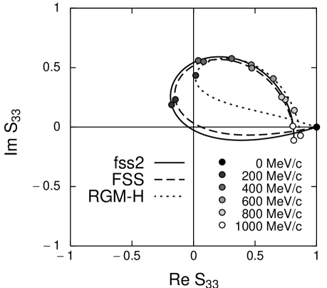
FIG. 17.: Argand diagram of the $S$-matrix element $S_{33}$ for the $\Lambda N$ - $\Sigma N(I=1/2)$ ${}^{3}S_{1}$ - ${}^{3}D_{1}$ coupled-channel system. The channel $i=3$ corresponds to the $\Sigma N(I=1/2)$ ${}^{3}S_{1}$ channel. The range of the incident momentum is $0\leq p_{\Sigma}\leq 1000$ MeV/$c$. Results given by fss2 (solid curve), FSS (dashed curve) and RGM-H (dotted curve) are displayed.

FIG. 18.: (a) The low-energy $\Sigma^{-}p$, $\Sigma^{0}n$ and $\Lambda n$ phase shifts for the ${}^{1}S_{0}$ channel, predicted by fss2, as a function of the incident momentum $p_{\Sigma}$. The solid curves include the full pion-Coulomb correction in the particle basis, while the dashed curves are obtained in the effective range approximation using the parameters in Table XIII. (b) $\Sigma^{-}p$ reflection and transmission coefficients $\mathchar 28945\relax_{i1}$ for the ${}^{1}S_{0}$ channel, predicted by fss2. The final channel $i$ is specified by 1: $\Sigma^{-}p$, 2: $\Sigma^{0}n$ and 3: $\Lambda n$. The solid curves denote the full calculation, while the dashed curves the effective range approximation.

FIG. 19.: (a) $\Sigma^{-}p$, $\Sigma^{0}n$ and $\Lambda n$ phase shifts for the ${}^{3}S_{1}+{}^{3}D_{1}$ state, predicted by fss2, as a function of the incident momentum $p_{\Sigma}$. $\Sigma^{-}p$ ${}^{3}D_{1}$ phase shift is not shown, since it is smaller than $0.1^{\circ}$. The full pion-Coulomb correction is included in the solid curves. The dashed curves are obtained in the effective range approximation using the parameters in Table XIV. (b) $\Sigma^{-}p$ reflection and transmission coefficients $\mathchar 28945\relax_{i1}$ for the ${}^{3}S_{1}+{}^{3}D_{1}$ channel, predicted by fss2. The final channel $i$ is specified by 1: $\Sigma^{-}p$ ${}^{3}S_{1}$, 2: $\Sigma^{-}p$ ${}^{3}D_{1}$, 3: $\Sigma^{0}n$ ${}^{3}S_{1}$, 4: $\Sigma^{0}n$ ${}^{3}D_{1}$, 5: $\Lambda n$ ${}^{3}S_{1}$ and 6: $\Lambda n$ ${}^{3}D_{1}$. $\mathchar 28945\relax_{21}$ and $\mathchar 28945\relax_{41}$ are not shown, since they are very small. The solid curves include the full pion-Coulomb correction, while the dashed curves are obtained in the effective range approximation.

FIG. 20.: $\Sigma^{-}p$ inelastic capture ratio in flight $r_{F}$, predicted by fss2, as a function of the incident momentum $p_{\Sigma}$. Calculation is made in the particle basis with (solid curve) and without (dashed curve) the Coulomb force.

FIG. 21.: Calculated low-energy of $\Sigma^{+}p$ and $\Sigma^{-}p$ scattering total cross sections by fss2 (solid curves), compared with experimental data: (a) $\Sigma^{+}p$ elastic, (b) $\Sigma^{-}p$ elastic, (c) $\Sigma^{-}p\rightarrow\Sigma^{0}n$ charge-exchange, (d) $\Sigma^{-}p\rightarrow\Lambda n$ reaction cross sections. Predictions in the particle basis without the Coulomb force (dashed curves), and those in the isospin basis (dotted curves) are also shown. The experimental data are taken from [53] for (a) and (b), and from [52] for (c) and (d).

FIG. 22.: Calculated $\Sigma^{+}p$ and $\Sigma^{-}p$ differential cross sections by fss2, compared with the experimental angular distributions: (a) $\Sigma^{+}p$ elastic scattering at $p_{\Sigma}=170~{}\hbox{MeV}/c$, (b) the same as (a) but at $p_{\Sigma}=450~{}\hbox{MeV}/c$, (c) $\Sigma^{-}p$ elastic scattering at $p_{\Sigma}=160~{}\hbox{MeV}/c$, (d) The same as (c) but at $p_{\Sigma}=550~{}\hbox{MeV}/c$, (e) $\Sigma^{-}p$ $\rightarrow$ $\Lambda n$ differential cross sections at $p_{\Sigma}=160~{}\hbox{MeV}/c$. The experimental data are taken from [52] for (a), [54] for (b), [53] for (c) and (e), and [55] for (d).

FIG. 23.: Calculated $NN$ and $YN$ total cross sections by fss2, compared with the experimental data. The solid curves denote the full calculation and the dotted curves the calculation in the isospin basis. The experimental data are taken from [9] for $NN$, [43], [44], [45] for $\Lambda p$, [52] for $\Sigma^{+}p$, and [53], [51], [55] for $\Sigma^{-}p$ scattering.

FIG. 24.: Nuclear matter saturation curves obtained for fss2 and FSS, together with the results of the Paris potential [56] and the Bonn model-B (Bonn-B) potential [31]. The choice of the intermediate spectra is specified by ”QTQ” and ”cont.”, respectively. The result for the Bonn-B potential in the continuous choice is taken from the non-relativistic calculation in [57].

FIG. 25.: (a) The nucleon s.p. potential $U_{N}(q_{1})$ in nuclear matter in the continuous choice for intermediate spectra. Predictions by fss2 for three densities $\mathchar 28954\relax=0.5\,\mathchar 28954\relax_{0},~{}0.7\,\mathchar 28954\relax_{0}$ and $\mathchar 28954\relax_{0}$ are shown. Here the normal density $\mathchar 28954\relax_{0}$ corresponds to $k_{F}=1.35~{}\hbox{fm}^{-1}$. The dashed curve is the result achieved by Schulze et al. [59] with the Nijmegen soft-core $NN$ potential NSC89 [58]. (b) The same as (a) but for the $\Lambda$ s.p. potential $U_{\Lambda}(q_{1})$. (c) The same as (a) but for the $\Sigma$ s.p. potential $U_{\Sigma}(q_{1})$. (d) The same as (a) but for the imaginary part of the $\Lambda$ and $\Sigma$ s.p. potentials $U_{B}(q_{1})$ predicted by fss2.

REFERENCES

- [1] Y. Fujiwara, C. Nakamoto, and Y. Suzuki, Prog. Theor. Phys. 94, 215 (1995).
- [2] Y. Fujiwara, C. Nakamoto, and Y. Suzuki, Prog. Theor. Phys. 94, 353 (1995).
- [3] Y. Fujiwara, C. Nakamoto, and Y. Suzuki, Phys. Rev. Lett. 76, 2242 (1996).
- [4] Y. Fujiwara, C. Nakamoto, and Y. Suzuki, Phys. Rev. C54, 2180 (1996).
- [5] T. Fujita, Y. Fujiwara, C. Nakamoto, and Y. Suzuki, Prog. Theor. Phys. 100, 931 (1998).
- [6] M. Kohno, Y. Fujiwara, T. Fujita, C. Nakamoto, and Y. Suzuki, Nucl. Phys. A674, 229 (2000).
- [7] Y. Fujiwara, M. Kohno, C. Nakamoto, and Y. Suzuki, Prog. Theor. Phys. 103, 755 (2000).
- [8] R. A. Bryan and B. L. Scott, Phys. Rev. 164, 1215 (1967).
- [9] R. A. Arndt, Scattering Analysis Interactive Dial-up (SAID), Virginia Polytechnic Institute, Blacksburg, Virginia (private communication).
- [10] Y. Fujiwara, M. Kohno, T. Fujita, C. Nakamoto, and Y. Suzuki, Nucl. Phys. A674, 493 (2000).
- [11] R. Machleidt, nucl-th/0006014 (2000).
- [12] M. Jurič et al., Nucl. Phys. B52, 1 (1973).
- [13] M. M. Nagels, T. A. Rijken, and J. J. de Swart, Ann. Phys. (N.Y.) 79, 338 (1973).
- [14] Y. Fujiwara, M. Kohno, C. Nakamoto, and Y. Suzuki, Prog. Theor. Phys. 104, 1025 (2000).
- [15] C. Nakamoto, Y. Suzuki, and Y. Fujiwara, Prog. Theor. Phys. 94, 65 (1995).
- [16] H. P. Noyes, Phys. Rev. Lett. 15, 538 (1965).
- [17] K. L. Kowalski, Phys. Rev. Lett. 15, 798, 908 (E) (1965).
- [18] Y. Fujiwara, Prog. Theor. Phys. 88, 933 (1992).
- [19] Y. Fujiwara, C. Nakamoto, Y. Suzuki, and Zhang Zong-ye, Prog. Theor. Phys. 97, 587 (1997).
- [20] K. Yazaki, Prog. Part. Nucl. Phys. 24, 353 (1990).
- [21] Zong-ye Zhang, Amand Faessler, U. Straub, and L. Ya. Glozman, Nucl. Phys. A578, 573 (1994).
- [22] T. Hamada and I. D. Johnston, Nucl. Phys. 34, 382 (1962).
- [23] V. G. J. Stoks, R. A. M. Klomp, C. P. F. Terheggen, and J. J. de Swart, Phys. Rev. C49, 2950 (1994).
- [24] K. Miyagawa and H. Yamamura, Phys. Rev. C60, 024003 (1999).
- [25] S. Shinmura, Y. Akaishi, and H. Tanaka, Prog. Theor. Phys. 71, 546 (1983).
- [26] Y. Yamamoto, T. Motoba, H. Himeno, K. Ikeda, and S. Nagata, Prog. Theor. Phys. Suppl. No. 117, 361 (1994).
- [27] E. Hiyama, Nucl. Phys. A670, 273c (2000).
- [28] H. Nemura, Y. Suzuki, Y. Fujiwara, and C. Nakamoto, Prog. Theor. Phys. 103, 929 (2000).
- [29] C. M. Vincent and S. C. Phatak, Phys. Rev. C10, 391 (1974).
- [30] Particle Data Group, Eur. Phys. J. C3, 1 (1998).
- [31] R. Machleidt, Adv. Nucl. Part. Phys. 19, 189 (1989).
- [32] O. Dumbrajs, R. Koch, H. Pilkuhn, G. C. Oades, H. Behrens, J. J. de Swart and P. Kroll, Nucl. Phys. B216, 277 (1983).
- [33] L. J. Allen, H. Fiedeldey, and N. J. McGurk, J. Phys. G4, 353 (1978).
- [34] M. Kohno, J. Phys. G9, L85 (1983).
- [35] N. L. Rodning and L. D. Knutson, Phys. Rev. C 41, 898 (1990).
- [36] David M. Bishop and Lap M. Cheung, Phys. Rev. A 20, 381 (1979).
- [37] G. A. Miller, M. K. Nefkens, and I. Slaus, Phys. Rep. 194,1 (1990).
- [38] C. R. Howell et al., Phys. Lett. B444, 252 (1998).
- [39] D. E. González Trotter et al., Phys. Rev. Lett. 83, 3788 (1999).
- [40] J. R. Bergervoet, P. C. van Campen, W. A. van der Sanden, and J. J. de Swart, Phys. Rev. C38, 15 (1988).
- [41] M. M. Nagels, T. A. Rijken, and J. J. de Swart, Phys. Rev. D12, 744 (1975).
- [42] T. Fujita, Y. Fujiwara, C. Nakamoto, and Y. Suzuki, Prog. Theor. Phys. 96, 65 (1996).
- [43] G. Alexander, U. Karshon, A. Shapira, G. Yekutieli, R. Engelmann, H. Filthuth, and W. Lughofer, Phys. Rev. 173, 1452 (1968).
- [44] B. Sechi-Zorn, B. Kehoe, J. Twitty, and R. A. Burnstein, Phys. Rev. 175, 1735 (1968).
- [45] J. A. Kadyk, G. Alexander, J. H. Chan, P. Gaposchkin, and G. H. Trilling, Nucl. Phys. B27, 13 (1971).
- [46] R. H. Dalitz, R. C. Herndon, and Y. C. Tang, Nucl. Phys. B47, 109 (1972).
- [47] Y. Fujiwara, T. Fujita, C. Nakamoto, and Y. Suzuki, Prog. Theor. Phys. 100, 957 (1998).
- [48] J. J. de Swart and C. Dullemond, Ann. Phys. 19, 458 (1962).
- [49] R. R. Ross, Bull. Ann. Phys. Sic. 3, 335 (1958).
- [50] V. Hepp and H. Schleich, Z. Phys. 214, 71 (1968).
- [51] D. Stephen, Ph. D. thesis, Univ. of Massachusetts, 1970 (unpublished).
- [52] R. Engelmann, H. Filthuth, V. Hepp, and E. Kluge, Phys. Lett. 21, 587 (1966).
- [53] F. Eisele, H. Filthuth, W. Föhlisch, V. Hepp, and G. Zech, Phys. Lett. 37B, 204 (1971).
- [54] J. K. Ahn et al., Nucl. Phys. A648, 263 (1999).
- [55] Y. Kondo et al., Nucl. Phys. A676, 371 (2000).
- [56] M. Lacombe, B. Loiseau, J. Richard, R. Vinh Mau, J. Côté, P. Pirès, and R. de Tourreil, Phys. Rev. C21, 861 (1980).
- [57] R. Brockmann and R. Machleidt, Phys. Rev. C42, 1965 (1990).
- [58] P. Maessen, Th. A. Rijken, and J. de Swart, Phys. Rev. C40, 2226 (1989).
- [59] H.-J. Schulze, M. Baldo, U. Lombardo, J. Cugnon, and A. Lejeune, Phys. Rev. C57, 704 (1998).
- [60] J. Dabrowski, Phys. Rev. C60, 025205 (1999).
- [61] R. Sawafta, Nucl. Phys. A585, 103c (1995); A639, 103c (1998).
- [62] H. Tamura, private communication from BNL E930 experiment (1999).
- [63] E. Hiyama, M. Kamimura, T. Motoba, T. Yamada, and Y. Yamamoto, Phys. Rev. Lett. 85, 270 (2000).
- [64] R. R. Scheerbaum, Nucl. Phys. A257, 77 (1976).
- [65] H. Bando, T. Motoba, and J. Z̆ofka, Int. J. of Mod. Phys. A21, 4021 (1990).
- [66] C. Nakamoto, Y. Suzuki, and Y. Fujiwara, Prog. Theor. Phys. 97, 761 (1997).
- [67] Y. Fujiwara and Y. C. Tang, Memoirs of the Faculty of Science, Kyoto University, Series A of Physics, Astrophysics, Geophysics and Chemistry, Vol. XXXIX, No. 1, Article 5, 91 (1994).
- [68] Y. Fujiwara and K. T. Hecht, Nucl. Phys. A462, 621 (1987).
- [69] M. Lacombe, B. Loiseau, J. Richard, R. Vinh Mau, J. Côté, P. Pirès, and R. de Tourreil, Phys. Lett. B101, 139 (1981).