Nuclear isotope shifts within
the local energy-density functional approach

Abstract

The foundation of the local energy-density functional method to describe the nuclear ground-state properties is given. The method is used to investigate differential observables such as the odd-even mass differences and odd-even effects in charge radii. For a few isotope chains of spherical nuclei, the calculations are performed with an exact treatment of the Gor’kov equations in the coordinate-space representation. A zero-range cutoff density-dependent pairing interaction with a density-gradient term is used. The evolution of charge radii and nucleon separation energies is reproduced reasonably well including kinks at magic neutron numbers and sizes of staggering. It is shown that the density-dependent pairing may also induce sizeable staggering and kinks in the evolution of the mean energies of multipole excitations. The results are compared with the conventional mean field Skyrme–HFB and relativistic Hartree–BCS calculations. With the formulated approach, an extrapolation from the pairing properties of finite nuclei to pairing in infinite matter is considered, and the dilute limit near the critical point, at which the regime changes from weak to strong pairing, is discussed.

PACS: 21.60.-n; 21.65.+f; 21.90.+f; 24.10.Cn

Keywords: Local energy-density functional; isotope shifts; staggering effects in nuclear properties; effective pairing interaction; sum rules; superfluid nuclear matter; dilute limit

, , ,

1 Introduction

For a long time, the fine structure of the isotopic dependence, i.e. dependence on the neutron number, of nuclear charge radii could not be explained satisfactorily. Because of the apparent lack of relevant experimental information, the effective particle–particle (pp) force which leads to the observed pairing properties of nuclei, has mostly been assumed in a very simple form, just sufficient to produce reasonable gap parameters $\bar{\Delta}$ extracted from the observed odd-even staggering in the nucleon separation energies. Even more sophisticated effective interactions, e.g. the Gogny force [1, 2, 3], do not include a density dependence in the pp channel.

It then has been demonstrated in Hartree-Fock-Bogolyubov (HFB) type calculations that three- or four-body forces are essential to reproduce the experimental data on isotope shifts of nuclear charge radii [4, 5, 6], and indeed that these isotope shifts give indirect experimental information on the effective in-medium many-body force, or what is equivalent, on the density dependence of the effective interaction, particularly in the pp channel.

It should be emphasized that a better knowledge of the density dependence of the nuclear pairing force would give the possibility to predict the pairing gap as a function of nuclear matter density which is, in particular, of great importance for understanding the pairing phenomena in neutron stars. It is well known that at present the pairing gap can not be obtained with sufficient accuracy from nuclear matter calculations based on bare NN interaction. The empirical information gained from the studies of real nuclei, specifically from the combined analyses of the nucleon separation energies and isotope shifts in charge radii, seems to be indispensable in this respect. A more general remark is that, as one may notice, a “good” microscopic theory, which could supply an effective interaction for describing the nuclear ground states and low-energy nuclear structure on a satisfactory level, is still lacking. The presently most successful simultaneous description of the bulk nuclear properties, such as binding energies and radii, throughout the periodic chart is achieved with phenomenological density-dependent interaction such as the Skyrme force [7]. This can be traced to the fact that some major effects produced by the density dependence of the effective interaction in the particle–hole (ph) channel, which is the second variational derivative of the corresponding energy-density functional with respect to normal density, are now established fairly well. On the same ground, one expects that simultaneous description of the differential observables, such as odd-even mass differences and the odd-even effects in radii, would shed light on the density dependence of the effective interaction in the pp channel.

In [4, 5, 6] an effective interaction has been chosen which consisted of two- and three- (or four-) body parts, with parameters adjusted independently of those of the single-particle potential used for the shell model description of the reference nucleus. Only differences with respect of this reference nucleus have been calculated in a self-consistent way.

This procedure corresponds to the philosophy of the Landau-Migdal theory of finite Fermi systems [10], where there is no simple connection between the single particle well parameters and the effective interaction of quasiparticles close to the Fermi surface. However, there are consistency requirements [11, 12, 13, 14, 15, 16] and since the parameters have been fitted to a large number of data, a quite reliable set of force parameters is available [16]. The interaction of Refs. [5, 6] has been restricted by the requirement that it should reduce to the Migdal force in the ph channel, the three-body part leading to the density dependence.

In the meantime, since Migdal had formulated his theory of finite Fermi systems (FFS), there has been much progress in Hartree-Fock calculations [17, 18, 19, 3], as well as in the self-consistent version of the FFS theory [15, 20, 16], demonstrating that initially Migdal may have been too pessimistic concerning the possibility to use the same interaction for ground state properties and for low-lying excited states.

In deriving the HF or HFB equations, the starting point is the minimization of the expectation value of the energy, expressed by an effective interaction. The latter is considered as a substitute for the $G$-matrix derived from the true NN interaction, appearing in some kind of “effective Hamiltonian”. Therefore, ideally, the same interaction should be used in the pp (hh) and the particle-hole (ph) channel. The energy is then obtained from the interaction and the state vector which is assumed to be a Slater determinant.

The self-consistent FFS theory or energy density functional (EDF) method starts from relations between the total energy, expressed as a functional of the density, the single particle potential, the effective interaction, and the quasiparticle density: Instead of parameterizing the interaction and deriving the energy from it in a certain approximation, an ansatz for the energy functional is assumed from which the other quantities can be derived. The interaction in the pp (hh) channel is obtained from the energy functional by a different procedure than that in the ph channel, and therefore these two interactions are different, which is of great practical importance. This feature is shared with Migdal’s theory of finite Fermi systems.

Otherwise, from a technical point of view, there is little difference between the EDF method and the HF or, with pairing, HFB method. The latter correspond to special choices of the energy functional. On the other hand in the EDF method, to compute the density, a Slater determinant or HFB-type state vector is employed. Thus the differences which exist in principle, due to the necessary approximations are of little practical importance.

In a recent paper [21] the EDF method has been applied to magic nuclei ^40,48Ca and ²⁰⁸Pb, investigating especially the influence of the spin–orbit interaction on collective states. Besides demonstrating the importance of including the two-body spin orbit force for the consistency of the method in describing the excited states, with the chosen set of parameters good results on the ground state properties have been obtained.

Here an analogous EDF approach is applied to open-shell nuclei with special attention to the pairing part of the functional. First results obtained mainly in diagonal-pairing approximation (i.e. with a HF–BCS formalism) have already been given in a few short publications [22, 23, 24] (the paper [23] gives the first application of the EDF approach to deformed nuclei and contains the results of a HFB-type calculation for dysprosium isotopes). In the present paper we give the results of more elaborate calculations based on the coordinate-space technique developed in [25] which allows us, for a local pairing field $\Delta(\vec{r})$, to solve the Gor’kov equations in spherical finite systems without any approximations [26]. The latter approach, even in the case of contact pairing force, corresponds, to a good approximation as will be shown in the present paper, to a full treatment of the HFB problem by applying the general variational principle to the EDF with a fixed energy cutoff $\epsilon_{\rm c}>\epsilon_{\rm F}$ ($\epsilon_{\rm F}$ is the Fermi energy). It is known from nuclear matter calculations that $s$-wave pairing vanishes at or slightly above the equilibrium density $\approx 0.16$ fm^-3; and so, in our local EDF approach, the cutoff is chosen to be larger than the corresponding Fermi energy $\epsilon_{0\rm F}\approx 37$ MeV. In actual calculations we shall use $\epsilon_{\rm c}=40$ MeV.

In Section 2 we give some theoretical foundation of the local EDF method for superfluid nuclei. In Section 3 the normal part of the energy-density functional with the parameters used in the calculations is described. In Section 4 the pairing part of the functional is presented. There, a possible extrapolation to uniform nuclear matter and the dilute limit with weak and strong pairing is also considered. Section 5 is devoted to the analysis of specific numerical results for a few isotopic chains of spherical nuclei and to the comparison of these results with experimental observations and other theoretical approaches. The influence of the density-dependent pairing on the evolution of the mean energies of multipole excitations is also studied using the self-consistent sum rule approach. In Section 6, the contribution of the ground state (“phonon”) correlations to the charge radii is analyzed. In Section 7 the conclusions are summarized. Some important theoretical and technical aspects are presented in the Appendices A, B, and C. Appendix A contains a thorough formulation of the generalized variational principle for the systems with pairing correlations which could be described by a local cutoff EDF. In Appendix B, the expression for the pairing energy is derived by using the Green’s function formalism. In Appendix C, we give a detailed description of the coordinate-space technique which we apply here to spherical nuclei.

2 Method of the local energy functional with pairing

In this section we give some foundation of the local-energy-density functional method which we apply here. Let us first briefly mention a few approaches used to calculate the nuclear ground state energy which is the expectation value of the Hamiltonian $\hat{H}$ (with a “bare” NN-interaction) over the exact ground state vector $|\Phi\rangle$:

$$E=\langle\Phi|{\hat{H}}|\Phi\rangle\,.$$ (2.1)

In general, the vector $|\Phi\rangle$ is a functional of the particle density $\varrho^{\rm p}$ [27] given by

$$\varrho^{\rm p}(\vec{r}_{1})={\rm Tr}_{st}\langle\Phi|\Psi^{\dagger}(1)\Psi(1)|\Phi\rangle\,,$$ (2.2)

where $s$ and $t$ are the spin and isospin indices and $\Psi^{\dagger}(1)$ and $\Psi(1)$ are the particle creation and annihilation operators, respectively, $(1)=(\{\vec{r},s_{z},\tau_{3}\}_{1})$. Therefore, the energy is a functional of $\varrho^{\rm p}$:

$$E=E[\varrho^{\rm p}]\,.$$

It is a difficult problem to construct such a functional and calculate the energy for many body systems. Formally, one can introduce single-particle degrees of freedom and, assuming that there is no pairing condensate, extract the single-particle motion on the HF level by writing

$$E[\hat{\rho}]=\langle{\rm HF}|{\hat{H}}|{\rm HF}\rangle+E_{\rm corr}[\hat{\rho}]\,,$$ (2.3)

where $|{\rm HF}\rangle$ is the HF vacuum — a Slater determinant of single-particle wave functions $\phi_{i}$. The latter are defined in a self-consistent manner by the equation $\hat{h}\phi_{i}=\epsilon_{i}\phi_{i}$ in which the single-particle Hamiltonian $\hat{h}$ is given by the variational derivative of the energy functional with respect to the single-particle density matrix $\hat{\rho}$: $\hat{h}=\delta E/\delta\hat{\rho}$. The second term, $E_{\rm corr}$, is the dynamical correlation energy (short range correlations, RPA correlations, many-particle correlations, parquet diagrams, etc.). The density matrix $\hat{\rho}$ may be associated with the Landau-Migdal quasiparticle density matrix defined as

$$\hat{\rho}(1,2)=\langle{\rm HF}|\psi^{\dagger}(2)\psi(1)|{\rm HF}\rangle\,,$$

with $\psi^{\dagger}$ ($\psi$) the quasiparticle creation (annihilation) operators. It is in turn a functional of the particle density $\varrho^{\rm p}$:

$$\hat{\rho}=\hat{\rho}[\varrho^{\rm p}]\,.$$

In homogeneous infinite nuclear matter, because of equality of the particle and quasiparticle numbers, the following relation between the two densities holds:

$$\varrho^{\rm p}=\rho={\rm Tr}_{st}\hat{\rho}(1,1)\,.$$ (2.4)

In an inhomogeneous system, the local difference between the densities could be attributed to the quasiparticle form factor [15]. Using the effective radius approximation one may write

$$\varrho^{\rm p}(\vec{r})=(1+\textstyle{\frac{1}{6}}R^{2}_{\rm q}{\vec{\nabla}}^{2})\rho(\vec{r})\,,$$ (2.5)

where $R_{\rm q}$ is the effective quasiparticle radius.

Hence the mean square nuclear radius for the particles may differ from that for the quasiparticles:

$$\langle r^{2}\rangle^{\rm p}=\langle r^{2}\rangle+R^{2}_{\rm q}\,.$$ (2.6)

Some additional effects may be related with a possible change of the internal structure of nucleons in nuclear medium. Such effects are not included explicitly in the ordinary approaches, based either on a “bare” Hamiltonian $H$ or on some kind of effective interaction, in which the nucleons or quasiparticles are considered as point-like objects. Within the EDF approach, however, tracing back to the Hohenberg–Kohn density-functional theory [27], if the functional were known, its minimization would determine both the ground-state energy and the correct particle density $\varrho^{\rm p}(\vec{r})$. Anyway, for the differences between mean square radii of nuclei, which is of our main interest here, one has

$$\delta\langle r^{2}\rangle^{\rm p}=\delta\langle r^{2}\rangle\,.$$ (2.7)

The common problem of any many-body theory is how to calculate the dynamical correlation energy $E_{\rm corr}$ or how to take it into account in some effective way. In nuclear physics a few self-consistent methods are very popular:

• The HF method with effective density-dependent interaction (e.g., with zero-range Skyrme [19] or finite-range Gogny force [3]). In this method the energy is calculated as a ground state expectation value of an effective Hamiltonian $H_{\rm eff}$ taken over a Slater determinant,

  $$E[\hat{\rho}]=\langle{\rm HF}|{\hat{H}}_{\rm eff}|{\rm HF}\rangle\,.$$ (2.8)

• The relativistic mean field model [29, 30] based on a phenomenological relativistic Lagrangian which includes mesonic and nucleonic degrees of freedom. In most applications to the ground states of finite nuclei, the relativistic Hartree formalism with static meson fields, and with no-sea approximation for nucleons, has been used (see [31] and references therein).

• The quasiparticle Lagrangian method (QLM) which is an extension [15] of the Landau-Migdal quasiparticle concept. In this method an effective local quasiparticle Lagrangian is constructed taking into account the first-order energy-dependence of the nucleon mass operator and the requirements imposed by self-consistency relations [13]. The QLM can be reformulated in terms of an effective Hamiltonian [32] in which the (linear) energy dependence of the nucleon mass operator is completely hidden so that this approach becomes equivalent to the EDF method (see also the discussion of this point in [20]).

• The method of the effective quasiparticle local energy density functional (which is referred to as EDF here). The possibility to use this method is based on the existence theorem of Hohenberg and Kohn [27]. With the Kohn-Sham quasiparticle formalism [33], this theorem allows one to write the nuclear EDF in the form

  $$E[\hat{\rho}]={\rm Tr}(t\hat{\rho})+E_{\rm int}[\rho]\,,$$ (2.9)

  where the first term is taken with the free kinetic energy operator $t=p^{2}/2m$ ($m$ is the bare nucleon mass). The ground state energy is then determined by making this EDF stationary with respect to infinitesimal variations of the single-particle wave functions belonging to the class of the Slater determinants from which the density matrix $\hat{\rho}$ (and the density $\rho$) can be calculated self-consistently. This method is flexible in the sense that the EDF does not (and should not) expose the same symmetry properties for the effective force, which is the second variational derivative of the EDF with respect to $\rho$, as the underlying bare NN interaction or effective Skyrme-type forces. Particularly, the force in the ph channel obtained from the EDF does not come out to be antisymmetrized, and the effective force in the pp channel needed for describing the nuclear pairing properties has to be derived in a different way. As a result, the matrix elements of the pp force, although they should be antisymmetrized, have no direct connection, say by means of simple angular momentum recoupling like the Pandya transformation, with those of the ph force. This is, as discussed in the Introduction, in accord with the philosophy of Migdal theory of finite Fermi systems [10]. (For an example of the phenomenological nuclear EDF see [20, 21]).

In most of the applications of the conventional functionals to finite nuclei the pairing correlations are introduced either at the BCS or the HFB level (see, e.g., Ref. [37] and references therein). When the contact pairing interaction is used, the pairing part of the functional is usually evaluated within a truncated space of the quasiparticle levels imposing an energy cutoff which is often chosen with some freedom but not too far from the Fermi surface. A more rigorous approach should be based on the general variational principle for the cutoff functional which uses the same quasiparticle basis both in the ph and pp channel.

We proceed as follows. In nuclei with pairing correlations one works with approximate state vectors which are not eigenstates of the particle number. One assumes nonzero anomalous expectation values, ${\hat{\nu}}(1,2)=\langle\Phi|\Psi(1)\Psi(2)|\Phi\rangle\neq 0$, and the energy of a superfluid nucleus may be given by a functional of the generalized density matrix $\widehat{R}$ containing both normal, $\hat{\rho}$, and anomalous, $\hat{\nu}$, components (see Appendix A). In analogy to eq. (2.3), the energy of a superfluid nucleus can be written as

$$E[\widehat{R}]=\langle{\rm HFB}|{\widehat{H}}|{\rm HFB}\rangle+E_{\rm corr}[\widehat{R}]\,$$ (2.10)

with $|{\rm HFB}\rangle$ the HFB quasiparticle vacuum and $E_{\rm corr}$ the dynamical correlation energy.

The generalized density matrix $\widehat{R}$, in turn, is a functional of $\varrho^{\rm p}$ and therefore

$$E=E[\widehat{R}[\varrho^{\rm p}]]=E[\varrho^{\rm p}]\,.$$ (2.11)

The method we follow here is based on an effective quasiparticle energy functional of the generalized density matrix:

$$E[\widehat{R}]=E_{\rm kin}[{\hat{\rho}}]+E_{\rm int}[{\hat{\rho}},{\hat{\nu}}]\,,$$ (2.12)

where $E_{\rm kin}[{\hat{\rho}}]={\rm Tr}(t\hat{\rho})\,,$ and $E_{\rm int}[{\hat{\rho}},{\hat{\nu}}]=E_{\rm int(normal)}[{\hat{\rho}}]+E_{\rm anomal}[{\hat{\rho}},{\hat{\nu}}]\,.$ The anomalous energy $E_{\rm anomal}$ is chosen such that it vanishes in the limit $\nu\to 0$.

It should be emphasized that the weak-pairing approximation $|\bar{\Delta}|\ll\epsilon_{\rm F}$ is assumed throughout this paper. That means we need to retain only the first-order term $\sim\nu^{2}$ in the $\nu$-dependent, anomalous part of the energy functional. One may then write

$$E_{\rm anomal}[{\hat{\rho}},{\hat{\nu}}]={\textstyle\frac{1}{4}}\left({\hat{\nu}}^{\dagger}{\hat{\mathcal{F}}}^{\rm pp}_{\rm a}[{\hat{\rho}}]{\hat{\nu}}\right)\,,$$ (2.13)

where ${\hat{\mathcal{F}}}^{\rm pp}_{\rm a}$ is an antisymmetrized effective interaction in the pp channel and the round brackets (…) imply integration and summation over all variables.

To calculate the ground state properties, one can now use the general variational principle with two constraints,

$$\langle{\rm HFB}|{\hat{N}(\mu)}|{\rm HFB}\rangle\equiv N(\mu)=N\,,$$ (2.14)

$${\widehat{R}}^{2}=\widehat{R}\,,$$ (2.15)

leading to the variational functional of the form

$$I[\widehat{R}]=E[\widehat{R}]-\mu N(\mu)-{\rm Tr}{\hat{\Lambda}}(\widehat{R}-{\widehat{R}}^{2})\,,$$ (2.16)

where $N$ is the particle number, $\mu$ the chemical potential, and ${\hat{\Lambda}}$ the matrix of Lagrange parameters (see, e.g. Ref. [28], and Appendix A for more details).

The major difficulty in implementing this general variational principle in practice is connected with the anomalous part of the energy functional. The anomalous energy (2.13) can be calculated if one knows a solution of the gap equation for the pairing field $\hat{\Delta}$ and the anomalous density matrix $\hat{\nu}$. In general, the gap equation,

$$\hat{\Delta}={\textstyle\frac{1}{2}}{\hat{\mathcal{F}}}^{\rm pp}_{\rm a}{\hat{\nu}}\,,$$ (2.17)

is nonlocal and its solution (starting, for example, from a realistic bare NN interaction [38, 39, 40, 41]), even for uniform nuclear matter, poses serious problems. First attempts were made very recently to construct an effective pairing interaction for semi-infinite nuclear matter [42] and for finite nuclei [43] with an approximate version of the Brueckner approach. Those studies are in an initial stage, and so far they do not give any guidance how to choose an effective pairing interaction, in particular its density dependence, that could be used in nuclear structure calculations. It is assumed that a simple universal effective interaction in the pp-channel can be invented to correctly describe the nuclear pairing properties. Our intention is to show that, to a good approximation in the case of weak pairing $|\bar{\Delta}|\ll\epsilon_{\rm F}$, the EDF method and the general variational principle can be used with an effective density-dependent contact pp-interaction.

We proceed with the formal development by using the Green’s function formalism as described in detail in Appendices A and B. Here we give only a brief account of the main issues.

We introduce an arbitrary cutoff $\epsilon_{\rm c}$ in the energy space, but such that $\epsilon_{\rm c}>\epsilon_{\rm F}$, and split the generalized density matrix into two parts,

$$\widehat{R}={\widehat{R}}_{\rm c}+\delta_{\rm c}{\widehat{R}}\,,$$ (2.18)

where $\delta_{\rm c}{\widehat{R}}$ is related to the integration over energies $|\epsilon|>\epsilon_{\rm c}$.

The gap equation is renormalized to yield

$$\hat{\Delta}={\textstyle\frac{1}{2}}\hat{\mathcal{F}}^{\xi}_{\rm a}{\hat{\nu}}_{\rm c}\,,$$ (2.19)

where ${\hat{\nu}}_{\rm c}$ is the cutoff anomalous density matrix and $\hat{\mathcal{F}}^{\xi}_{\rm a}$ is the effective antisymmetrized pp-interaction in which the contribution coming from the energy region $|\epsilon|>\epsilon_{\rm c}$ far from the Fermi surface is included by renormalization (see Appendix A).

For homogeneous infinite matter with weak pairing ($|\bar{\Delta}|\ll\epsilon_{\rm F}$), it is shown that the variational functional $E-\mu N$ does not change in first order in $|\bar{\Delta}|^{2}/\epsilon_{\rm F}$ upon variation with respect to $\delta_{\rm c}{\widehat{R}}$. The total energy of the system and the chemical potential also remain the same in first order in $|\bar{\Delta}|^{2}/\epsilon_{\rm F}$ if one imposes the particle number constraint (2.14) for the cutoff functional. To a good approximation, as discussed in Appendix A, this should also be valid for finite (heavy) nuclei.

Such an outcome may be understood by noting that the major pairing effects, if $|\bar{\Delta}|\ll\epsilon_{\rm F}$ which is generally the case in nuclear matter and in finite nuclei, are developed near the Fermi surface. In this connection we mention the well-known fact that the pairing energy, in the BCS approximation, is defined by a sum concentrated near the Fermi surface (see, for example, Ref. [28]):

$$E_{\rm pair}\approx-{\textstyle\frac{1}{2}}{\bar{n}}{\bar{\Delta}}^{2}\,,$$ (2.20)

with $\bar{n}$ the average level density and $\bar{\Delta}$ the average energy gap in the vicinity of the Fermi surface. In infinite matter, this corresponds to the pairing energy per particle (see Appendix B):

$$\frac{E_{\rm pair}}{N}=-\frac{3}{8}\frac{\Delta^{2}(\vec{p}_{\rm F})}{\epsilon_{\rm F}}\,.$$ (2.21)

It follows that, with the cutoff functional, this leading pairing contribution to the energy of the system is exactly accounted for.

Thus we find that nuclear ground state properties can be described by applying the general variational principle to minimize the cutoff functional which has exactly the same form as in eq. (2.16) with the constraint (2.14) but with $\widehat{R}$ replaced by $\widehat{R}_{\rm c}$:

$$I_{\rm c}[\widehat{R}]=E_{\rm kin}[{\hat{\rho}}_{\rm c}]+E^{\rm c}_{\rm int}[\rho_{\rm c},\nu_{\rm c}]-\mu_{\rm c}N_{\rm c}(\mu_{\rm c})-{\hat{\Lambda}}(\widehat{R}-{\widehat{R}}^{2})\,,$$ (2.22)

$$\langle{\rm HFB}|{\hat{N}_{\rm c}(\mu_{\rm c})}|{\rm HFB}\rangle\equiv N_{\rm c}(\mu_{\rm c})=N\,.$$ (2.23)

Here $E_{\rm kin}[{\hat{\rho}}_{\rm c}]={\rm Tr}(t{{\hat{\rho}}_{\rm c}})\,$ and $E^{\rm c}_{\rm int}[\rho_{\rm c},\nu_{\rm c}]=E^{\rm c}_{\rm int(normal)}[{\hat{\rho}}_{\rm c}]+E^{\rm c}_{\rm anomal}[{\hat{\rho}}_{\rm c},{\hat{\nu}}_{\rm c}]\,$ with

$$E^{\rm c}_{\rm anomal}[{\hat{\rho}_{\rm c}},{\hat{\nu}}_{\rm c}]={\textstyle\frac{1}{4}}({\hat{\nu}}^{\dagger}_{\rm c}{\hat{\mathcal{F}}}^{\xi}_{\rm a}[{\hat{\rho}}_{\rm c}]{\hat{\nu}}_{\rm c})\,.$$ (2.24)

The above consideration has been carried out without any pre-assumptions concerning the density functional $E_{\rm int}[\widehat{R}]\approx E^{\rm c}_{\rm int}[\rho_{\rm c},\nu_{\rm c}]\,$. Now, recalling the Hohenberg-Kohn theorem [27], we specify that the density functional can be chosen to be of a local form, i.e. dependent on the normal and anomalous local real densities $\rho(\vec{r},\tau)$ and $\nu(\vec{r},\tau)$ defined in Appendix A by (A.61) and (A.64), respectively. Then $E^{\rm c}_{\rm normal}$ is a functional of the normal densities (isoscalar, isovector, spin–orbital, etc.), and $E^{\rm c}_{\rm anomal}$ is a functional of the normal and anomalous densities, the latter acquiring the simple form

$$E^{\rm c}_{\rm anomal}[\rho_{\rm c},\nu_{\rm c}]=\sum_{\tau=\rm n,p}\int\d{\vec{r}}\,\nu^{*}_{\rm c}(\vec{r},\tau){\mathcal{F}}^{\xi}(\vec{r},\tau;[\rho_{\rm c}])\nu_{\rm c}(\vec{r},\tau)\,.$$ (2.25)

The pairing potential is defined by

$$\Delta(\vec{r},\tau)=\frac{1}{2}\frac{\delta E^{\rm c}_{\rm anomal}[\rho_{\rm c},\nu_{\rm c}]}{\delta\nu_{\rm c}(\vec{r},\tau)}\,.$$ (2.26)

That corresponds to the gap equation which takes on now a very simple multiplicative form:

$$\Delta(\vec{r},\tau)={\mathcal{F}}^{\xi}(\vec{r},\tau;[\rho_{\rm c}])\nu_{\rm c}(\vec{r},\tau)\,.$$ (2.27)

The normal mean-field potential is given by

$$U(\vec{r},\tau)=\frac{\delta E^{\rm c}_{\rm int}[\rho_{\rm c},\nu_{\rm c}]}{\delta\rho_{\rm c}(\vec{r},\tau)}\,.$$ (2.28)

Due to the density dependence of ${\mathcal{F}}^{\xi}$ it includes also a contribution arising from the variation of the pairing interaction energy:

$$U_{\rm pair}(\vec{r},\tau)=\frac{\delta E^{\rm c}_{\rm anomal}[\rho_{\rm c},\nu_{\rm c}]}{\delta\rho_{\rm c}(\vec{r},\tau)}\,.$$ (2.29)

We emphasize that having found the gap function $\Delta(\vec{r})$, and the mean-field potential $U(\vec{r})$, the Gor’kov equations [44] may be solved, for spherical nuclei, exactly by using the coordinate-space technique (see Refs. [25, 20, 26] and Appendix C). The generalized Green’s function obtained this way can be integrated over energy up to $\epsilon_{\rm c}$ to yield both the normal and anomalous densities $\rho_{\rm c}$ and $\nu_{c}$ which are used then to compute the energy of the system. This corresponds to a full HFB treatment of the nuclear ground state properties. It remains, of course, an art to find a “good” local functional, in particular its anomalous part.

3 The normal part of the functional

In this and the next section we describe in some detail the energy-density functional which we use in the present calculations. We shall omit in the following the cutoff index c for simplicity. The functional is local in the sense that it contains only normal and anomalous densities, not the density matrix. The interaction part of the energy density is

$$\varepsilon_{\rm{int}}=\varepsilon_{\rm{main}}+\varepsilon_{\rm{Coul}}+\varepsilon_{sl}+\varepsilon_{ss}+\varepsilon_{\rm anomal}\,.$$ (3.1)

The terms $\varepsilon_{\rm main}$ and $\varepsilon_{\rm Coul}$ have been described in Refs. [21, 45], where also the connection of the parameters involved with the characteristics of nuclear matter has been given. Two different versions of the spin–orbit part $\varepsilon_{sl}$ have been used: the one of Ref. [21], and also, after [20], the variant

$$\varepsilon_{sl}(\vec{r}) = {\frac{1}{2}}C_{0}r_{0}^{2}\sum_{i,k={\rm p,n}}\left\{\kappa^{ik}[\nabla\rho^{i}\cdot\sum_{ss^{\prime}}\langle\psi^{\dagger}(\vec{r},s)[\vec{p}\times\vec{\sigma}]\psi(\vec{r},s^{\prime})\rangle^{k}\right.$$ (3.2)

$$+ \nabla\rho^{k}\cdot\sum_{ss^{\prime}}\langle\psi^{\dagger}(\vec{r},s)[\vec{p}\times\vec{\sigma}]\psi(\vec{r},s^{\prime})\rangle^{i}]$$

$$+ \left.g_{1}^{ik}\sum_{\alpha,\beta}\sum_{ss^{\prime}}\langle\psi^{\dagger}(\vec{r},s)\sigma_{\alpha}p_{\beta}\psi(\vec{r},s^{\prime})\rangle^{i}\sum_{ss^{\prime}}\langle\psi^{\dagger}(\vec{r},s)\sigma_{\alpha}p_{\beta}\psi(\vec{r},s^{\prime})\rangle^{k}\right\}$$

where $\psi^{\dagger}$ and $\psi$ are field operators, the brackets denote the ground state expectation value, and a superscript $k$ indicates that a projection on particles of type $k$ is performed.

As given by (3.2), $\varepsilon_{sl}$ corresponds to the two-body spin–orbit interaction

$${\mathcal{F}}^{\omega}_{sl}=C_{0}r_{0}^{2}(\kappa+\kappa^{\prime}\vec{\tau}_{1}\!\cdot\!\vec{\tau}_{2})[\nabla_{1}\delta(\vec{r}_{1}-\vec{r}_{2})\times(\vec{p}_{1}-\vec{p}_{2})]\!\cdot\!(\vec{\sigma}_{1}+\vec{\sigma}_{2})\,,$$ (3.3)

and to the first–order velocity harmonic of the spin–dependent part of the Landau interaction amplitude

$${\mathcal{F}}^{\omega}_{1}=C_{0}r_{0}^{2}(g_{1}+g_{1}^{\prime}\vec{\tau}_{1}\!\cdot\!\vec{\tau}_{2})\delta(\vec{r}_{1}-\vec{r}_{2})(\vec{\sigma}_{1}\!\cdot\!\vec{\sigma}_{2})(\vec{p}_{1}\!\cdot\!\vec{p}_{2})\,,$$ (3.4)

which has to be symmetrized in such a way that the momentum operators ${\vec{p}}_{1,2}$ never act on the delta-function $\delta(\vec{r}_{1}-\vec{r}_{2})$.

In these expressions, the multiplier $r_{0}^{2}$ has been introduced to make the parameters $\kappa$ and $g_{1}$ dimensionless. It is given by $r^{2}_{0}=(3/8\pi\rho_{0})^{2/3}$ where $\rho_{0}$ is the equilibrium density of one kind of particles in symmetric nuclear matter. The factor $C_{0}$ is the inverse density of states at the Fermi energy, $\epsilon_{0\rm F}=k_{0\rm F}^{2}/2m^{*}$, in saturated nuclear matter. It is given by $C_{0}=2\epsilon_{0\rm F}/3\rho_{0}=\pi^{2}/k_{0\rm F}m^{*}$.

Defining spin–orbit densities by

$$\rho^{k}_{sl}(\vec{r})=\sum_{ss^{\prime}}\langle\psi^{\dagger}(\vec{r},s)({\vec{\sigma}}\!\cdot\!{\vec{l}})\psi(\vec{r},s^{\prime})\rangle^{k}\,,$$

then in spherically symmetric nuclei, the spin–orbit energy density (3.2) can be simplified to [20]

$$\varepsilon_{sl}=C_{0}r_{0}^{2}\sum_{i,k={\rm n,p}}\left({\frac{1}{r}}\rho_{sl}^{i}\kappa^{ik}{\frac{\partial\rho^{k}}{\partial r}}+{\frac{1}{4r^{2}}}\rho_{sl}^{i}g_{1}^{ik}\rho_{sl}^{k}\right)\,.$$ (3.5)

In deformed nuclei, the expression for $\varepsilon_{sl}$ cannot be written in such a simple form. In the axially symmetric case the derivation can be performed in cylindrical coordinates; the resulting formulae are given in [23].

We just mention some features of those parts of $\varepsilon_{\rm int}$ which are not given here in detail: The main contribution $\varepsilon_{\rm main}$ consists of a volume part and of a surface term both containing simple fractional-linear functions of the normal isoscalar density $\rho_{+}=\rho_{\rm n}+\rho_{\rm p}$. This leads to the effective density-dependent forces in the scalar-isoscalar and scalar-isovector channels (see e.g. Refs. [20, 21, 45] for more details). There is no momentum dependence in these parts, therefore we have the effective mass $m^{*}$ equal to the bare mass $m$. The surface term involves a finite, but small Yukawa range parameter $R=0.35$ fm; in the limit $R\rightarrow 0$ it could be written with the help of the Laplace operator acting on functions of the density. It vanishes for constant density. The Coulomb part $\varepsilon_{\rm Coul}$ is taken in the usual form [19] with an exchange contribution in the Slater approximation.

Note that in the more complicated parts of the force like those of eqs. (3.3) and (3.4) we did not introduce any density dependence. In general, all of the constants $\kappa$, $g_{1}$, and others to follow below could be density dependent as well. Until now there are no experimental data which would make it necessary to introduce such a dependence for the laboratory nuclei within or not too far from the stability valley. However, going to the nucleon drip lines and beyond, a more complicated density-dependent spin–orbit force might be of relevance. This is indicated by the relativistic mean field models for very neutron-rich nuclei [46] and by the exact Monte Carlo methods for small pure neutron drops [47]. Both approaches predict a much smaller (by a factor of 2–3) spin–orbit potential than the usual Skyrme-type ansatz. The role played by the density dependence of the effective spin–orbit interaction is left to be studied in future work.

The spin–spin term $\varepsilon_{ss}$ has hitherto been omitted since its expectation value in spin-zero nuclei vanishes. We include it here for completeness; it might become important for magnetic excitations or polarization. A possible simple form of it is

$$\varepsilon_{ss}(\vec{r})={\textstyle\frac{1}{2}}C_{0}\sum_{i,k={\rm n,p}}g_{0}^{ik}\langle\vec{\sigma}\rangle^{i}\!\cdot\!\langle\vec{\sigma}\rangle^{k}\,.$$ (3.6)

Note that the strength $\propto g_{0}^{ik}$ can be considered as the zeroth term in a decomposition of the spin–spin interaction amplitude at the Fermi surface in Legendre polynomials of the scattering angle. The next (first) term, proportional to $g_{1}^{ik}$, has been included in the spin–orbit part of the functional; however, the normalization chosen in eq. (3.2) is different from that of Ref. [10].

As long as there is no static spin polarization ($\langle\vec{\sigma}\rangle=0$) in the ground states of even nuclei and our interest is only in electric and mass quantities we can continue to neglect $\varepsilon_{ss}$. One delicate point should be addressed in this connection. Usually, when deriving the Hartree-Fock equations, one starts with a Hamiltonian containing a well behaved and properly antisymmetrized interaction. In the case of contact forces, antisymmetry prevents self-interaction of the particles, so there is no need for precautions against that. Going over to an effective force which, as in our case, is not antisymmetrized in the ph channel, the self-interaction is not automatically excluded. Dealing with a not-too-small number of particles, by fitting to the experimental data the self-interaction is compensated (or accounted for) in the average by the choice of the parameters.

This does not hold for the spin–spin part of the force. For an odd nucleus, consisting of a core with $J=0$ plus one particle, there is a nonvanishing spin density, and from eq. (3.6) there is also a contribution to the total energy which to lowest order is just the self-interaction of the odd particle and should therefore be excluded. On the other hand, considering the contribution of this part of the functional to the single particle potential when determining the wave function of the core, will give the polarization of the core which is a physical quantity. — Usually, on the level of Hartree-Fock type calculations the spin–spin interaction is left out; it may be considered in a second step by perturbation methods.

The basic set of functional parameters in the notations of Refs. [20, 21, 48] used in the present calculations is the set DF3:

$$\left.\begin{array}[]{ll}a^{\rm v}_{+}=-6.422,&a^{\rm v}_{-}=5.417,\\ h^{\rm v}_{1+}=0.163,\,\,h^{\rm v}_{2+}=0.724,&h^{\rm v}_{1-}=0,\,\,h^{\rm v}_{2-}=3.0,\\ a^{\rm s}_{+}=-11.1,\,\,h^{\rm s}_{+}=0.31,&a^{\rm s}_{-}=-4.00,\,\,h^{\rm s}_{-}=0,\\ \kappa^{\rm pp}=0.285,\,\,\kappa^{\rm pn}=0.135,&g_{1}^{\rm pp}=-g_{1}^{\rm pn}=-0.12,\\ r_{0}=1.147~{}{\rm fm},&R=0.35~{}{\rm fm}\,.\\ \end{array}\right\}$$ (3.7)

This set set has been specifically deduced in [48] to reproduce not only the already known ground-state properties of magic nuclei but also the very recent experimental data [49] on the single-particle energies near the “magic cross” at ¹³²Sn. The set (3.7) corresponds to the following nuclear matter characteristics at saturation: compression modulus $K_{0}=200$ MeV, chemical potential (binding energy per nucleon) $\mu_{0}=-16.05$ MeV, asymmetry energy parameter $\beta_{0}=28.7$ MeV, saturation density $2\rho_{0}=0.1582$ fm^-3 ($k_{0\rm F}=1.328$ fm^-1, $\epsilon_{0\rm F}=36.57$ MeV, $C_{0}=\pi^{2}/k_{0\rm F}m=308.2$ MeV$\cdot$fm³). As in Ref. [20], the functional contains zero-range isoscalar spin–orbit interaction $\propto\kappa$ and velocity-dependent spin-isospin interaction $\propto g_{1}^{\prime}$ (i.e. the first Landau-Migdal harmonic in the $\sigma\tau$ channel). This is in contrast to [21] where a finite range spin–orbit force had been used.

With the above parameter set of the normal part of the density functional the ground states of magic nuclei are described fairly well. For example, the calculated rms charge radii $\langle r^{2}_{\rm ch}\rangle^{1/2}$ of ⁴⁰Ca, ⁴⁸Ca and ²⁰⁸Pb are 3.480 fm, 3.478 fm, and 5.500 fm, respectively, which agree nicely with experimental values deduced very recently [50] from the combined analysis of optical, muonic and elastic electron scattering data: $\langle r^{2}_{\rm ch}\rangle^{1/2}=3.4767(8)$ fm for ⁴⁰Ca, 3.4736(8) fm for ⁴⁸Ca, and 5.5013(7) fm for ²⁰⁸Pb. The predictions for some other double magic nuclei are: $\langle r^{2}_{\rm ch}\rangle^{1/2}=3.721$ fm (⁵⁶Ni), 3.951 fm (⁷⁸Ni), 4.453 fm (¹⁰⁰Sn), and 4.705 fm (¹³²Sn).

4 The pairing part of the functional

The pairing energy density $\varepsilon_{\rm anomal}$ in eq. (3.1) is chosen in the form prescribed by (2.25):

$$\varepsilon_{\rm anomal}(\vec{r})=\sum_{\tau=n,p}{\mathcal{F}}^{\xi,\tau\tau}(\vec{r};[\rho])|\nu_{\tau}(\vec{r})|^{2}\,.$$ (4.1)

As discussed in Refs. [4, 5, 6] and mentioned in the introduction, effective three- or more-body forces are indispensable if one wants to reproduce isotope shifts in charge radii which means that $\varepsilon_{\rm anomal}$ must depend on the normal density [22, 24], and therefore we introduce

$${\mathcal{F}}^{\xi,\,\rm nn}={\mathcal{F}}^{\xi,\,\rm pp}=C_{0}f^{\xi}(x)\,,$$ (4.2)

The dimensionless strength $f^{\xi}$ is supposed to be, within the EDF approach, a local functional of the isoscalar dimensionless density $x=(\rho_{\rm n}+\rho_{\rm p})/2\rho_{0}$, with $\rho_{\rm n(p)}$ the neutron (proton) density; $C_{0}$ and $\rho_{0}$ are defined in the previous section. We shall use the parametrization of $f^{\xi}$ suggested in Ref. [24]:

$$f^{\xi}(x)=f^{\xi}(x(\vec{r}))=f^{\xi}_{\rm ex}+h^{\xi}x^{q}(\vec{r})+f^{\xi}_{\nabla}r_{0}^{2}\left({\vec{\nabla}}x(\vec{r})\right)^{2}\,.$$ (4.3)

The parameter $f^{\xi}_{\rm ex}$ is negative and simulates an attraction in the pp channel in the far nuclear exterior, $h^{\xi}$ and $f^{\xi}_{\nabla}$ are taken to be positive [24]. The exponent $q$ in the second term is introduced to have a more flexible parametrization. A repulsive short-range part of the $G$-matrix effective interaction with a $x^{2/3}$ dependence has been discussed, e.g., by Bethe many years ago [51] while developing a Thomas-Fermi theory for large finite nuclei. The choice $q={\textstyle{\frac{2}{3}}}$ seems thus to be reasonable, and indeed our calculations showed that some improvements in reproducing the isotopic shifts may be achieved with this choice compared to the linear case $q=1$. We shall use $q={\textstyle{\frac{2}{3}}}$ in the present paper. The three-body force of Refs. [5, 6] corresponds to a linear dependence of ${\mathcal{F}}^{\xi}$ on $\rho$ ($q=1$, $f^{\xi}_{\nabla}=0$). As shown in Ref. [24], the self-consistent EDF (HF+BCS) calculations with the density-gradient term $\propto f^{\xi}_{\nabla}$ in pairing force provide desirable size of isotopic shifts and right order of odd-even staggering observed in lead isotopes, the coupling of the proton mean field with neutron pairing being the major effect in this case. The variation of the anomalous energy (4.1) incorporating the above force with respect to normal densities gives the following contribution to the central mean-field potential:

$$U^{{\rm n},{\rm p}}_{\rm pair}=\frac{C_{0}}{4\rho_{0}}\left[qh^{\xi}x^{q-1}-2r_{0}^{2}f^{\xi}_{\nabla}\left(\Delta x+{\vec{\nabla}}x\cdot{\vec{\nabla}}\right)\right]\left(|\nu_{\rm n}|^{2}+|\nu_{\rm p}|^{2}\right)\,.$$ (4.4)

As will be shown in the next section, different choices of the parameters of the particle–particle force (4.3) are possible to reasonably describe the neutron separation energies and isotopic shifts in charge radii. In particular, the following sets are deduced for the lead isotopes:

$$\left.\begin{array}[]{lllr}f^{\xi}_{\rm ex}=-0.56,&h^{\xi}=0,&f^{\xi}_{\nabla}=0&\qquad(\rm a)\\ f^{\xi}_{\rm ex}=-1.20,&h^{\xi}=0.56,&f^{\xi}_{\nabla}=2.4&\qquad(\rm b)\\ f^{\xi}_{\rm ex}=-1.60,&h^{\xi}=1.10,&f^{\xi}_{\nabla}=2.0&\qquad(\rm c)\\ f^{\xi}_{\rm ex}=-1.79,&h^{\xi}=1.36,&f^{\xi}_{\nabla}=2.0&\qquad(\rm d)\\ f^{\xi}_{\rm ex}=-2.00,&h^{\xi}=1.62,&f^{\xi}_{\nabla}=2.0&\qquad(\rm e)\\ f^{\xi}_{\rm ex}=-2.40,&h^{\xi}=2.16,&f^{\xi}_{\nabla}=2.0&\qquad(\rm f)\\ \end{array}\,\right\}\,.$$ (4.5)

Let us, in the rest of this section, study the behavior of $\Delta$ as a function of density $\rho=2\rho_{0}x$ (or the Fermi momentum $k_{\rm F}=(3\pi^{2}\rho/2)^{1/3}\equiv k_{0\rm F}x^{1/3}$) in symmetric ($\rho_{\rm n}=\rho_{\rm p}$) uniform infinite nuclear matter with pairing interaction of eqs. (4.2), (4.3), and also discuss how the pairing affects the equation of state (EOS) and the position of the equilibrium point. The density-gradient term $\propto f^{\xi}_{\nabla}$ vanishes in this case, thus only the terms with parameters $f^{\xi}_{\rm ex}$ and $h^{\xi}$ are left. For uniform matter the gap equation (2.27) reduces to

$$\Delta(x)=-{\mathcal{F}}^{\xi}(x)\int\nolimits_{k\leq k_{\rm c}}\,\frac{\d\vec{k}}{(2\pi)^{3}}\frac{\Delta(x)}{2\sqrt{(\epsilon_{k}-\epsilon_{\rm F}(x))^{2}+\Delta^{2}(x)}}\,,$$ (4.6)

where $k_{\rm c}=\sqrt{2m(\epsilon_{\rm F}+\epsilon_{\rm c})}/\hbar$ and $\epsilon_{k}=\hbar^{2}k^{2}/2m$. Canceling $\Delta(x)$ on both sides of this equation, to find a nontrivial solution $\Delta\neq 0$, one gets

$$\frac{1}{4}x^{1/3}f^{\xi}(x)\int_{0}^{t_{\rm c}(x)}\d t\frac{\sqrt{t}}{\sqrt{(t-1)^{2}+\delta^{2}(x)}}=-1\,,$$ (4.7)

where $\delta(x)=\Delta(x)/\epsilon_{\rm F}(x)$ and $t_{\rm c}(x)=1+\epsilon_{\rm c}/\epsilon_{\rm F}(x)$ with $\epsilon_{\rm c}$ the energy cutoff measured from the Fermi energy $\epsilon_{\rm F}=\epsilon_{0\rm F}x^{2/3}$. The solution of the last equation in the weak pairing approximation, for $f^{\xi}(x)<0$, is given by (see, e.g., [25, 52]):

$$\Delta(x)=8\epsilon_{0\rm F}\,x^{2/3}\sqrt{\frac{s(x)-1}{s(x)+1}}\,\exp\left(s(x)-2+\frac{2}{f^{\xi}(x)x^{1/3}}\right)\,,$$ (4.8)

with $s(x)=\sqrt{1+\epsilon_{\rm c}/\epsilon_{\rm F}(x)}\equiv k_{\rm c}/k_{\rm F}$. In the far nuclear exterior when $x\rightarrow 0$, ${\mathcal{F}}^{\xi}$ should be determined by the free NN scattering. However, approaching the nuclear surface, finite range and nonlocal in-medium effects may already considerably modify the force even at low density, and therefore the best parametrization of an effective contact force at $x\ll 1$ might not necessarily agree with the vacuum value which could be extracted from the free NN interaction, as discussed by Migdal many years ago [10].

Shown in Fig. 1 are the values of dimensionless strength $f^{\xi}$ (upper panel) and the results for $\Delta$ (lower panel) in infinite matter with the parameter sets (a)–(f) of eq. (4.5) deduced for the lead chain. The calculations are performed with cutoff $\epsilon_{\rm c}=40$ MeV and Fermi energy $\epsilon_{0\rm F}=36.57$ MeV of saturated nuclear matter from the parametrization (3.7) of the normal part of the density functional.

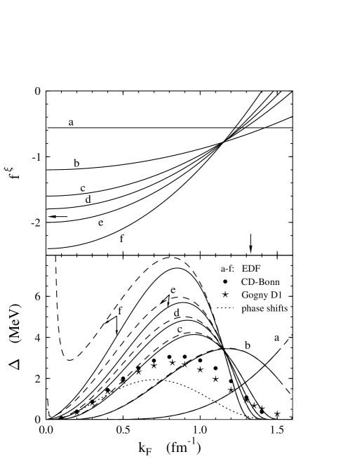
Figure 1: Dimensionless pairing strength (upper panel) and pairing gap (lower panel) in infinite nuclear matter as functions of the Fermi momentum. In the upper panel, the horizontal arrow shows the critical value of $f^{\xi}_{\rm ex}$ ($f^{\xi}_{\rm cr}=-1.912$) at which an $l=0$ spin singlet nucleon–nucleon bound state appears at zero energy while the vertical one marks the Fermi momentum at saturation point for the functional DF3 without pairing, $k_{0\rm F}=1.328$ fm^-1. In the lower panel, full (dashed) curves (a)–(f) are obtained by solving eqs. (4.6) and (4.9) (by using the weak pairing approximation, eq. (4.8)) with contact pairing force (4.2), and an energy cutoff $\epsilon_{\rm c}=40$ MeV, and correspond, respectively, to the parameter sets (a)–(f) of eq. (4.5). The solid circles and stars are the solutions of the nonlocal gap equation with the CD-Bonn potential [53] and with the finite-range Gogny D1 force [54], respectively. The dotted line shows the values of the pairing gap calculated using eq. (4.22) with the free NN scattering phase shifts (see text).

One should notice that $\epsilon_{\rm F}$ entering the integrand of the gap equation (4.6) can be expressed directly through density by $\epsilon_{\rm F}=\hbar^{2}k_{\rm F}^{2}/2m$ with $k_{\rm F}=(3\pi^{2}\rho/2)^{1/3}\equiv k_{0\rm F}x^{1/3}$ only if the pairing is weak indeed so that the dependence of the Fermi energy (and the chemical potential $\mu$) on $\Delta$ can be disregarded. Otherwise one should introduce the particle number condition

$$x=\frac{2}{\rho_{0}}\int\nolimits_{k\leq k_{\rm c}}\,\frac{\d\vec{k}}{(2\pi)^{3}}n_{k}(x)\,,$$ (4.9)

where

$$n_{k}(x)=\frac{1}{2}\left(1-\frac{\epsilon_{k}-\epsilon_{\rm F}(x)}{\sqrt{(\epsilon_{k}-\epsilon_{\rm F}(x))^{2}+\Delta^{2}(x)}}\right)\,,$$ (4.10)

and solve the system of the two equations (4.6) and (4.9) with respect to $\Delta$ and $\epsilon_{\rm F}$. The results shown in Fig. 1 by full lines correspond to such a direct solution while those shown by dashed lines to the weak pairing approximation, eq. (4.8).

As seen in Fig. 1, the approximation (4.8) works well in the entire range of $k_{\rm F}$ for the set (a), but for the other sets this is true only at $k_{\rm F}$ greater than $\approx$1.2 fm^-1 and also, for the sets (b), (c) and (d), at $k_{\rm F}$ less than 0.42, 0.14 and 0.042 fm^-1, respectively (in these regions the ratio $\Delta/\epsilon_{\rm F}$ does not exceed 0.1). For the sets (e) and (f), at lower densities, eq. (4.8) can not be used any more to estimate the gap even by order of magnitude since, as seen from the behavior of the corresponding dashed lines, it becomes divergent.

All parameter sets (4.5) except (a) reproduce the neutron separation energies and the isotope shifts of charge radii of lead isotopes reasonably well (see next section). For the sake of comparison also shown in Fig. 1 are the values of the ${}^{1}S_{0}$ pairing gap in nuclear matter obtained for the CD-Bonn potential without medium effects (using free single-particle spectrum $\epsilon_{k}=k^{2}/2m$) [53] and for the Gogny D1 force in the HFB framework [54]. The agreement between the two latter calculations is relatively good while both deviate noticeably from our predictions. The curve for contact density-independent pairing force, set (a), stands by itself with a positive derivative $\d\Delta(x)/\d x$ everywhere; no acceptable description of $\langle r^{2}_{\rm ch}\rangle$ could be obtained in this case (see Fig. 5). Interestingly, for the sets (b)–(e) which reproduce satisfactorily both the neutron separation energies $S_{\rm n}$ and mean squared charge radii $\langle r^{2}_{\rm ch}\rangle$ there exists a pivoting point at $k_{\rm F}\approx 1.15$ fm^-1 (at $\approx$0.65 of the equilibrium density) with the same value of $\Delta_{\rm piv}\approx 3.3$ MeV ($f^{\xi}_{\rm piv}\approx-0.78$).

One can see in Fig. 1 that for parameter sets with bigger absolute values of $f^{\xi}$ and $h^{\xi}$ the region where $\Delta(x)$ varies strongly moves towards lower densities, the slope becomes steeper and around $x\approx 1$ the pairing gap tends to be very small indeed. One may think that in finite nuclei the effect of the strong dependence of $\Delta$ on $x$, especially at small densities, would not influence the nuclear properties noticeably. But even if $\Delta$ would be concentrated only in the surface region and outside of the nucleus, the anomalous density, due to quantum effects, would not vanish inside the nucleus where $x\approx 1$. In this case the effect of density dependence should persist in the nuclear volume and should be more pronounced at larger values of $h^{\xi}$. This point was confirmed by our calculations (cf. Ref. [24] and below).

Consider in more detail the behavior of $\Delta$ at very low densities when $k_{\rm F}\rightarrow 0$ assuming the weak pairing regime, i.e. $f^{\xi}_{\rm ex}>f^{\xi}_{\rm cr}$ where $f^{\xi}_{\rm cr}$ is a critical strength constant given by

$$f^{\xi}_{\rm cr}=-2\frac{k_{0\rm F}}{k_{0\rm c}}\,,$$ (4.11)

with $k_{0\rm c}=\sqrt{2m\epsilon_{\rm c}}/\hbar$. This constant is determined by the condition

$$1+\frac{f^{\xi}_{\rm cr}}{4\sqrt{\epsilon_{0\rm F}}}\int_{0}^{\epsilon_{\rm c}}\frac{\d\epsilon}{\sqrt{\epsilon}}=0\,,$$ (4.12)

obtained from the gap equation (4.6) at $\Delta=\epsilon_{\rm F}=0$. For the chosen energy cutoff and parametrization (3.7) of our density functional we have $f^{\xi}_{\rm cr}=-1.912$. To leading order, on the other hand, at $k_{\rm F}\rightarrow 0$ from eq. (4.8) we obtain

$$\Delta=c\epsilon_{\rm F}\exp{\left(\frac{\pi}{2k_{\rm F}a}\right)}\,,\quad a<0\,,$$ (4.13)

where $c=8{\rm e}^{-2}\approx 1.083$ and where we have introduced the quantity

$$a=\frac{\pi}{2k_{0\rm F}}\left(\frac{\sqrt{2m\epsilon_{\rm c}}}{\hbar k_{0\rm F}}+\frac{2}{f^{\xi}_{\rm ex}}\right)^{-1}\equiv\frac{\pi}{4k_{0\rm F}}\left(\frac{1}{f^{\xi}_{\rm ex}}-\frac{1}{f^{\xi}_{\rm cr}}\right)^{-1}\,.$$ (4.14)

It can be shown that this quantity is nothing but the singlet nucleon–nucleon scattering length. To be more specific, consider first the two-neutron problem in the vicinity of the critical point, $f^{\xi}_{\rm ex}\approx f^{\xi}_{\rm cr}$, when the attraction is strong enough to produce a bound pair state (the scattering problem at any $f^{\xi}$ will be considered below). The bound-state wave function for the relative motion of two neutrons in case of contact interaction $C_{0}f^{\xi}_{\rm ex}\delta(\vec{r})$ is determined by (cf. Ref. [55]):

$$\psi(\vec{r})=-C_{0}f^{\xi}_{\rm ex}G_{0}(\vec{r},\epsilon_{\rm b})\psi(0)\,,$$ (4.15)

where $G_{0}$ is the free Green’s function in the truncated space,

$$G_{0}(\vec{r},\epsilon_{\rm b})=\int\nolimits_{\epsilon_{k}^{\rm nn}\leq\epsilon_{\rm c}^{\rm nn}}\,\frac{\d\vec{k}}{(2\pi)^{3}}\frac{{\mathrm{e}}^{{\mathrm{i}}\vec{k}\vec{r}}}{\epsilon_{k}^{\rm nn}-\epsilon_{\rm b}}\,,$$ (4.16)

with $\epsilon_{\rm b}$ the binding energy and $\epsilon_{k}^{\rm nn}=\hbar^{2}k^{2}/m$ (the reduced mass is $m/2$). In the rest system of a nucleus, the center-of-mass energy $\epsilon^{\rm nn}$ in the scattering problem would correspond to the energy $\epsilon^{\rm nn}/2$ of each of the two nucleons in the $s$-wave pairing problem. This implies that the cutoff in the $k$-space in eq. (4.16), $k_{\rm c}^{\rm nn}=\sqrt{m\epsilon_{\rm c}^{\rm nn}}/\hbar$, should be the same as in the gap equation. Thus, in the energy space, one has $\epsilon_{\rm c}^{\rm nn}=2\epsilon_{\rm c}$ and from (4.15) at $\vec{r}=0$ one obtains the equation to determine $\epsilon_{\rm b}$:

$$1=-\frac{1}{4\sqrt{\epsilon_{0\rm F}}}f^{\xi}_{\rm ex}\int_{0}^{\epsilon_{\rm c}}\d\epsilon\frac{\sqrt{\epsilon}}{\epsilon-\epsilon_{\rm b}/2}\,,$$ (4.17)

which reduces to

$$\frac{f^{\xi}_{\rm ex}}{f^{\xi{\rm nn}}_{\rm cr}}=\left(1-\sqrt{\frac{-\epsilon_{\rm b}}{2\epsilon_{\rm c}}}\arctan{\sqrt{\frac{2\epsilon_{\rm c}}{-\epsilon_{\rm b}}}}\right)^{-1}\,,$$ (4.18)

where $f^{\xi{\rm nn}}_{\rm cr}$ is a critical value of $f^{\xi}_{\rm ex}$ at which eq. (4.15) has a bound state solution $\epsilon_{\rm b}=0$. Comparing eq. (4.17) at $\epsilon_{\rm b}=0$ with eq. (4.12) one finds that $f^{\xi{\rm nn}}_{\rm cr}$ coincides with the value defined above by eq. (4.11). Now, in the vicinity of $f^{\xi}_{\rm cr}$ we can set $\arctan{\sqrt{2\epsilon_{\rm c}/|\epsilon_{\rm b}|}}\approx\pi/2$ and use $\epsilon_{\rm b}=-\hbar^{2}/ma^{2}_{\rm nn}$ in eq. (4.18). Then it is easy to see that the solution for the scattering length $a_{\rm nn}$ is exactly the same as given by (4.14). The expression (4.13) for $\Delta$ agrees with the results of Ref. [40] based on a general analysis of the gap equation at low densities when $k_{\rm F}|a|\ll 1$. But we should stress that (4.13) is valid only in the weak-coupling regime corresponding to negative $a$. In the opposite case the gap in the dilute limit has to be found in a different way.

At $f^{\xi}_{\rm ex}>f^{\xi}_{\rm cr}$ the scattering length is negative, and from eq. (4.13) it follows that at low densities the pairing gap is exponentially small and eventually $\Delta(k_{\rm F}\rightarrow 0)=0$. Such a weak pairing regime with Cooper pairs forming in a spin singlet $l=0$ state exists up to the critical point at which the attraction becomes strong enough to change the sign of the scattering length. Then the strong pairing regime sets in, eqs. (4.8) and (4.13) are not valid any more, and $\Delta$ should be determined directly from the combined solution of the gap equation (4.6) and the particle number condition (4.9). In the dilute systems, $\epsilon_{\rm F}$ plays the role of the chemical potential $\mu$. The latter is defined by $\mu=\epsilon_{\rm F}(k_{\rm F})+U(k_{\rm F})$ with $U(k_{\rm F})$ the HF mean field at the Fermi surface which is negligible for the fermion gas. At the critical point $\mu$ becomes negative and a bound state of a single pair of nucleons with the binding energy $\epsilon_{\rm b}=2\mu$ becomes possible [56, 57]. This can be easily seen from the gap equation (4.6) written in the form

$$\left(\frac{k^{2}}{m}-2\mu\right)\phi_{k}=-{\rm sgn}(\epsilon_{k}-\mu)\sqrt{1-\phi_{k}^{2}}\int\nolimits_{k\,^{\prime}\leq k_{\rm c}}\,\frac{\d\vec{k}\,^{\prime}}{(2\pi)^{3}}{\mathcal{F}}^{\xi}\phi_{k\,^{\prime}}\,,$$ (4.19)

where we have introduced the functions $\phi_{k}=\Delta/\sqrt{(\epsilon_{k}-\mu)^{2}+\Delta^{2}}$ and replaced $\epsilon_{\rm F}$ by $\mu$. In the strong coupling regime, $\mu<0$, and in the dilute limit, $|\phi_{k}|\ll 1$, this equation reduces to the Schrödinger equation for a single bound pair where $2\mu$ plays the role of the eigenvalue. It is equivalent to the coordinate-space equation (4.15). Thus $2\mu=\epsilon_{\rm b}$ where the binding energy $\epsilon_{\rm b}$ is determined from (4.18). The pairing gap $\Delta$ at low densities in this regime can be found from the particle number condition (4.9) which in the leading order now reads

$$x=\frac{3\Delta^{2}}{8\epsilon_{0\rm F}^{3/2}}\int_{0}^{\epsilon_{\rm c}}\frac{\sqrt{\epsilon}\d\epsilon}{(\epsilon+|\mu|)^{2}}\,.$$ (4.20)

In the vicinity of the critical point from this equation we find

$$\Delta^{2}=\frac{16}{3\pi}x\epsilon_{0\rm F}^{2}\frac{1}{k_{0\rm F}a}\,,$$

which gives

$$\Delta=\frac{\hbar^{2}}{m}\left(\frac{2\pi\rho}{a}\right)^{1/2}\,,\quad a>0\,.$$ (4.21)

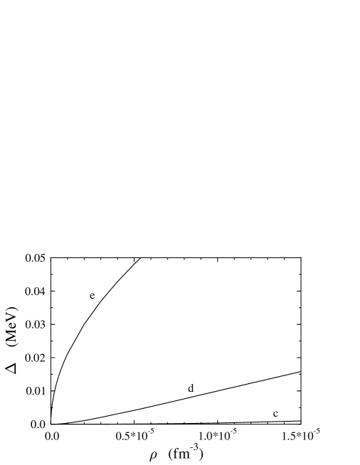
Figure 2: Pairing gap $\Delta$ as a function of $\rho$ at very low densities. Curves (c)–(e) correspond to the parameter sets (c)–(e) of eq. (4.5), respectively.

From this consideration it follows that, in the dilute case, the energy needed to break a condensed pair goes smoothly from $2\Delta$ to $2\mu=\epsilon_{\rm b}$ as a function of the coupling strength when the regime changes from weak to strong pairing. But as seen from (4.13) and (4.21), the behavior of $\Delta$ at low densities is such that the derivative $\d\Delta/\d\rho$ at $\rho\rightarrow 0$ as a function of $f^{\xi}_{\rm ex}$ exhibits a discontinuity from 0 to $\infty$. This is illustrated in Fig. 2 where we have plotted the gap $\Delta(\rho)$ at very low densities for the sets (c)–(e) of eq. (4.5) embracing both regimes. We note also that the analytical expressions (4.13) and (4.21) give a purely imaginary gap at the critical point when the scattering length changes sign ($k_{\rm F}a\rightarrow\sqrt{2m\mu}/\hbar\rightarrow{\mathrm{i}}$ if $\mu$ becomes negative). In this connection it is instructive to write the weak coupling expression (4.8) for $\Delta$ in the following form [58]:

$$\Delta(k_{\rm F})=c\epsilon_{\rm F}\exp\left[-\frac{\pi}{2}\cot\delta(k_{\rm F})\right]\,,$$ (4.22)

where $c=8{\rm e}^{-2}$ and where we have introduced the Fermi level phase shift $\delta(k_{\rm F})$ defined by

$$k_{\rm F}\cot\delta(k_{\rm F})=-\frac{4k_{0\rm F}}{\pi}\left(\frac{1}{f^{\xi}(k_{\rm F})}+\frac{k_{\rm c}(k_{\rm F})}{2k_{0{\rm F}}}\right)-\frac{k_{\rm F}}{\pi}\ln\left(\frac{k_{\rm c}(k_{\rm F})-k_{\rm F}}{k_{\rm c}(k_{\rm F})+k_{\rm F}}\right)\,,$$ (4.23)

with $k_{\rm c}(k_{\rm F})=\sqrt{k_{0\rm c}^{2}+k_{\rm F}^{2}}$. Eq. (4.23) corresponds to an exact solution of the nn scattering problem at the relative momentum $k=k_{\rm F}$ with the states truncated by a momentum cutoff $k_{\rm c}=k_{\rm c}(k_{\rm F})$ for contact interaction $C_{0}f^{\xi}(k_{\rm F})\delta({\vec{r}})$ (see, e.g., Ref. [59]). In the dilute limit, from eq. (4.22) one notices again that the pairing gap becomes pure imaginary at the critical point since $\cot\delta\rightarrow{\mathrm{i}}$ when $|a_{\rm nn}|\rightarrow\infty$. At very low densities, with the parametrization (4.3) of the pairing force and with the chosen density-dependent cutoff, eq. (4.23) reduces to

$$k_{\rm F}\cot\delta(k_{\rm F})\approx-\frac{1}{a_{\rm nn}}+\frac{1}{2}r_{\rm nn}k_{\rm F}^{2}-\frac{2k_{\rm F}}{\pi}\left[\frac{k_{\rm F}}{2k_{0\rm c}}-\frac{2h^{\xi}}{(f^{\xi}_{\rm ex})^{2}}\left(\frac{k_{\rm F}}{k_{0\rm F}}\right)^{3q-1}\right]\,,$$ (4.24)

where $a_{\rm nn}$ is the scattering length defined by eq. (4.14) and $r_{\rm nn}$ is the effective range, $r_{\rm nn}=4/\pi k_{0\rm c}$. The first two terms in this equation would describe low-energy behavior of the nn $s$-wave phase shift through an expansion of $k\cot\delta$ in powers of the relative momentum $k=k_{\rm F}$ if the interaction were density-independent – in our case, if the coupling strength and momentum cutoff were fixed by $f^{\xi}=f^{\xi}_{\rm ex}$ and $k_{\rm c}=k_{0\rm c}$, respectively. It follows that with a density-dependent effective force, such an expansion contains additional terms which for the parametrization used here are of the same order as the effective range term. This simply demonstrates that, for reproducing the pairing gap, the effective interaction even at very low densities need not necessarily coincide with the bare NN interaction.

When the Fermi momentum $k_{\rm F}$ approaches from below the upper critical point at which the pairing gap closes, $k_{\rm F}^{\rm cr}=k_{0{\rm F}}(-f^{\xi}_{\rm ex}/h^{\xi})^{1/3q}$ defined by $f^{\xi}(k_{\rm F})=0$, we get from eq. (4.22)

$$\Delta(k_{\rm F})\approx c\epsilon_{\rm F}\exp\left[-\frac{2k_{0{\rm F}}}{3qf^{\xi}_{\rm ex}(k_{\rm F}-k_{\rm F}^{\rm cr})}\right]\,.$$ (4.25)

Thus, at higher densities, the pairing gap becomes exponentially small when $k_{\rm F}$ approaches $k_{\rm F}^{\rm cr}$, in agreement with general analysis of the gap solutions [40]. In weak coupling, as we have already shown, $\Delta(k_{\rm F})$ is also exponentially small at low densities, in the vicinity of $k_{\rm F}=0$. It is noteworthy that near both critical points the pairing potential $\Delta$ can be found from the behavior of the phase shift by using eq. (4.22) with a smooth density-dependent prefactor $c(k_{\rm F})$ (the details will be given elsewhere [61]). In the present paper, as an illustration, we show in Fig. 1 by the dotted line the values of $\Delta(k_{\rm F})$ obtained from eq. (4.22), with a prefactor $c=8{\rm e}^{-2}$, by using “experimental” nn phase shifts, without electromagnetic effects. It is seen that $\Delta$ obtained this way at low densities closely follows the solution of the gap equation with the CD-Bonn potential [53]. The nn phase shift passes zero at the relative momentum $k\approx 1.71$ fm^-1, and the gap should vanish at the corresponding Fermi momentum. Unfortunately, the solutions for $\Delta$ are given in Ref. [53] only in the region up to $k_{\rm F}=1.4$ fm^-1 which is rather far from the upper critical point.

For symmetric nuclear matter, with the functional DF3 used in the present paper, the energy per particle is

$$\frac{E}{A}(x)=\frac{2}{\rho_{0}x}\int\nolimits_{k\leq k_{\rm c}}\frac{\d\vec{k}}{(2\pi)^{3}}\frac{\hbar^{2}k^{2}}{2m}n_{k}(x)+\frac{1}{3}\epsilon_{0\rm F}a_{+}^{\rm v}f_{+}^{\rm v}(x)x+\frac{3\Delta^{2}(x)}{2f^{\xi}(x)x\epsilon_{0\rm F}}\,,$$ (4.26)

where $f_{+}^{\rm v}(x)=(1-h^{\rm v}_{1+}x)/(1+h^{\rm v}_{2+}x)$ with the parameters given by (3.7); here the “particle–hole” term $\propto f_{+}^{\rm v}$ vanishes in the dilute limit linearly in density. The chemical potential is

$$\mu(x)=\epsilon_{\rm F}(x)+\frac{1}{3}\epsilon_{0\rm F}a_{+}^{\rm v}[f^{{\rm v}\prime}_{+}(x)x^{2}+2f^{\rm v}_{+}(x)x]+\frac{3f^{\xi\prime}(x)}{2f^{\xi 2}(x)}\frac{\Delta^{2}(x)}{\epsilon_{0\rm F}}\,,$$ (4.27)

where the prime denotes the derivative with respect to the dimensionless density $x$. The Fermi energy $\epsilon_{\rm F}(x)$ and the pairing gap $\Delta(x)$ entering these equations are determined from (4.6) and (4.9). The last two terms in (4.27), even in strong pairing regime, vanish in the dilute limit at least as $x^{q}$ if $0<q<1$ or linearly in $x$ if $q\geq 1$ (in our case, the exponent in the density-dependent pairing force is $q=\frac{2}{3}$). Thus, we see again that, in strong coupling, in the leading order $\mu=\epsilon_{\rm F}=\epsilon_{\rm b}/2<0$.

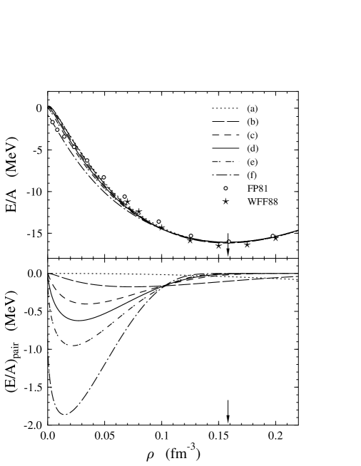
Figure 3: Energy per nucleon $E/A$ (top) and pairing contribution to $E/A$ (bottom) in symmetric nuclear matter. Curves (a)–(e) are calculated using eq. (4.26) and correspond to the strength parameters (a)–(e) of eq. (4.5), respectively. Open circles and stars are the calculations of Ref. [62] and Ref. [63], respectively, for the UV14 plus TNI model. The vertical arrows mark the saturation density for the functional DF3 without pairing, $2\rho_{0}=0.1582$ fm^-3.

The calculated energy per nucleon as a function of the isoscalar density $\rho$ is shown in the upper panel in Fig. 3 together with the results of the nuclear matter calculations [62, 63] for the UV14 plus TNI model. It is seen that DF3 gives qualitatively reasonable description of the nuclear matter EOS and that pairing could contribute noticeably to the binding energy especially at lower densities. In the lower panel in Fig. 3 we have plotted the pairing energy per nucleon, $(E/A)_{\rm pair}$, obtained by subtracting from eq. (4.26) the corresponding value of $E/A$ at $\Delta=0$. This pairing energy is a sum of the positive contribution coming from the kinetic energy, i.e. from the first term in (4.26), and the negative anomalous energy – the last term in (4.26) (an expression for $(E/A)_{\rm pair}$ in the case of weak pairing is derived in Appendix B). The pairing contribution is small for the density-independent force with $f^{\xi}=0.56$, set (a) of eq. (4.5), and increases, as expected, for the sets (b)–(f) with a shift to lower densities as $f^{\xi}_{\rm ex}$ becomes gradually more attractive. For the sets (e) and (f) the attraction is strong, $f^{\xi}_{\rm ex}<f^{\xi}_{\rm cr}$. In these cases a nonvanishing binding energy in the dilute limit is solely due to Bose-Einstein condensation of the bound pairs, the spin-zero bosons, when all the three quantities, $\mu$, $E/A$ and $(E/A)_{\rm pair}$, reach the same value $\epsilon_{\rm b}/2$ ($\epsilon_{b}=-0.0646$ and $-1.616$ MeV for the set (e) and (f), respectively). This is illustrated in Fig. 4 where we have plotted $E/A$ and $(E/A)_{\rm pair}$ as functions of $\rho$ at very low densities. Analytically, for the kinetic energy term in (4.26) in the leading order we find

$$\frac{E_{\rm kin}}{A}=\frac{3\Delta^{2}}{8x\epsilon_{0\rm F}^{3/2}}\int_{0}^{\epsilon_{\rm c}}\frac{\epsilon\sqrt{\epsilon}\d\epsilon}{(\epsilon+|\mu|)^{2}}\approx\frac{3\Delta^{2}}{2x\epsilon_{0\rm F}}\left(-\frac{1}{f^{\xi}_{\rm cr}}-\frac{3\pi}{8}\frac{1}{k_{0\rm F}a}\right)\,,$$ (4.28)

where we have used the definition (4.11) and the relation $|\mu|=\hbar^{2}/2ma^{2}$. Combining this with the last term in (4.26), one gets

$$\frac{E}{A}=-\frac{3\pi\Delta^{2}}{16x\epsilon_{0\rm F}}\frac{1}{k_{0\rm F}a}\,.$$ (4.29)

By using eq. (4.21), this expression reduces exactly to $-\hbar^{2}/2ma^{2}=\epsilon_{\rm b}/2$. It follows that the model just described is in fact parameter-free: in the strong coupling regime near the critical point, the ground state properties of nuclear matter in the dilute limit are completely determined by the scattering length.

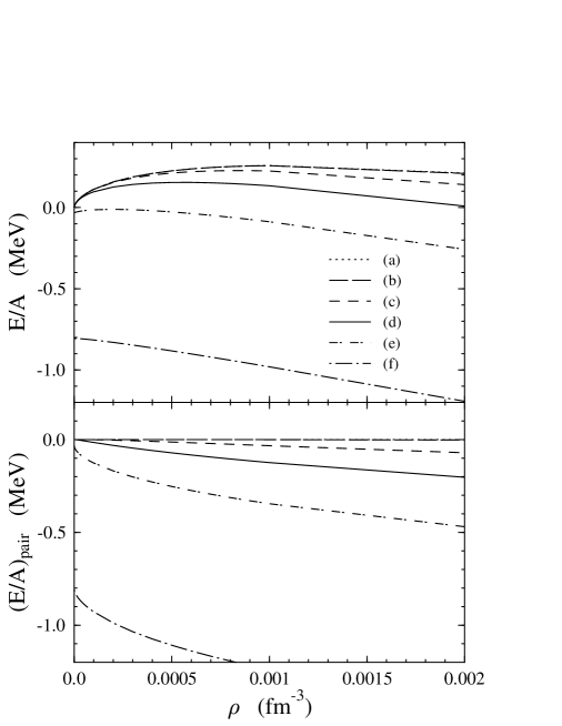
Figure 4: Energy per nucleon $E/A$ (top) and pairing contribution to $E/A$ (bottom) for symmetric nuclear matter at low densities. The notations are the same as in Fig. 3.

We have considered subsaturated nuclear matter with ${}^{1}S_{0}$ pairing within our local EDF framework and demonstrated some results, including extrapolation to the low density limit, with a few possible parameter sets of the pairing force deduced from experimental data for lead isotopes. At low densities, in the $T=0$ case of symmetric $N=Z$ matter, the ${}^{3}S_{1}-^{3}D_{1}$ pairing correlations leading to a Bose deuteron gas formation might be more important since the n–p force is more attractive than that in the p–p or n–n pairing channels (see Ref. [64] and references therein). Thus, our approach, with ${}^{1}S_{0}$ pairing only, would be more relevant for an asymmetric $N\neq Z$ case and for pure neutron systems. From this point of view the best choice of the effective contact pairing force for the EDF calculations seems to be the set (d) of eq. (4.5) since it gives the singlet scattering length $a_{\rm nn}\approx-17.2$ fm which corresponds to a virtual state at $\approx 140$ keV known experimentally. As seen in Fig. 1, with this choice the behavior of $\Delta$ at low densities agrees well with the calculations based on realistic NN forces. At higher densities, however, our predictions for $\Delta$ with the set (d) go much higher reaching a maximum of $\approx 4.84$ MeV at $k_{\rm F}\approx 0.92$ fm^-1 while the calculations of Ref. [53] give a maximum of about 3 MeV at $k_{\rm F}\approx 0.82$ fm^-1. With a bare NN interaction, assuming charge independence and $m_{\rm n}=m_{\rm p}$ in the free single-particle energies, the pairing gap would be, at given $k_{\rm F}$, exactly the same both in symmetric nuclear matter and in neutron matter. As shown in Refs. [65, 66], if one includes medium effects in the effective pairing interaction, most importantly the polarization RPA diagrams in the cross channel, the pairing gap in neutron matter would be substantially reduced to values of the order of 1 MeV at the most. Whether such a mechanism works in the same direction for symmetric nuclear matter is still an open question. If the gap were smaller than that obtained with the Gogny D1 force, which is also shown in Fig. 1, it would be difficult to explain the observed nuclear pairing properties. The effective contact density-dependent force (4.3) with our preferable parameter set (d) of eq. (4.5) yields larger pairing energy in nuclear matter than the Gogny force, but in finite nuclei this is compensated by the repulsive gradient term. The phenomenological pairing force used here contains dependence on the isoscalar density only since we have analyzed the existing data on separation energies and charge radii for finite nuclei with a relatively small asymmetry characterized by $(N-Z)/A\leq 0.25$. An extrapolation to neutron matter with such a simple force would give a larger pairing gap than for nuclear matter. This suggests that some additional dependence on the isovector density $\rho_{\rm n}-\rho_{\rm p}$ might be present in the effective pairing force. This possibility is planned to be tested in our future work, with a more careful analysis of experimental data though the relevant data base is not rich enough.

Now consider how the density changes when the pairing gap appears in nuclear matter. To leading order, one finds the following expression for the energy per nucleon near the saturation point:

$$\frac{E}{A}=\frac{E_{0}}{A}+\frac{K_{0}}{18}\frac{(x-x_{0})^{2}}{x_{0}^{2}}+\beta(x)I^{2}-\frac{3}{8}\frac{\Delta^{2}(x)}{\epsilon_{\rm F}(x)}\,$$ (4.30)

where $K_{0}$ is the compression modulus at saturation density, $\beta(x)I^{2}$ is the asymmetry energy, with $I=(\rho_{\rm n}-\rho_{\rm p})/2\rho_{0}x\equiv(N-Z)/A$. This expression is valid at $|x-x_{0}|\ll 1,\,|I|\ll 1$ and $\Delta\ll\epsilon_{\rm F}$. Higher order effects connected with $I$-dependence of $K,\beta,\Delta$ and $\epsilon_{\rm F}$ are neglected. The derivation of the last term in (4.30) is discussed in detail in Appendix B. Due to this pairing term, the position of the equilibrium point may be shifted to lower or higher densities depending on the behavior of $\Delta(x)$ near $x=1$. If $\Delta$ does not depend on $x$ in the vicinity of $x=1$ then the equilibrium density decreases due to presence of $\epsilon_{\rm F}(x)\propto x^{2/3}$ in the denominator of the pairing term (the system gains more binding energy). This means an expansion of the system. The effect is enhanced if $\Delta$ becomes larger during such an expansion, i.e. when the derivative $\d\Delta(x)/\d x$ at $x=1$ is negative. This point may be illustrated by the following simple consideration. At equilibrium the pressure $P=0$ which means

$$\frac{\partial}{\partial x}(E/A)=0\,.$$ (4.31)

For saturated symmetric nuclear matter without pairing the dimensionless density is, by definition, $x_{0}=1$. When $I\neq 0$ and $\Delta\neq 0$, from eq. (4.30) with condition (4.31) the new equilibrium density can be found (in units of $2\rho_{0}$), which is the solution of the equation

$$x-x_{0}=\frac{9x_{0}^{2}}{K_{0}}\left[\frac{\Delta(x)}{4\epsilon_{\rm F}(x)}\left(3\frac{\d\Delta(x)}{\d x}-\frac{\Delta(x)}{x}\right)-\frac{\d\beta(x)}{\d x}I^{2}\right]\,.$$ (4.32)

From this equation one can see that the density should be sensitive indeed to the derivatives of $\Delta$, and a negative slope in $\Delta$ should cause a decrease of the density. The obtained relations can be used to estimate the influence of pairing on the charge radii for heavy nuclei as was done in Ref. [22]. It was shown that pairing interaction with strong $\rho$-dependence at $x\approx 1$ might significantly change the equilibrium density. For the parametrization used here the size of this effect is controlled by the parameter $h^{\xi}$. The shift of the saturation point is relatively small: $|\delta\rho|/2\rho_{0}\leq 0.8$ % for all the six sets of eq. (4.5) ($\delta\rho/2\rho_{0}\approx+0.4$ % and $\approx-0.4$ % for the set (a) and (d), respectively). In finite nuclei, the surface term $\propto f^{\xi}_{\nabla}$ is equally important to produce a kink in the radius evolution along isotope chain at magic neutron number and, especially, to explain the observed odd-even staggering in $\langle r^{2}_{\rm ch}\rangle$ [24]. Although, as seen in Fig. 1, the calculations with bare NN interaction or with Gogny force give a negative sign for $\d\Delta(x)/\d x$ near $x\approx 1$ ($k_{\rm F}\approx 1.33$ fm^-1), but the slope might be not steep enough. This is the probable reason why the HFB calculations with the Gogny force, which give a good description of the global pairing properties of nuclei, could not reproduce the kink in lead isotopes [67]. The density dependence of the pairing force leads to the direct coupling between the neutron anomalous density and the proton mean field as given by (4.4). The suppression of $|\nu_{\rm n}|^{2}$ in the odd neutron subsystem because of the blocking effect influences the potential $U^{\rm p}_{\rm pair}$ of the proton subsystem through the volume, $\propto h^{\xi}$, and surface, $\propto f^{\xi}_{\nabla}$, couplings, and this moves the behavior of the proton radii towards the desired regime [24].

5 Numerical results for some isotope chains

The calculations for finite spherical nuclei are performed using the coordinate-space technique which is described in detail in Appendix C. In the construction of the Gor’kov Green’s functions, the four linear-independent solutions $(u_{i},v_{i})\,,i=1$–4, were found by the Numerov method with a radial step of 0.1 fm and physical boundary conditions imposed for each $lj$ channel at the origin and at $r=25$ fm. The contour in the complex energy plane with Im$\epsilon=\pm 8$ MeV along the horizontal sections and with energy cutoff $\epsilon_{\rm c}=40$ MeV measured from the Fermi level was used (see Figs. 21, 22 in Appendix C). The integration along the contour was performed by the Simpson method with automatic step selection. The convergence of the iteration procedure is controlled by a few criteria: for two successive steps $i$ and $i+1$, the conditions $|\rho_{i+1}(r)-\rho_{i}(r)|<10^{-6}$ fm^-3 and $|\Delta_{i+1}(r)-\Delta_{i}(r)|<50$ keV should be achieved for all $r$, the chemical potential $\mu$ should finally satisfy the condition $|N(\mu)-N|<0.01$ and the contribution $N_{lj}$ to the total particle number $N(\mu)$ from the states with higher angular momenta $lj$ should not exceed 0.01. Such criteria guarantee an accuracy not worse than 0.1% for all the calculated quantities of our interest. The mean square charge radii were computed from ground state charge densities obtained by folding the point nucleon distributions with nucleon charge form factors, including the relativistic electromagnetic spin–orbit correction, in the same way as in Ref. [68].

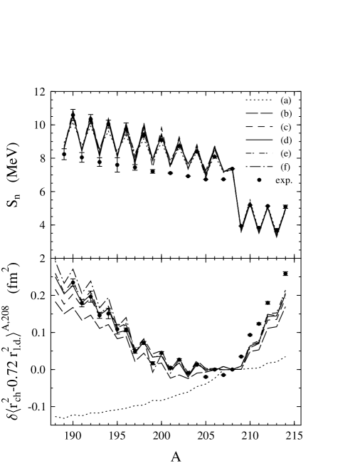
Figure 5: Upper panel: neutron separation energies $S_{\rm n}$ for lead isotopes. Lower panel: differences of mean squared charge radii $\delta\langle r^{2}_{\rm ch}\rangle$ with respect to ²⁰⁸Pb as reference nucleus; 72% of the corresponding liquid drop values (using $r_{0}=1.1$ fm) are subtracted to enhance the visibility of the small differences. The calculations are performed with the functional DF3 and the coordinate-space technique. Curves (a)–(f) connect the points obtained with parameter sets (a)–(f) of the pairing force (4.5), respectively. Experimental data for $S_{\rm n}$, including those derived from systematic trends, are from [69, 70]; data for $\delta\langle r^{2}_{\rm ch}\rangle$ are from [71, 72, 73].

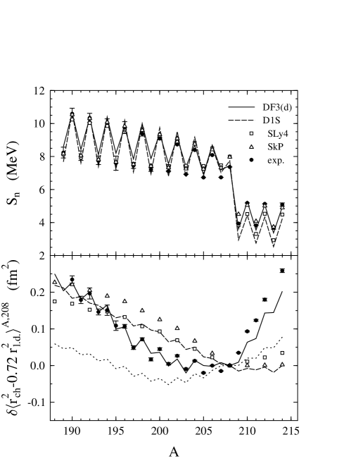
Figure 6: The same as in Fig. 5 but only for the set (d) of the pairing force in comparison with the HFB calculations with Skyrme forces SkP [74] and SLy4 [8, 75], and the Gogny D1S [76] force. Also shown in the lower panel by the dotted line are the $\delta\langle r^{2}_{\rm ch}\rangle$ values obtained without gradient term in the pairing force ($f^{\xi}_{\rm ex}=-1.79,\;h^{\xi}=1.66,\;f^{\xi}_{\nabla}=0$).

Let us discuss first the results obtained for the lead chain. As shown in the upper panel of Fig. 5, the experimental neutron separation energies are reproduced equally well for all the chosen parameter sets of the pairing force. The curves (a)–(f) correspond to the sets marked with the same letters in eq. (4.5). The curve (a) is obtained for the “constant” pairing force, without density dependence. The other sets (b)–(f) differ from that by non-zero values of $h^{\xi}$ and $f^{\xi}_{\nabla}$ parameters. As already mentioned in Section 4, for each $f^{\xi}_{\rm ex}$ value it is possible to find such values of $h^{\xi}$ and $f^{\xi}_{\nabla}$ that the pairing energy for a given nucleus is practically the same. These parameters are kept fixed for all isotopes of the lead chain.

In the lower panel of Fig. 5 the calculated isotope shifts of mean squared charge radii, $\delta\langle r^{2}_{\rm ch}\rangle$, for the lead chain with respect to ²⁰⁸Pb as a reference nucleus are presented. These curves except (a) do not differ from each other significantly and all of them reproduce qualitatively the kink and the average size of odd-even staggering. The curve (a) corresponds to a simple pairing delta-force; in this case the behavior of $\delta\langle r^{2}_{\rm ch}\rangle$ is rather smooth and neither kink nor staggering are reproduced. The variant (a) of eq. (4.5) was included just to give an example that without any density dependence in the contact pairing effective interaction it is also possible to describe the neutron separation energies but not the evolution of charge radii. With the parametrization of eq. (4.3) used here for the pairing force, the size of the staggering and the kink in charge radii of Pb isotopes can be reproduced only if the “gradient” parameter $f^{\xi}_{\nabla}$ is $\approx 2$. Without gradient term the results for radii would be in between the curves (a) and (b) shown in the lower panel of Fig. 5 (an example is given in the lower panel of Fig. 6). On the whole, as seen in Fig. 5, the set (d) yields a somewhat better description than the other sets, particularly for the lighter Pb isotopes. For this reason, and due to the fact that the set (d) corresponds to the correct value of the singlet scattering length in the dilute limit (see previous Section), this set will be taken as our preferable choice, and the corresponding functional will be referred to as DF3(d) in the following.

In Fig. 6 we compare the DF3(d) predictions for Pb isotopes with the HFB results obtained for the Gogny D1S force [76] and for two state-of-the-art models based on Skyrme density-dependent forces SkP [74]and SLy4 [75]. The calculations with Gogny force for the odd isotopes are done in the blocking approximation, and thus we can show the results both for even and odd Pb isotopes. The Skyrme-HFB calculations were done, unfortunately, without blocking, and therefore we show the radii only for even isotopes; the $S_{n}$ values for odd isotopes were obtained by correcting the no-blocking HFB energy by adding an average pairing gap, this was considered to be a very good approximation. The details of the HFB+SkP and HFB+SLy4 calculations can be found in [77] (see also the references therein), and here we only briefly discuss how the pairing correlations have been implemented in these models. The HFB+SkP calculations have been done with the same SkP force in the ph and pp channels, and therefore in these calculations the pairing force has density dependence $x^{1/6}$. The energy cutoff has been chosen by including the quasi-particle states up to the energy equal to the depth of the effective single-particle potential [74]. This implies that the cutoff depends not only on the particle numbers $N$ and $Z$ but also on the quantum numbers $j$ and $l$; for $l$=0 it varies in the range of about 40–50 MeV. The HFB+SLy4 calculations have been done with the density-dependent zero-range pairing force in the pp channel, and the SLy4 force in the ph channel. The form of this pairing force is identical to the velocity-independent piece of the Skyrme interaction (see Ref. [78]) with parameters $V_{0}=t_{0}=-2488.913$ MeV fm³ and $V_{3}=19990$ MeV fm^3+1/6, and it also has the $x^{1/6}$ density dependence. The prescription for the energy cutoff has been identical as in the HFB+SkP calculations. We remark that such a prescription is much different from that which we use here; with such a recipe it is not easy to construct the corresponding effective contact pairing force with a fixed phase-space cutoff, hence no simple extrapolation to the pairing properties of uniform nuclear matter.

One can see in the upper panel of Fig. 6 that the HFB+D1S, HFB+SkP, SkLy4 and our DF3(d) calculations describe the neutron separation energies with more or less the same quality, some deviations are observed in the region above ²⁰⁷Pb. For the lighter Pb isotopes, the Gogny force slightly overestimates the odd-even effect in $S_{n}$ while with DF3(d) it is slightly underestimated.

In the lower panel of Fig. 6 it is seen that the Skyrme-HFB calculations with SkP and SLy4 forces give too small kink in radii. Calculations with the Gogny D1S force for $\delta\langle r^{2}_{\rm ch}\rangle$ could not reproduce the kink either. The latter model yields sizeable staggering in radii, but the effect is too small, at least by a factor of two smaller in amplitude than experimentally observed; moreover, its sign in isotopes below $A$=194 is reversed with respect to the observations. As for the Skyrme functionals, one suspects that they could not give the correct size of staggering as well. Such a conclusion may be supported by our DF3 calculations with parameters $f^{\xi}_{\rm ex}=-1.79,\;h^{\xi}=1.66,\;f^{\xi}_{\nabla}=0$, i.e. with the pairing force of (4.5) which contains only a $x^{2/3}$ dependence, without gradient of density. The external strength constant $f^{\xi}_{\rm ex}=-1.79$ is taken from our preferable set (d), and the parameter $h^{\xi}=1.66$ is found to get practically the same $S_{n}$ values as with the variant (d) itself. The results for the radii are shown in the lower panel of Fig. 6 by the dotted line. It is seen that the staggering appears but it is too small indeed. With a $x^{1/6}$ dependence, which is used with the SkP and SLy4 parametrization, the effect would be even smaller. Thus, to reproduce the scale of the odd-even effects in radii (and the scale of the kinks) within the local energy-density functional approach, the blocking mechanism should be enhanced by some peculiar density dependence of the effective pairing force, the linear dependence on $\rho^{\sigma}$ with $\sigma$=1, 1/3, 1/6… could not give the desirable size.

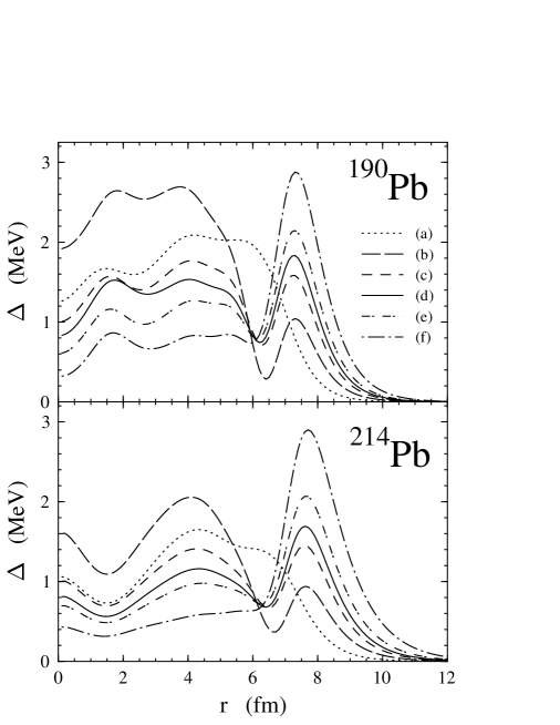
Figure 7: Pairing gap $\Delta$ for ¹⁹⁰Pb (top) and ²¹⁴Pb (bottom) as a function of the radial coordinate $r$. The curves are marked in the same way as in Fig. 5.

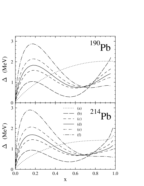
Figure 8: Pairing gap $\Delta$ for ¹⁹⁰Pb (top) and ²¹⁴Pb (bottom) as a function of the dimensionless isoscalar density $x$. The curves are marked in the same way as in Fig. 5.

This fact clearly demonstrates the importance of including odd-mass nuclei in the fitting procedure of force constants. Now, in general, a complete description of the ground state of an odd nucleus is quite difficult which reflects itself e.g. in the difficulty to reproduce experimental magnetic moments. These depend sensitively on the time-reversal-odd components of the polarization induced by the odd particle. However, the operator $r^{2}$ is time-reversal-even, and the small, not-well-known, odd components of the polarization enter the expectation value only quadratically. If, with given interaction, $\langle r^{2}\rangle$ is not well described by a HFB-type ground state, there is no hope to reproduce it with a more sophisticated state vector. As can be seen from Figs. 5 and 6, it is possible to reproduce the order of magnitude of the staggering of $\langle r^{2}\rangle$ with density-dependent pairing force (4.3) containing a gradient term.

Similar arguments apply to the nuclei off magic numbers. Looking only at even neutron isotopes, the slope of $\langle r^{2}\rangle$ as a function of $N$ changes at the magic numbers, producing a “kink”. With simple interactions in the pp-channel, this is not reproduced in HFB-type calculations. This relative increase of $\langle r^{2}\rangle$ off magic numbers is thought to be connected with “dynamical deformation” due to ground state fluctuations of the surface. These ground state fluctuations of the surface, being time-independent, actually can not be separated from a static diffuseness of the surface, and are present in an independent particle model too. In Section 6 below we will give some estimates of the contribution of RPA-type ground state correlations to this effect. It emerges that the main part of the effect should—and can—be obtained on the HFB level.

In Fig. 7 the $r$-dependence of $\Delta$ for two isotopes ¹⁹⁰Pb and ²¹⁴Pb (the ends of the measured chain) is shown. One can see that with increasing external attraction $\propto f^{\xi}_{\rm ex}$, $\Delta$ becomes smaller in the volume and gradually concentrates in the outer part of the nuclear surface. This is demonstrated more clearly in Fig. 8 were $\Delta$ is plotted as a function of dimensionless isoscalar density $x$. The curves (c)–(f) are crossing very nearly at the same point which has approximately the same coordinates in both cases: $x_{\rm piv}\approx 0.7$ and $\Delta_{\rm piv}\approx 0.7$–$0.8$ MeV. This “pivoting” point corresponds to the one seen in Fig. 1 for $\Delta$ in nuclear matter but in finite nuclei the value of $\Delta_{\rm piv}$ turns out to be lower by a factor of 4 due to the repulsive gradient term $\propto f^{\xi}_{\nabla}$.

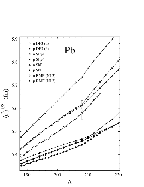
Figure 9: Root-mean-squared neutron (n, open symbols) and proton (p, solid symbols) radii for lead isotopes calculated with functional DF3 and parameter set (d) of the pairing force (4.5) (circles), in comparison with the Skyrme–HFB calculations for the forces SLy4 [75] (squares) and SkP [74] (triangles), and with the RMF–HBCS calculations [81] (diamonds). The big open circle with error bars shows the “experimental” rms neutron radius in ²⁰⁸Pb (see text).

It is of interest to compare the predictions obtained with different mean-field approaches not only for the proton radii but also for the neutron ones. An example is given in Fig. 9 where the results for the lead isotopes obtained with the functional DF3(d) are shown in comparison with the HFB+SkP and HFB+SLy4 calculations, and with recently published relativistic mean-field Hartree calculations [81] based on the effective force NL3 and the constant pairing gap prescription of Ref. [82] within the Bardeen-Cooper-Schriffer formalism (RMF–HBCS). It is seen that the EDF model with gradient pairing yields staggering in the evolution of the proton and neutron radii, and produces a kink in both of them at A=208. The Skyrme-type functionals produce very small kinks in proton radii. The calculations with the RMF–HBCS model are given in Ref. [81] for even-even nuclei only, but one would guess that this model is not able to produce noticeable odd-even staggering too. At the same time, as seen in Fig. 9, both Skyrme–HFB and the RMF–HBCS functionals predict bigger neutron radii than our EDF calculations, and all of them yield a distinctive kink in the evolution of $\langle r^{2}\rangle_{\rm n}$ at $A=208$. One observes rather close agreement between the proton radii obtained with all considered models but a wide spread in the neutron radii. The RMF–HBCS neutron radii are particularly large. We remark at this point that the “experimental” rms neutron radius in ²⁰⁸Pb of 5.593 fm deduced from the analysis of the high-energy polarized proton scattering in Ref. [83] is significantly lower than the prediction of the RMF(NL3) model; this fact has been already mentioned in Refs. [37, 84]. But one should bear in mind that the result of this analysis is model-dependent, and the errors in the extracted neutron radii could be quite large. The difference between neutron and proton rms radii for ²⁰⁸Pb, +0.14$\pm$0.04 fm, has been also deduced in Ref. [83], and we just put the corresponding error bars for the $\langle r^{2}\rangle_{n}^{1/2}$ value in this nucleus as shown in Fig. 9.

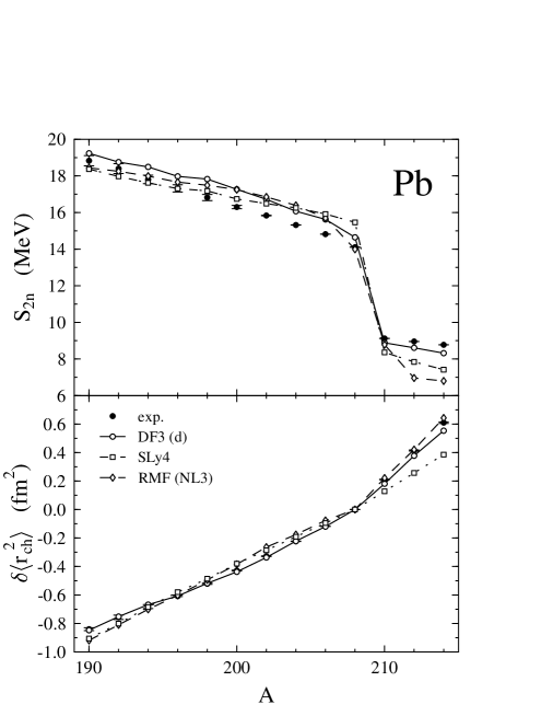
Figure 10: Two-neutron separation energies (upper panel) and differences of mean squared charge radii with respect to ²⁰⁸Pb (lower panel) for even lead isotopes. The open circles connected by the solid lines are obtained with functional DF3 and parameter set (d) of the pairing force (4.5). The open squares (diamonds) connected by the dotted (dashed) lines are from the Skyrme-SLy4 (RMF–HBCS) calculations. Solid circles: experimental data for $S_{2\rm n}$, including those derived from systematic trends, from [70], and data for $\delta\langle r^{2}_{\rm ch}\rangle$ from [71, 72, 73].

Considering general trends in the behavior of a given sequence of nuclei, we notice that, because of the strong pn attraction, the evolution of the proton radius should be driven by that of the neutron one through self-consistency, and vice versa. Moreover, in neutron-rich nuclei, an anticorrelation should exists between neutron radii and neutron separation energies: the larger $\langle r^{2}\rangle_{\rm n}$, the smaller $S_{2\rm n}$. One may suspect that too big neutron radii with a kink at $N=126$, which is correlated with a kink in proton radii, would mean too small $S_{2\rm n}$ values beyond the shell closure. This is indeed the case as clearly demonstrated in Fig. 10. This figure displays two-neutron separation energies $S_{2\rm n}$ (upper panel) and differences of mean square charge radii $\delta\langle r^{2}_{\rm ch}\rangle$ with respect to ²⁰⁸Pb (lower panel) for the even lead isotopes. The results obtained with the RMF(NL3), Skyrme-SLy4 and EDF-DF3(d) models are compared there with experiment. It is seen that all these models reproduce $S_{2\rm n}$ values for lighter Pb isotopes below $A=208$ fairly well, with more or less the same quality, the deviation from experiment being within 1 MeV or so (one should bear in mind that $S_{2\rm n}$ for the $A=190$–$198$ lead isotopes are derived in Ref. [70] from systematic trends, and the models discussed here describe these trends reasonable well). But for the heavier lead isotopes the predictions are different. Our EDF calculations with gradient pairing agree with experimental $S_{2\rm n}$ values within 0.5 MeV while Skyrme-SLy4 and RMF(NL3) models give deviations up to 1.5 and 2.0 MeV, respectively. It is also seen in the lower panel of Fig. 10 that the isotope shifts in charge radii for lighter Pb isotopes are nicely reproduced with our EDF approach, the $\delta\langle r^{2}_{\rm ch}\rangle$ values for the $A>208$ nuclei and the kink being slightly underestimated. The Skyrme-SLy4 and RMF(NL3) models work worse and yield results of equal quality for the lighter isotopes, but produce much different kinks and $\delta\langle r^{2}_{\rm ch}\rangle$ values beyond $A=208$. The kink obtained with the RMF model incorporating simple BCS pairing, with constant pairing gap, is impressive indeed, and good description of this anomaly in the isotope shifts of Pb nuclei has been reputed as a considerable success of the relativistic mean-field approach. The above consideration, which has much in common with that of Ref. [80], points out, however, the importance of simultaneous description of both physical quantities, i.e. the energetic ($S_{2\rm n}$) and geometrical ( $\delta\langle r^{2}_{\rm ch}\rangle$) differential observables, in order to get a deeper insight into the nature of this anomaly in the isotope shifts.

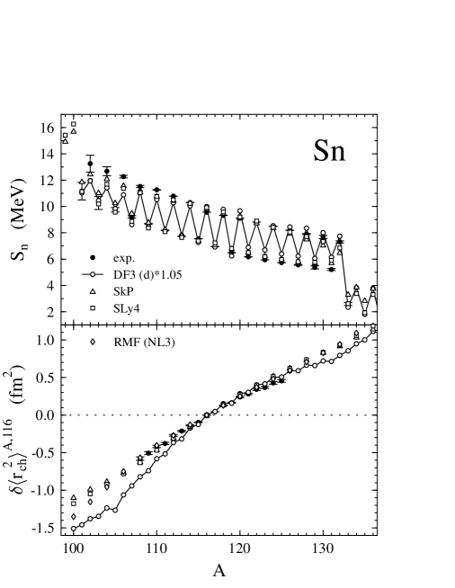
Figure 11: Neutron separation energies (top) and differences of mean square charge radii with respect to ¹¹⁶Sn (bottom) for tin isotopes. Open circles: EDF calculation with the set (d) of the pairing force, eq. (4.5). Open triangles (squares): Skyrme–HFB calculation with the force SkP (SLy4). In the lower panel, the open diamonds correspond to the RMF–HBCS $\delta\langle r^{2}_{\rm ch}\rangle$) values [81]. Solid circles: experimental data from [70] (for $S_{\rm n}$) and [85] (for $\delta\langle r^{2}_{\rm ch}\rangle$).

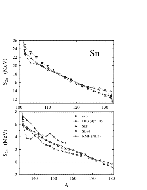
Figure 12: Two–neutron separation energies for even tin isotopes. Open circles: EDF–DF3 calculation with the set (d) of the pairing force, eq. (4.5), with a scaling factor of 1.05. Open triangles (squares): Skyrme–HFB calculation with the force SkP (SLy4). Open diamonds: RMF–HBCS calculation [81]. Solid circles: experimental data from [70].

The calculated neutron separation energies and differences of mean squared charge radii with respect to ¹¹⁶Sn for tin isotopes with mass number from A=99 to A=136 are shown in Fig. 11 in comparison with experimental data and with the Skyrme–HFB calculations based on the SkP and SLy4 forces. In the lower panel of this figure, we also show the RMF–HBCS $\delta\langle r^{2}_{\rm ch}\rangle$ values [81]. The results for radii from these three models are available for even isotopes only. Of the six parameter sets (4.5) of the pairing force, only the results for our preferable set (d), with a scaling factor of 1.05, are shown. Similar to the lead chain, the $S_{\rm n}$ values for tin isotopes are reproduced reasonably well. However, on both ends of the considered chain, near the magic nuclei ¹⁰⁰Sn and ¹³²Sn, the common trend for all mean-field calculations presented in the upper panel of Fig. 11 is that the size of the odd-even effect in neutron separation energies becomes noticeably smaller than the experimental one. As seen in the lower panel in Fig. 11, the evolution of the charge radii in the Skyrme-type and RMF–HBCS calculations is rather smooth, the SkP, SLy4 and RMF functionals slightly overestimate $\delta\langle r^{2}_{\rm ch}\rangle$ in the heavier tin isotopes above $A=120$. The desirable size of staggering in the behavior of $\delta\langle r^{2}_{\rm ch}\rangle$ for tin isotopes could be obtained with gradient pairing as shown by open circles in this figure. At the same time, the EDF calculations with functional DF3 significantly underestimate $\delta\langle r^{2}_{\rm ch}\rangle$ in lighter isotopes below A=114. This fact seems to be correlated with the weakening of the pairing when approaching A=100 and points out the need of both more careful adjustment of the normal isovector part of the energy-density functional and, probably, invoking the dependence of the pairing force on the isovector density $\rho_{-}=\rho_{\rm n}-\rho_{\rm p}$.

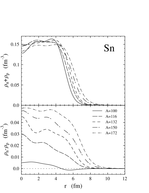
Figure 13: Isoscalar (top) and isovector (bottom) densities for some tin isotopes.

Figure 14: Neutron normal density (top), anomalous density (middle) and pairing gap (bottom) in three selected tin isotopes.

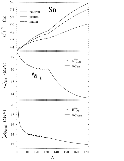
Figure 15: Neutron, proton and matter rms radii (top), mean energy of isovector dipole (middle) and Fermi charge-exchange (bottom) transitions for tin isotopes. The solid dots for $\langle\omega\rangle_{\rm dip}$ correspond to the experimental data for the maximum of the dipole photoabsorption Lorentz curves, Refs. [86, 87], while those for $\langle\omega\rangle_{\rm Fermi}$ to the experimental positions of the isobaric analog states with respect to the daughter nuclei, Ref. [88].

The calculated two–neutron separation energies for even tin isotopes up to the neutron drip line are shown in Fig. 12. Again, the set (d) of the pairing force with a scaling factor of 1.05 was used in the EDF calculations with the parametrization DF3. One can observe noticeable differences between the Skyrme–HFB calculations with the SkP and SLy4 forces, the RMF–HBCS predictions, and the EDF results. The RMF-HBCS calculations [81] are performed with deformed code, and available for the tin isotopes only up to $A=156$; these calculations produce some irregularities in the $S_{2\rm n}$ values near $A=100$ and $A=132$ (the nuclei beyond ¹⁴⁰Sn are predicted to be well deformed). At the same time, the three other spherical microscopic calculations give surprisingly similar predictions when approaching the neutron drip line, the heaviest bound tin nucleus being ¹⁷²Sn, ¹⁷⁴Sn and ¹⁷⁶Sn for the EDF, SkP and SLy4, respectively. One should notice that the Skyrme–HFB calculations were performed with a discretized continuum in a spherical box of finite size [74] which allows to artificially obtain a stable solution for the nuclear ground state even for positive value of the chemical potential. Such a solution is not possible with the coordinate-space technique used in the present paper because of the physical boundary conditions imposed for the scattering states.

The evolution of the isoscalar and isovector densities along the tin isotope chain is illustrated in Fig. 13. It is seen that isovector density $\rho_{-}=\rho_{\rm n}-\rho_{\rm p}$ increases both in the volume and at the surface as the neutron number $N$ becomes larger. The isoscalar (matter) density tends to be slightly decreased with $N$ in the volume and became more diffused at the surface. The matter distributions in the two magic nuclei, ¹⁰⁰Sn and ¹³²Sn, have a steeper slope at the surface compared to the non-magic isotopes. The radial dependence of the neutron pairing field $\Delta(r)$, of the anomalous density $\nu(r)$ and of the normal neutron density $\rho_{\rm n}(r)$ for the stable nucleus ¹¹⁶Sn, for the unstable isotope ¹⁵⁰Sn and for the drip-line nuclide ¹⁷²Sn are shown in Fig. 14. One can see that in the heavier isotopes, the anomalous density becomes more diffuse at the surface with a longer tail compared to the normal densities, in agreement with the discussion given in Appendix C. It is also seen that the pairing field $\Delta$ in the outer part of the nuclear surface has a prominent maximum which moves outwards and gets a larger tail near the drip line. The concentration of $\Delta$ outside of the half density point is related to the specific cancellation between the external attraction and the repulsive gradient term in the effective pairing force [24].

The staggering phenomenon observed in the behavior of charge radii plotted as a function of neutron number is the one of the prominent odd-even effects which has been systematically measured and widely discussed. Similar effects are expected to exist for other quantities such as neutron and matter radii, centroid energies of multipole excitations (position of the giant resonances), etc.

Shown in the upper panel of Fig. 15 are the root-mean-square proton, neutron and matter radii for the tin isotope chain calculated with the functional DF3 and with the set (d) of the pairing force. In the middle panel of this figure we show the mean energies $\langle\omega\rangle_{\rm dip}$ of dipole isovector excitations. These are calculated as the square root of the ratio $m_{3}/m_{1}$ with $m_{1}$ and $m_{3}$ the linear and cubic energy-weighted sum rule, i.e. the first and the third moment of the corresponding RPA strength distribution, respectively [89]:

$$\langle\omega\rangle_{\rm dip}=\left[-{{\hbar^{2}}\over{3m}}{A\over{NZ}}\int\d\vec{r}\d\vec{r}\,^{\prime}\,{{\partial\rho_{\rm n}}\over{\partial\vec{r}}}{\mathcal{F}}^{\rm np}(\vec{r},\vec{r}\,^{\prime}){{\partial\rho_{\rm p}}\over{\partial\vec{r}\,^{\prime}}}\right]^{1/2}\,.$$ (5.1)

Here ${\mathcal{F}}^{\rm np}$ is the effective neutron–proton interaction obtained from the energy-density functional as the second variational derivative $\delta^{2}E_{\rm int}/\delta\rho_{\rm n}\delta\rho_{\rm p}$. In the lower panel of Fig. 15 we show the mean energies $\langle\omega\rangle_{\rm Fermi}$ of the charge-exchange $0^{+}$ excitations, i.e. the Fermi transitions, in tin nuclei with $N>Z$. These energies are calculated within the sum rule approach as the ratio $(m_{1}^{+}+m_{1}^{-})/(m_{0}^{+}-m_{0}^{-})$ with $m_{1}^{+}$ and $m_{1}^{-}$ the first moment of the strength distribution of the Fermi transitions in the $\beta^{+}$ and $\beta^{-}$ channel, respectively (energy-weighted sum rules) and with $m_{0}^{+}$ and $m_{0}^{-}$ the corresponding non-energy weighted sum rules. The resulting expression for $\langle\omega\rangle_{\rm Fermi}$ is given by (see, for example, [90]):

$$\langle\omega\rangle_{\rm Fermi}={1\over{N-Z}}\int\d\vec{r}\,U_{\rm Coul}(\vec{r})\left(\rho_{\rm n}(\vec{r})-\rho_{\rm p}(\vec{r})\right)\,,$$ (5.2)

where $U_{\rm Coul}$ is the Coulomb mean field potential.

It is seen in Fig. 15 that the rms neutron, proton and matter radii as functions of the mass number $A$ reveal a kink at magic ¹³²Sn, and at larger $A$ the difference between rms neutron and proton radii starts to increase more rapidly. The staggering in radii is present mostly in the region between the two magic nuclei, from ¹⁰⁰Sn to ¹³²Sn, and this effect is practically washed out beyond $A=140$. The mean energy of dipole transitions occurs to be in anticorrelation with such a behavior in radii, and this seem to be in qualitative agreement with experimental data (one should mention that eq. (5.1) overestimates the position of the giant dipole resonance by $\approx 0.5$ MeV because of the cubic energy-weighted sum rule $m_{3}$ used in the derivation of $\langle\omega\rangle_{\rm dip}$). One also observes a distinct kink in the behavior of $\langle\omega\rangle_{\rm dip}$ at $A=132$. Beyond this magic number the mean dipole energy decreases rather fast and then nearly saturates when approaching $A=172$. This might be connected with an enhancement of the low-energy dipole transitions [91] and also with possible appearance of the so-called soft dipole mode [92] in nuclei near the neutron drip line. The anticorrelations in the staggering behavior of $\langle\omega\rangle_{\rm dip}$ and the rms radii $\langle r^{2}\rangle^{1/2}_{\rm n}$, $\langle r^{2}\rangle^{1/2}_{\rm p}$ can easily be understood by considering the influence of pairing on the gradients of neutron and proton densities entering eq. (5.1). The odd-even effect in $\langle\omega\rangle_{\rm dip}$ is constructive and more pronounced in the $A\leq 132$ region where both gradients strongly overlap. Beyond ¹³²Sn, the larger differences between neutron and proton rms radii imply lower overlap between neutron and proton density gradients at the nuclear surface, hence a smaller mean dipole energy. The situation with mean energy of the Fermi charge-exchange transitions is different. From eq. (5.2) one expects that the correlation between $\langle\omega\rangle_{\rm Fermi}$ and the neutron and proton rms radii should be destructive. As seen in the lower panel in Fig. 15, the staggering in the evolution of $\langle\omega\rangle_{\rm Fermi}$ with $A$ is very weak indeed and almost invisible. The kink at the magic mass number $A=132$ is also much less pronounced compared to the dipole case. Remarkable enough, the theoretical self-consistent sum-rule predictions for $\langle\omega\rangle_{\rm Fermi}$ in tin isotopes are in excellent agreement with the available experimental data on the position of the isobaric analog states.

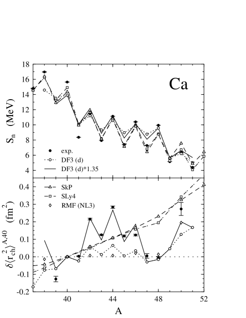
Figure 16: Neutron separation energies (top) and differences of mean squared charge radii with respect to ⁴⁰Ca (bottom) for calcium isotopes. Open circles: the EDF calculation with the set (d) of the pairing force, eq. (4.5). Solid lines connect the EDF results also obtained for the set (d) but with a scaling factor of 1.35. Open triangles (squares): Skyrme–HFB calculation with the force SkP (SLy4). In the lower panel, the open diamonds correspond to the RMF–HBCS $\delta\langle r^{2}_{\rm ch}\rangle$ values [81] (for even isotopes only). Solid circles: experimental data from [70] (for $S_{\rm n}$) and [93, 94, 95] (for $\delta\langle r^{2}_{\rm ch}\rangle$).

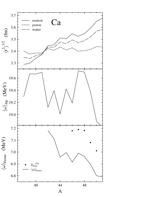
Figure 17: Neutron, proton and matter radii (top), mean energy of isovector dipole (middle) and Fermi charge-exchange (bottom) transitions for calcium isotopes. The solid dots for $\langle\omega\rangle_{\rm Fermi}$ correspond to the experimental positions of the isobaric analog states with respect to the daughter nuclei, Ref. [88].

Fig. 16 displays the neutron separation energies and isotope shifts in mean square charge radii for the calcium isotope chain. In this case, the EDF calculations with the preferable set (d), eq. (4.5), deduced from the Pb isotopes yield noticeable but rather small staggering both in $S_{\rm n}$ and $\delta\langle r^{2}_{\rm ch}\rangle$. A possible way to get the desirable size of odd-even effects is to enhance the pairing correlations by introducing a scaling factor 1.35 for the pairing force (all parameters being scaled in the same way). It is seen then in Fig. 16 that the neutron separation energies are reproduced fairly well, with more or less the same quality as with the Skyrme SkP and SLy4 functionals, though the effect of the scaling is rather mild. The effect on the behavior of charge radii is more drastic: the $\delta\langle r^{2}_{\rm ch}\rangle$ values are increased by a factor of 3 to 4 yielding a very good agreement with experiment. This example demonstrates that the anomalous $A$-dependence of charge radii in Ca isotopes could be correctly described within the EDF approach with renormalized pairing force. However, the possibility to determine a single parametrization of the effective interaction in the pp channel, which would be valid both for heavy and light nuclei, remains an open problem. In any case, we got an indication that the staggering in $\delta\langle r^{2}_{\rm ch}\rangle$ of Ca isotopes, which is a challenge for nuclear models, could be explained with a peculiar density dependence of the pairing force. One can see in Fig. 16 that the Skyrme SkP and SLy4 functionals produce a nearly smooth increase of radii with $A$, with weak irregularities below and above $A=48$, but still with rather sizeable kinks at double magic ⁴⁸Ca. The RMF–HBCS predictions for $\delta\langle r^{2}_{\rm ch}\rangle$, Ref. [81], are much different: the charge radius is nearly a constant up to ⁴⁸Ca, with a sudden increase for ⁵⁰Ca. Interestingly, the functional DF3 yields, in agreement with experiment, a small negative isotope shift in charge radii between ⁴⁰Ca and ⁴⁸Ca, which does not depend on pairing.

The EDF calculations, as demonstrated in Fig. 17, show that the trends and the staggering effects in the mean energy of isovector dipole excitations and charge-exchange Fermi transitions for calcium isotopes are in strong anticorrelation with evolution of the ground state mean squared radii. Similar to the case of the tin isotopes discussed above, the anticorrelation in $\langle\omega\rangle_{\rm Fermi}$ is weaker than in $\langle\omega\rangle_{\rm dip}$. Unfortunately, there are no systematic experimental data on dipole excitations in Ca isotopes at our disposal, from which the $\langle\omega\rangle_{\rm dip}$ values could be deduced. As for the mean energies of the Fermi transitions, which are calculated with the self-consistent EDF sum rule approach and plotted as a function of $A$ in the lower panel in Fig. 17, they may be compared with the experimental positions of the isobaric analog states. It is seen that the sum rule expression, eq. (5.2), underestimates the energy of the analog states in calcium isotopes by some 200 keV but reproduces qualitatively the observed trend.

As, in the past, RPA ground state correlations have been invoked to explain details of the isotopic dependence of nuclear charge radii, we estimate the influence of RPA ground state correlations.

6 Ground state fluctuations

An important point is the issue of RPA-type ground state correlations. In several papers [72, 96, 97] the influence of the average mean square deformations on the mean square charge radii has been discussed in a phenomenological way which is based on the following sum rule: Take the identity for the multipole operator $Q_{\lambda,\mu}=\int\d{\vec{r}}r^{\lambda}Y_{\lambda,\mu}(\Omega)\psi^{\dagger}({\vec{r}})\psi({\vec{r}})$

$$\sum_{\mu}\langle 0|\;|Q_{\lambda,\mu}|^{2}|0\rangle=\sum_{\mu,s}|\langle s|Q_{\lambda,\mu}|0\rangle|^{2}\;.$$ (6.1)

The right hand side is equal to the summed transition strength $\sum_{s}\!B({\rm E}\lambda;\!{0\!\!\to\!\!s})$, the left hand side is the expectation value of the squared multipole operator $Q_{\lambda}$ in the ground state. In semiclassical nuclear models, this expectation value is proportional to the square of the deformation of multipolarity $\lambda$. Thus, even for spherical nuclei the rms deformation does not vanish. In the liquid drop model this is interpreted as due to zero point surface vibrations, but it is to be emphasized that there is no observable time dependence, and no breaking of the spherical symmetry due to this “dynamical” deformation. Experimentally, the effect can not be distinguished from diffuseness of the surface arising from any other mechanism.

Our method (as well as any HF or HFB calculation) incorporates only the dynamical deformation effects corresponding to a gas of noninteracting particles (magic nuclei) or of a gas with only pairing (nonmagic nuclei). To include the RPA ground state correlations, the calculated charge radii should be increased by

$$\delta\langle r_{\rm ch}^{2}\rangle=\bar{\delta}\langle r_{\rm ch}^{2}\rangle_{\rm RPA}-\bar{\delta}\langle r_{\rm ch}^{2}\rangle_{\rm HFB}.$$ (6.2)

However, the parameters have been adjusted to reproduce the experimental density distribution and therefore the average RPA correlations are included due to the choice of parameters. In a high precision fit, this should be corrected for, by subtracting the value given by (6.2) for the reference nucleus.

A microscopic method to calculate the corrections to $\langle r^{2}_{\rm ch}\rangle$ due to low-energy surface vibrations has been proposed in [98]. We use the liquid drop model and eq. (6.1) to estimate the influence of isoscalar collective excitations on the charge radii, as proposed by Esbensen and Bertsch [96].

As already noted in [96], the inclusion of noncollective states in eq. (6.1), which can not be considered to be surface oscillations will not do much harm, because the contribution of these states will be essentially the same to $\bar{\delta}\langle r^{2}_{\rm ch}\rangle_{\rm RPA}$ and $\bar{\delta}\langle r^{2}_{\rm ch}\rangle_{\rm HFB}$ and will drop out. According to [72, 99, 100], for multipolarity $\lambda>0$

$$\bar{\delta}\langle r^{2}_{\rm ch}\rangle\equiv\langle r^{2}\rangle_{\rm d}-\langle r^{2}\rangle_{\rm s}={5\over{4\pi}}\langle r^{2}\rangle_{\rm s}\sum_{\lambda}\langle\beta_{\lambda}^{2}\rangle\,,$$ (6.3)

where the suffixes d and s mean (dynamically) deformed and spherical, respectively.

Within the same model

$$S^{0}({\rm E}\lambda)\equiv\sum_{s}B(E\lambda;0\!\rightarrow\!s)=\sum_{\mu}\langle 0|\;|Q_{\lambda,\mu}|^{2}|0\rangle=\left({{3ZeR_{0}^{\lambda}}\over{4\pi}}\right)^{2}\langle\beta_{\lambda}^{2}\rangle\,.$$ (6.4)

With the help of (6.4) and (6.1) the sum over $\beta_{\lambda}^{2}$ in eq. (6.3) can be replaced by the sum over the total $B({\rm E}\lambda)$-values, and we reach the following expression:

$$\delta\langle r_{\rm ch}^{2}\rangle={{4\pi}\over{3Z^{2}e^{2}}}\sum_{\lambda}{1\over{R_{0}^{\lambda-2}}}[S_{\rm RPA}^{0}({\rm E}\lambda)-S_{\rm HFB}^{0}({\rm E}\lambda)]\,.$$ (6.5)

Of course, for $\lambda=1$ one has to exclude the spurious translation. For $\lambda=0$ we have to use a compressible drop model, and obtain similarly

$$\delta\langle r_{\rm ch}^{2}\rangle={{140\pi}\over{108Z^{2}e^{2}R_{0}^{2}}}[S_{\rm RPA}^{0}({\rm E}0)-S_{\rm HFB}^{0}({\rm E}0)]\,.$$ (6.6)

where $S({\rm E}0)$ is calculated according to eq. (6.4) with $Q_{00}=r^{2}Y_{00}$.

Table 1.

Excitation energies (MeV) and transition probabilities $(e^{2}~{}\cdot$fm${}^{2L})$ for low-lying collective states. Experimental data are taken from Refs. [102, 103] (for Ca), [104] (for Sn) and [105] (for Pb).

Isotope exp for $$2^{+}_{1}$$ theory for exp for theory for

B(E2) B(E2) B(E3) B(E3)

⁴⁰Ca - - - - 3.74 3.79

⁴²Ca 1.53 3.15 3.45 4.47

⁴⁴Ca 1.16 3.00 3.31 4.70

⁴⁶Ca 1.35 2.22 3.61 4.73

⁴⁸Ca 3.83 3.18 4.51 4.46

¹⁰⁰Sn - - 4.34 - - 6.00

¹⁰⁸Sn 1.21 1.76 3.70

¹¹²Sn 1.26 1.73 2.35 3.36

¹¹⁶Sn 1.29 1.71 2.27 3.17

¹²⁰Sn 1.17 1.67 2.40 3.24

¹²⁴Sn 1.13 1.74 2.62 3.49

¹³²Sn - - 4.32 4.04 - 4.94

¹⁹⁰Pb - - 1.31 - - 2.43

²⁰⁰Pb 1.03 1.23 3.01

²⁰⁴Pb 0.90 1.24 2.61 3.14

²⁰⁶Pb 0.80 1.20 2.65 3.14

²⁰⁸Pb 4.08 4.87 2.61 3.00

²¹⁰Pb 0.80 1.29 1.87 2.42

²¹²Pb 0.81 1.32 1.82 2.17

Table 2.

$\delta\langle r^{2}_{\rm ch}\rangle$ (in fm²) for different multipolarities for ⁴⁰Ca, ⁴⁴Ca, and ⁴⁸Ca isotopes calculated within the framework of self consistent QRPA.

$$J^{\pi} \delta\langle r^{2}_{\rm ch}\rangle 0^{+} 2^{+} 3^{-} 4^{+} \sum_{2^{+},3^{-}} \sum_{\rm tot}$$ ⁴⁰Ca ⁴⁴Ca ⁴⁸Ca -0.0062 -0.0046 -0.0043 0.0322 0.0597 0.0278 0.2604 0.1463 0.0432 0.0111 0.0149 -0.0293 0.2926 0.2060 0.0710 0.2975 0.2163 0.0374

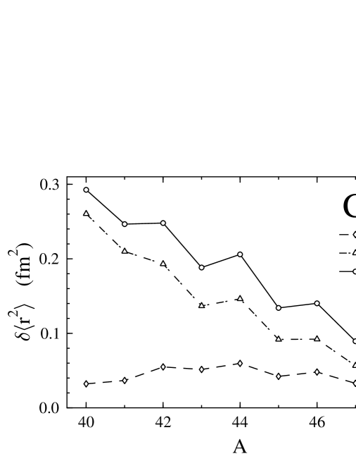
Figure 18: Contribution of RPA ground state correlations to the squared charge radii in calcium isotopes. Shown are the $2^{+}$ (diamonds) and the $3^{-}$ (triangles) contributions and the sum of both (circles). It is seen that ⁴⁰Ca is quite soft for 3^- deformation and gets a big contribution from the corresponding ground state fluctuations.

The excited states have been calculated in quasiparticle-RPA (QRPA) which has been used in the form (we adopt the same symbolic notations as in Ref. [10]):

$$\hat{V}=e_{q}\hat{V}_{0}+\hat{F}\hat{A}\hat{V}\,,\quad S_{\rm RPA}^{0}=-{1\over\pi}{\rm Im}(e_{q}\hat{V}_{0}\hat{A}\hat{V})\,,$$ (6.7)

where $e_{q}$ is the quasiparticle local charge with respect to the external field $V_{0}$. For a long-range electric field, $V_{0}\propto Q_{\lambda,\mu}$, from gauge invariance one gets $e_{q}=1$ [10]. The $\hat{A}$ matrix is written in detail in [101].

As in our formalism the effective interaction amplitudes $\hat{F}$ are obtained as the second functional derivatives of $E_{\rm int}$ with respect to the corresponding densities, one can see here that due to $\rho$-dependence of $\varepsilon_{\rm anomal}$, eq. (4.1), there are mixed terms for the effective interaction, $F^{\omega\xi}$ and $F^{\xi\omega}$, which do not vanish, and which couple the ph with the pp or hh channel ($\tau$-indices are neglected for simplicity):

$${\mathcal{F}}^{\omega\xi}={{\textstyle\delta^{2}E_{\rm int}[\rho,\nu]}\over{\textstyle\delta\rho\delta\nu}}={{\delta^{2}}\over{\delta\rho\delta\nu}}\int\varepsilon_{\rm anomal}([\rho,\nu];\vec{r})\d\vec{r}\,,$$ (6.8)

A comparison of QRPA results for the first collective $2^{+}$ and $3^{-}$ states with experiment is presented in Table 1 for selected nuclei from the Ca, Sn and Pb isotope chains. The influence of the spin–orbit part in the ph interaction has been investigated in [21]; the results given here have been obtained without this spin–orbit contribution. Comparison with [21] shows that here the changes in the functional did not improve the agreement with experimental data.

Figure 19: The same as Fig. 18, for selected isotopes from the tin chain.

Figure 20: The same as Fig. 19 for lead.

We restricted our consideration to $2^{+}$ and $3^{-}$ states for all isotope chains because the other multipolarities contribute much less to the mean square charge radii [98]. This has been checked by computing also $\delta\langle r^{2}_{\rm ch}\rangle$ from $0^{+}$ and $4^{+}$ states for three calcium isotopes. In all these calculations the functional parameter set of Ref. [22] have been used. These results are presented in Table 2 in comparison with the calculations for $2^{+}$ and $3^{-}$ multipolarities. One can see a here significant difference between $2^{+}$ and $3^{-}$ states on one hand and $0^{+}$ and $4^{+}$ states on the other hand. Therefore it is sufficient to include only strong phonons which contribute significantly to the mean square radii. This result is very similar to that of Barranco and Broglia [97] which they obtained with the approach of Esbensen and Bertsch [96] for the calculation of $\delta\langle r^{2}_{\rm ch}\rangle$ values. However, it should be mentioned that they used a non self consistent model with more freedom in the choice of parameters.

Let us now look at the results of our calculation for the calcium, tin and lead isotope chains which are presented in Figs. 18, 19, and 20, respectively. One can see here that for calcium isotopes $3^{-}$ states give the main contribution to $\delta\langle r^{2}_{\rm ch}\rangle_{\rm tot}$, especially for ⁴⁰Ca (Fig. 18). The $2^{+}$ contribution is not very big, in contrast to the result of [97]. This is connected with the fact that we could not obtain the experimental values for excitation energies and especially for $B({\rm E}2)$ values in calcium isotopes in the middle of the chain. Presumably for good reproduction of the experimental values one has to go beyond the QRPA in a model which allows to take into account more complex configurations than 1p1h. Nevertheless, it is shown that there is considerable influence of ground state correlations on the calcium mean square charge radii, at least in second order in the phonon amplitudes. Combining the EDF results shown in Fig. 18 with those in Fig. 16 one sees that the staggering in charge radii of calcium isotopes could be enhanced by the calculated ground state correlation corrections; however, this would produce too big negative isotope shift between ⁴⁰Ca and ⁴⁸Ca thus deteriorating the good agreement with experiment seen in Fig. 16 alone.

In Figs. 19 and 20 the ground state correlation contribution to $\delta\langle r^{2}_{\rm ch}\rangle$ is shown for a few isotopes of the tin and lead chains. These nuclei are more stiff, and QRPA works much better (see Table 1). The results show that here the ground state correlation contribution is only a small fraction of the value obtained without correlations. Moreover, the general trends look roughly like the trends of the curves for $\delta\langle r^{2}_{\rm ch}\rangle$ from Figs. 5, 6 and 11, which therefore are enhanced but not qualitatively changed by the correlations.

7 Summary and conclusions

In this work the energy density functional method for superfluid nuclei has been described in detail. The generalized variational principle has been formulated for the local functional with a contact effective force ${\mathcal{F}}^{\xi}$ in the particle–particle channel and cutoff energy $\epsilon_{\rm c}\geq\epsilon_{\rm F}$. For spherical finite systems, the coordinate-space technique, involving the integration in the complex energy plane of the Green’s functions obtained by solving the Gor’kov equations exactly, with physical boundary conditions both for bound and scattering quasiparticle states has been used. The technique has been extended to odd nuclei by using a uniform filling approximation.

Within the framework of this EDF approach, the combined analysis of differential observables including odd-even mass differences and odd-even effects in charge radii was performed for a few isotopic chains. The staggering and kinks in $\delta\langle r^{2}_{\rm ch}\rangle$ were shown to be very sensitive to the density dependence of the effective pairing force. The observed isotopic shifts were successfully described with the force containing a density-gradient pairing term. With such a parametrization, as the external attraction $\propto f^{\xi}_{\rm ex}$ increases, the pairing field $\Delta(r)$ becomes smaller in the volume and concentrates in the outer part of the nuclear surface.

A few possible parameter sets extracted from the lead chain were used to study the ground state properties of uniform nuclear matter with $s$-wave pairing, in particular the behavior of the energy gap at the Fermi level as a function of density. The deduced sets, which give a satisfactory description of both the neutron separation energies $S_{\rm n}$ and isotope shifts $\delta\langle r^{2}_{\rm ch}\rangle$ in charge radii, yielded about the same value of $\Delta\approx 3.3$ MeV at $k_{\rm F}=1.15$ fm^-1 (at $\approx 0.65$ of the equilibrium density). It was found that some sets in the dilute limit correspond to the strong coupling regime. The situation when the regime changes from weak to strong pairing was considered in detail, and, in strong coupling, the properties of dilute matter were shown to be completely determined in leading order by the singlet scattering length $a_{\rm nn}$. In weak coupling, near gap closure, the pairing gap $\Delta_{\rm F}$ is shown to be directly expressed through the Fermi level phase shifts. The density-dependent cutoff contact pairing interaction corresponding to the realistic value of the singlet NN scattering length was found to be a preferable choice between the deduced parameter sets to be used in the EDF calculations.

The isotopic chain of tin isotopes from the proton to the neutron drip line was calculated, and the evolution of the normal and anomalous (pairing) density distributions with $A$ was analyzed. The parametrization DF3 of the normal part of the functional and the density-dependent pairing interaction provided fairly good description of odd-even effects in $S_{\rm n}$ and $\delta\langle r^{2}_{\rm ch}\rangle$; however, in the region of lighter tin isotopes the slope in $\delta\langle r^{2}_{\rm ch}\rangle$ plotted as a function of the mass number $A$ come out steeper than in experiment. This might indicate that dependence on isovector density $\rho_{-}=\rho_{\rm n}-\rho_{\rm p}$ should be incorporated in the effective pairing interaction. Anomalous behavior of charge radii in Ca isotopes was reproduced in excellent agreement with experiment within the EDF approach by scaling the pairing effective interaction which was extracted from the lead chain by a factor of 1.35.

It was shown with the self-consistent sum rule approach that the density-dependent pairing induces sizeable staggering and kinks in the evolution of the mean energies of multipole excitations along isotopic chains. These effects were found to be in anticorrelation with the behavior of the ground state radii.

Using quasiparticle-RPA multipole strength distributions obtained with the self-consistent interaction, the contribution of phonons (ground state correlations) to the differences of charge radii was calculated by the method proposed by Esbensen and Bertsch [96]. It was shown that these phonon corrections, at least for tin and lead isotopes, are quite small in comparison with the values provided by the main HFB contribution, and do not lead to qualitatively new effects.

The results obtained in the present paper were compared with the conventional Skyrme–HFB, Gogny–HFB and relativistic mean field Hartree-BCS calculations. On the whole, a better description of the differential observables was achieved with the EDF method, the most important effect which was successfully reproduced is the staggering in charge radii. Up to now, this effect was practically missed in all other mean-field models. The famous kink in the isotope shifts of Pb isotopes has been also well described by our EDF calculations, with density-dependent gradient pairing, and the crucial point is that the neutron separation energies are reproduced as well. These results support the conclusion drawn by Reinhard and Flocard [80] that this is apparently not the case in the RMF model. These authors showed that the description of the kink in Pb chain is not proprietary to the relativistic model, it can be also produced with the Skyrme functionals by generalizing the spin-orbit term. However, even with their “best” set SkI4, Reinhard and Flocard have found a large gap in the single-particle neutron spectrum similar to that of the RMF model. Our conclusion is that the physics behind the anomaly in the Pb radii is not solely due to the spin-orbit (which, moreover, has nothing to do with the staggering!), and that the simultaneous reproduction of both the energetic and geometrical observables is important to settle the problem.

Unfortunately, a universal parametrization of the pairing force is still lacking, and for various isotope chains, especially for lighter nuclei, the parameters of ${\mathcal{F}}^{\xi}$ had to be chosen somewhat different. It seems to be necessary to use a more refined parametrization, e.g. with additional dependence of ${\mathcal{F}}^{\xi}$ on $\rho_{-}$. Also, more attention should be payed to the normal part of the density functional in order to choose more carefully its parameters and improve the description of the bulk properties of nuclei such as their masses and absolute values of radii [106, 107]. These questions will be investigated in future work.

Appendix A. General variational principle and ground state energy in local approximation

In this appendix we show that, in the case of weak pairing $|\Delta|\ll\epsilon_{\rm F}$, the general variational principle for a local density functional with an energy cutoff $\epsilon_{\rm c}>\epsilon_{\rm F}$ can be used to describe the ground state properties of superfluid systems. This allows to perform a full HFB-like calculation with a renormalized gap equation and an effective pairing $\delta$-force.

We start with the usual definitions and equations which follow from the general variational principle. The total energy $E$ of a superfluid system, as given by eqs. (2.10)–(2.12), is a functional of the generalized one-body density matrix $\widehat{R}$. This matrix can be expressed in terms of the ground state expectation values of the pair products of the Landau-Migdal quasiparticle creation and annihilation operators $\psi^{\dagger},\;\psi$:

$${\widehat{R}}(1,2) = \left(\matrix{\langle\psi^{\dagger}(2)\psi(1)\rangle&\langle\psi(2)\psi(1)\rangle\cr\langle\psi^{\dagger}(2)\psi^{\dagger}(1)\rangle&\langle\psi(2)\psi^{\dagger}(1)\rangle\cr}\right)$$ (A.1)

$$= \left(\matrix{\rho(1,2)&\nu(1,2)\cr-\nu^{*}(1,2)&\delta(1,2)-\rho^{*}(1,2)\cr}\right)\,.$$

Here the coordinate space representation is used. The numbers in brackets stand for the set of all relevant arguments and indices, e.g. $(1)=(\{\vec{r},s_{z},\tau_{3}\}_{1})$. In the following, $\int\d 1$ means integration over the continuous and summation over the discrete variables of this set.

The Bogolyubov quasiparticle creation and annihilation operators $\beta^{\dagger}_{\alpha}$, $\beta_{\alpha}$ are defined by the transformation

$$\left(\begin{array}[]{c}\beta_{\alpha}\\ \beta^{\dagger}_{\alpha}\end{array}\right)=\int\d 1\left(\begin{array}[]{cc}U^{*}_{\alpha}(1)&V^{*}_{\alpha}(1)\\ V_{\alpha}(1)&U_{\alpha}(1)\end{array}\right)\left(\begin{array}[]{c}\psi(1)\\ \psi^{\dagger}(1)\end{array}\right)\,.$$ (A.2)

This can be inverted to express the Landau-Migdal quasiparticle operators in terms of those of Bogolyubov

$$\left(\begin{array}[]{c}\psi(1)\\ \psi^{\dagger}(1)\end{array}\right)=\sum_{\alpha}\left(\begin{array}[]{cc}U_{\alpha}(1)&V^{*}_{\alpha}(1)\\ V_{\alpha}(1)&U^{*}_{\alpha}(1)\end{array}\right)\left(\begin{array}[]{c}\beta_{\alpha}\\ \beta^{\dagger}_{\alpha}\end{array}\right)\,.$$ (A.3)

The generalized Bogolyubov quasiparticle density matrix $\widehat{Q}$ is given by

$${\widehat{Q}}_{\alpha\alpha^{\prime}}=\left(\matrix{\langle\beta^{\dagger}_{\alpha^{\prime}}\beta_{\alpha}\rangle&\langle\beta_{\alpha^{\prime}}\beta_{\alpha}\rangle\cr\langle\beta^{\dagger}_{\alpha^{\prime}}\beta^{\dagger}_{\alpha}\rangle&\langle\beta_{\alpha^{\prime}}\beta^{\dagger}_{\alpha}\rangle\cr}\right)\;.$$ (A.4)

By demanding now the ground sate $|\Phi_{0}\rangle$ to be the Bogolyubov quasiparticle vacuum, $\beta_{\alpha}|\Phi_{0}\rangle=0$, the matrix $\widehat{Q}$ becomes diagonal in the $\alpha$–representation:

$${\widehat{Q}}_{\alpha\alpha^{\prime}}=\delta_{\alpha\alpha^{\prime}}Q\,,\quad{\rm with}\quad Q=\left(\begin{array}[]{cc}0&0\\ 0&1\end{array}\right)\,,$$ (A.5)

and for (A.1) one obtains a “supermatrix” formula:

$${\widehat{R}}(1,2)=\sum_{\alpha\alpha^{\prime}}{\mathcal{W}}_{\alpha}(1){\widehat{Q}}_{\alpha\alpha^{\prime}}{\mathcal{W}}^{\dagger}_{\alpha^{\prime}}(2)=\sum_{\alpha}{\mathcal{W}}_{\alpha}(1)Q{\mathcal{W}}^{\dagger}_{\alpha}(2)\,,$$ (A.6)

with the matrix ${\mathcal{W}}$ of the Bogolyubov transformation (A.3):

$${\mathcal{W}}_{\alpha}(1)=\left(\begin{array}[]{cc}U_{\alpha}(1)&V^{*}_{\alpha}(1)\\ V_{\alpha}(1)&U^{*}_{\alpha}(1)\end{array}\right)\,.$$ (A.7)

For the generalized density matrix we thus find

$${\widehat{R}}(1,2)=\sum_{\alpha}\left(\matrix{V_{\alpha}^{*}(1)V_{\alpha}(2)&V_{\alpha}^{*}(1)U_{\alpha}(2)\cr U_{\alpha}^{*}(1)V_{\alpha}(2)&U_{\alpha}^{*}(1)U_{\alpha}(2)\cr}\right)\,.$$ (A.8)

The matrix ${\mathcal{W}}$ obeys the generalized closure and orthogonality relations:

$$\sum_{\alpha}{\mathcal{W}}_{\alpha}(1){\mathcal{W}}^{\dagger}_{\alpha}(2)=\left(\begin{array}[]{cc}1&0\\ 0&1\end{array}\right)\delta(1,2)\equiv{\hat{I}}\delta(1,2)\,,$$ (A.9)

$$\int\d 1{\mathcal{W}}^{\dagger}_{\alpha}(1){\mathcal{W}}_{\alpha^{\prime}}(1)={\hat{I}}\delta_{\alpha\alpha\prime}\,.$$ (A.10)

The generalized density matrix $\widehat{R}$ is Hermitian and from eqs. (A.5–A.10) follows its important property (2.15) which, in the coordinate space representation, reads

$$\int\d 3{\widehat{R}}(1,3){\widehat{R}}(3,2)={\widehat{R}}(1,2)\,.$$ (A.11)

This property reflects the fact that the ground state is a HFB quasiparticle vacuum.

Minimizing the energy and imposing the average particle number conservation (2.14) and the relation (A.11) as constraints, we arrive at the variational principle $\delta I[\widehat{R}]=0\,$ with the variational functional of eq. (2.16) which we rewrite here as

$$I[\widehat{R}]=E[\widehat{R}]-\mu{\rm Tr}{\hat{\rho}}-{\rm Tr}({\hat{\Lambda}}({\widehat{R}}-{\widehat{R}}^{2}))\,.$$ (A.12)

The trace of a supermatrix $\hat{A}$, in the coordinate space representation, is defined by

$${\rm Tr}\hat{A}={\rm Tr}\left(\begin{array}[]{cc}{\hat{A}}^{11}&{\hat{A}}^{12}\\ {\hat{A}}^{21}&{\hat{A}}^{22}\end{array}\right)=\int\d 1\sum_{i}A^{ii}(1,1)\,.$$ (A.13)

The total energy of the system, eqs. (2.10)–(2.12), is the functional

$$E[\widehat{R}] = {\rm Tr}(t{\hat{\rho}})+E_{\rm int}[\widehat{R}]={\rm Tr}(t{\hat{\rho}})+E_{\rm int(normal)}[\hat{\rho}]+E_{\rm anomal}[\widehat{R}]$$ (A.14)

$$= E_{\rm normal}[\hat{\rho}]+E_{\rm anomal}[\widehat{R}]\,,$$

where $t$ is the free kinetic energy operator and $E_{\rm int}[\widehat{R}]$ is the interaction energy containing both normal and anomalous terms. Because of condition (A.10), the matrix $\Lambda_{\alpha\alpha^{\prime}}$, in the Bogolyubov quasiparticle space, may be taken to be diagonal:

$$\Lambda_{\alpha\alpha^{\prime}}=\left(\begin{array}[]{cc}E_{\alpha}&0\\ 0&E_{\alpha}\end{array}\right)\delta_{\alpha\alpha^{\prime}}\equiv{\hat{I}}E_{\alpha}\delta_{\alpha\alpha^{\prime}}\,,$$ (A.15)

where $E_{\alpha}$ is the set of Lagrange multipliers. In coordinate space representation one gets

$$\hat{\Lambda}(1,2)=\sum_{\alpha}E_{\alpha}{\mathcal{W}}_{\alpha}(1){\mathcal{W}}^{\dagger}_{\alpha}(2)\,.$$ (A.16)

The variational equation reads

$$\delta\left(E[\rho,\nu]-\mu{\rm Tr}\rho-{\rm Tr}({\hat{\Lambda}}({\widehat{R}}-{\widehat{R}}^{2}))\right)=0\,.$$ (A.17)

For the variation of the first two terms in this equation we have

$$\delta(E[\rho,\nu]-\mu{\rm Tr}\rho)={\rm Tr}(\hat{\mathcal{H}}\delta{\widehat{R}})=\int\d 1\d 2\hat{\mathcal{H}}(1,2)\delta{\widehat{R}}(2,1)\,,$$ (A.18)

where the effective quasiparticle Hamiltonian $\hat{\mathcal{H}}$ is given by

$$\hat{\mathcal{H}}(1,2)=\left(\matrix{h(1,2)-\mu\delta(1,2)&\Delta(1,2)\cr-\Delta^{*}(1,2)&\mu\delta(1,2)-h^{*}(1,2)\cr}\right)\,,$$ (A.19)

with

$$h(1,2)=\frac{\delta E[\rho,\nu]}{\delta\rho(2,1)}\,,\quad\Delta(1,2)=\frac{\delta E[\rho,\nu]}{\delta\nu^{\dagger}(2,1)}=\frac{\delta E[\rho,\nu]}{\delta\nu^{*}(1,2)}\,.$$ (A.20)

The variation of the generalized density matrix,

$$\delta{\widehat{R}}(1,2)=\left(\begin{array}[]{cc}\delta\rho(1,2)&\delta\nu(1,2)\\ -\delta\nu^{*}(1,2)&-\delta\rho^{*}(1,2)\end{array}\right)\,,$$ (A.21)

may be written in the form

$$\delta{\widehat{R}}(1,2)=\sum_{\alpha\alpha^{\prime}}{\mathcal{W}}_{\alpha}(1)\delta{\widehat{Q}}_{\alpha\alpha^{\prime}}{\mathcal{W}}^{\dagger}_{\alpha^{\prime}}(2)\,,$$ (A.22)

where $\delta{\widehat{Q}}_{\alpha\alpha^{\prime}}$ is the variation of the Bogolyubov quasiparticle density matrix (A.4). The choice of the matrix elements $\delta{\widehat{Q}}_{\alpha\alpha^{\prime}}$ as independent variables leads to the HFB equations in a simple way. The variation of (A.11) gives

$$\delta(\widehat{R}(1,2)-{\widehat{R}}^{2}(1,2))=\sum_{\alpha\alpha^{\prime}}{\mathcal{W}}_{\alpha}(1)\left(\begin{array}[]{cc}1&0\\ 0&-1\end{array}\right)\delta{\widehat{Q}}_{\alpha\alpha^{\prime}}{\mathcal{W}}^{\dagger}_{\alpha^{\prime}}(2)\,.$$ (A.23)

Eq.(A.18) may thus be written as

$${\rm Tr}(\hat{\mathcal{H}}\delta{\widehat{R}}) = \sum_{\alpha\alpha^{\prime}}{\rm Tr}{\mathcal{W}}^{\dagger}_{\alpha^{\prime}}\hat{\mathcal{H}}{\mathcal{W}}_{\alpha}\delta{\widehat{Q}}_{\alpha\alpha^{\prime}}$$ (A.24)

$$= \sum_{\alpha\alpha^{\prime}}\int\d 1\d 2\sum_{abcd}{{\mathcal{W}}^{\dagger}}^{ab}_{\alpha^{\prime}}(1){\hat{\mathcal{H}}}^{bc}(1,2){\mathcal{W}}^{cd}_{\alpha}(2)\delta{\widehat{Q}}^{da}_{\alpha\alpha^{\prime}}\,,$$

and the variation of the last term in (A.17) may be expressed as

$$\delta{\rm Tr}{\hat{\Lambda}}({\widehat{R}}-{\widehat{R}}^{2}))=\sum_{\alpha}{\rm Tr}\left(\begin{array}[]{cc}E_{\alpha}&0\\ 0&-E_{\alpha}\end{array}\right)\delta{\widehat{Q}}_{\alpha\alpha}\,.$$ (A.25)

Thus, the variation equation (A.17) becomes

$$\sum_{\alpha\alpha^{\prime}}{\rm Tr}\left[{\mathcal{W}}^{\dagger}_{\alpha^{\prime}}\hat{\mathcal{H}}{\mathcal{W}}_{\alpha}-\delta_{\alpha^{\prime}\alpha}\left(\begin{array}[]{cc}E_{\alpha}&0\\ 0&-E_{\alpha}\end{array}\right)\right]\delta{\widehat{Q}}_{\alpha\alpha^{\prime}}=0\,.$$ (A.26)

Since the elements $\delta{\widehat{Q}}_{\alpha\alpha^{\prime}}$ are independent, we obtain the matrix equation

$$\hat{\mathcal{H}}{\mathcal{W}}_{\alpha}={\mathcal{W}}_{\alpha}\left(\begin{array}[]{cc}E_{\alpha}&0\\ 0&-E_{\alpha}\end{array}\right)\,,$$ (A.27)

which is equivalent to the HFB equations

$$\int\d 2\,\hat{\mathcal{H}}(1,2)\left(\begin{array}[]{c}U_{\alpha}(2)\\ V_{\alpha}(2)\end{array}\right)=E_{\alpha}\left(\begin{array}[]{c}U_{\alpha}(1)\\ V_{\alpha}(1)\end{array}\right)\,,$$ (A.28)

$$\int\d 2\,\hat{\mathcal{H}}(1,2)\left(\begin{array}[]{c}V^{*}_{\alpha}(2)\\ U^{*}_{\alpha}(2)\end{array}\right)=-E_{\alpha}\left(\begin{array}[]{c}V^{*}_{\alpha}(1)\\ U^{*}_{\alpha}(1)\end{array}\right)\,.$$ (A.29)

The matrix of second variational derivatives of the energy functional is the supermatrix of the effective quasiparticle interaction amplitudes $\hat{\mathcal{F}}$. In the pp–channel one finds

$${\mathcal{F}}^{\rm pp}(1,2;3,4)=\frac{\delta\Delta(1,2)}{\delta\nu(3,4)}\,.$$ (A.30)

We assume that ${\mathcal{F}}^{\rm pp}$ is a functional of the normal quasiparticle density matrix $\hat{\rho}$ and that the term $E_{\rm anomal}$ in (A.14), which depends explicitly on the anomalous density matrix, may be written as

$$E_{\rm anomal}[\widehat{R}]={\textstyle\frac{1}{4}}\int\d 1\!\cdot\!\cdot\!\cdot\!\d 4\nu^{\dagger}(2,1){\mathcal{F}}^{\rm pp}_{\rm a}(1,2;3,4;[\hat{\rho}])\nu(3,4)\,,$$ (A.31)

with the antisymmetrized pp–interaction

$${\mathcal{F}}^{\rm pp}_{\rm a}(1,2;3,4)={\mathcal{F}}^{\rm pp}(1,2;3,4)-{\mathcal{F}}^{\rm pp}(1,2;4,3)\,.$$ (A.32)

The gap equation reads

$$\Delta(1,2)={\textstyle\frac{1}{2}}\int\d 3\d 4{\mathcal{F}}^{\rm pp}_{\rm a}(1,2;3,4;[\hat{\rho}])\nu(3,4)\,.$$ (A.33)

The expression for the anomalous energy (A.31) may thus be written in the form

$$E_{\rm anomal}={\textstyle\frac{1}{2}}\int\d 1\d 2\nu^{\dagger}(2,1)\Delta(1,2)\,.$$ (A.34)

To proceed further and perform the renormalization procedure it is convenient to use the Green’s function formalism (see Appendix B). From (A.8) and eqs. (B.9)–(B.11) it follows that the generalized density matrix $\widehat{R}$ may be represented by a contour integral of the generalized Green’s function $\widehat{G}$ in the complex energy plane:

$${\widehat{R}}(1,2)=\int\nolimits_{C}\frac{\d\epsilon}{2\pi\mathrm{i}}{\widehat{G}}(1,2;\epsilon)\,.$$ (A.35)

The integral is performed along a contour $C$ which goes from $-\infty$ to 0 below the real $\epsilon$-axis (Im$\,\epsilon=-0$), crosses this axis at $\epsilon=0$ and goes back to $-\infty$ above it (${\rm Im}\,\epsilon=+0$), with the energy variable $\epsilon$ measured from the chemical potential $\mu$. The contour is shown schematically in Fig. 21, see Appendix C.

The normal and anomalous density matrices are then given by

$$\rho(1,2)=\int\nolimits_{C}\frac{\d\epsilon}{2\pi\mathrm{i}}G_{s}(1,2;\epsilon)=\sum_{(E_{\alpha}>0)}V^{*}_{\alpha}(1)V_{\alpha}(2)\,,$$ (A.36)

$$\nu(1,2)=\int\nolimits_{C}\frac{\d\epsilon}{2\pi\mathrm{i}}F(1,2;\epsilon)=\sum_{(E_{\alpha}>0)}V^{*}_{\alpha}(1)U_{\alpha}(2)\,.$$ (A.37)

The summation (or integration) in these expressions extends, in principle, to infinity, the convergence being dependent on the properties of the effective interaction. It is well known that in the case of a local force the anomalous density matrix $\nu(1,2)$ diverges at $\vec{r}_{1}\to\vec{r}_{2}$. In the gap equation (A.33) with $\hat{\nu}$ expressed by (A.37), the integration over the region far from the Fermi surface can be avoided by using the standard renormalization procedure with an arbitrary energy cutoff [10]. But to calculate the energy of the system, in particular its (negative) anomalous part (A.34), one needs to know the “untruncated” density matrices. On the other hand, as it is also well known, the total pairing energy $E_{\rm pair}$ contains a (positive) contribution from the kinetic energy term so that the sum of the two contributions converges more rapidly and $E_{\rm pair}$ gets a finite value even in the case of a local pairing field (at least in infinite matter, see Appendix B). We shall show that the energy density of the uniform infinite system may be calculated exactly in the leading order in $\Delta^{2}(p_{\rm F})/\epsilon_{\rm F}$ by using a renormalized gap equation with an arbitrary cutoff $\epsilon_{\rm c}$ but such that $\epsilon_{\rm c}>\epsilon_{\rm F}$, and by applying the variational principle $\delta I[\widehat{R}]=0\,$ to the functional $I[\widehat{R}]$ given by (A.12) but considered now as a functional of the corresponding cutoff generalized density matrix ${\widehat{R}}_{\rm c}$.

We introduce an energy cutoff $\epsilon_{\rm c}>\epsilon_{\rm F}$. The contour $C$ is split into two parts $\int_{C}=\int_{C_{\rm c}}+\int_{C_{B}}\,,$ where $C_{\rm c}$ lies below and above the real $\epsilon$-axis for $-\epsilon_{\rm c}<{\rm Re}\,\epsilon<0$ and the contour $C_{B}$ lies below and above it for ${\rm Re}\,\epsilon<-\epsilon_{\rm c}$ . Then we have

$$\nu(1,2)=\nu_{\rm c}(1,2)+\delta_{\rm c}\nu(1,2)\,,$$ (A.38)

where

$$\nu_{\rm c}(1,2)=\sum_{0<E_{\alpha}<\epsilon_{\rm c}}V^{*}_{\alpha}(1)U_{\alpha}(2)=\int\nolimits_{C_{\rm c}}\frac{\d\epsilon}{2\pi\mathrm{i}}F(1,2;\epsilon)\,,$$ (A.39)

and

$$\delta_{\rm c}\nu(1,2)=\sum_{E_{\alpha}>\epsilon_{\rm c}}V^{*}_{\alpha}(1)U_{\alpha}(2)=\int\nolimits_{C_{B}}\frac{\d\epsilon}{2\pi\mathrm{i}}F(1,2;\epsilon)\,.$$ (A.40)

The renormalized gap equation may be written in the form

$$\Delta(1,2)={\textstyle\frac{1}{2}}\int\d 3\d 4{\mathcal{F}}^{\xi}_{a}(1,2;3,4)\nu_{\rm c}(3,4)\,.$$ (A.41)

where the effective scattering amplitude ${\mathcal{F}}^{\xi}$ is to be found from the equation

$${\mathcal{F}}^{\xi}(1,2;3,4) = {\mathcal{F}}^{\rm pp}(1,2;3,4)$$ (A.42)

$$+ \int\d 5\!\cdot\!\cdot\!\cdot\!\d 8{\mathcal{F}}^{\rm pp}(1,2;5,6)B(5,6;7,8){\mathcal{F}}^{\xi}(7,8;3,4)\,,$$

with

$$B(1,2;3,4)=\int\nolimits_{C_{B}}\frac{\d\epsilon}{2\pi\mathrm{i}}G_{0}(1,3;\epsilon){\bar{G}}_{s}(4,2;\epsilon)\,.$$ (A.43)

Thus the anomalous energy (A.34) may be represented by a sum of two terms:

$$E_{\rm anomal} = E^{\rm c}_{\rm anomal}+\delta_{\rm c}E_{\rm anomal}$$ (A.44)

$$\equiv \frac{1}{2}\int\d 1\d 2\int\nolimits_{C_{\rm c}}\frac{\d\epsilon}{2\pi\mathrm{i}}F^{\dagger}(2,1;\epsilon)\Delta(1,2)$$

$$+ \frac{1}{2}\int\d 1\d 2\int\nolimits_{C_{B}}\frac{\d\epsilon}{2\pi\mathrm{i}}F^{\dagger}(2,1;\epsilon)\Delta(1,2)\,.$$

The normal density matrix is written in a similar way as a sum

$$\rho(1,2)=\rho_{\rm c}(1,2)+\delta_{\rm c}\rho(1,2)\,,$$ (A.45)

where

$$\rho_{\rm c}(1,2)=\sum_{0<E_{\alpha}<\epsilon_{\rm c}}V^{*}_{\alpha}(1)V_{\alpha}(2)=\int\nolimits_{C_{\rm c}}\frac{\d\epsilon}{2\pi\mathrm{i}}G_{s}(1,2;\epsilon)\,,$$ (A.46)

and

$$\delta_{\rm c}\rho(1,2)=\sum_{E_{\alpha}>\epsilon_{\rm c}}V^{*}_{\alpha}(1)V_{\alpha}(2)=\int\nolimits_{C_{B}}\frac{\d\epsilon}{2\pi\mathrm{i}}G_{s}(1,2;\epsilon)\,.$$ (A.47)

Using the definition of the single particle Hamiltonian $h$, eq. (A.20), the amount of the total energy related to $\delta_{\rm c}\rho$ in first order may be found by varying the normal part of the energy functional with respect to the normal density:

$$\delta_{\rm c}E_{\rm normal}=\int\d 1\d 2h(1,2)\delta_{\rm c}\rho(2,1)\,.$$ (A.48)

This includes also, if ${\mathcal{F}}^{\rm pp}$ depends on $\rho$, a contribution from the variation of $E_{\rm anomal}$.

With $\delta_{\rm c}E_{\rm anomal}$ from (A.44) and $\delta_{\rm c}E_{\rm normal}$ defined by (A.48) we obtain the total change of the variational functional related to the cutoff:

$$\delta_{\rm c}(E-\mu N)=\int\nolimits_{C_{B}}\frac{\d\epsilon}{2\pi\mathrm{i}}(hG_{s}+\frac{1}{2}F^{\dagger}\Delta-\mu G_{s})\,.$$ (A.49)

This can be written in another form using the relation

$$\Delta F^{\dagger}=(\epsilon-h+\mu)G_{s}-1$$ (A.50)

which follows from the Gor’kov equations (B.3):

$$\delta_{\rm c}\left(E-\mu N(\mu)\right) = \frac{1}{2}{\rm Tr}\int\nolimits_{C_{B}}\frac{\d\epsilon}{2\pi\mathrm{i}}(\epsilon+h-\mu)G_{s}$$ (A.51)

$$= \frac{1}{2}{\rm Tr}\int\nolimits_{C_{B}}\frac{\d\epsilon}{2\pi\mathrm{i}}(\epsilon+h-\mu)G_{0}\Delta F^{\dagger}\,.$$

To get the second equality in this equation we have used the relation
${\rm Tr}\int\nolimits_{C_{B}}\d\epsilon(\epsilon+h-\mu)G_{0}=0\,$ which holds because the Green’s function $G_{0}$ is diagonal in the basis of eigenfunctions of $h$ (see eq. (B.8)) and has no singularities embraced by the contour $C_{B}$.

In lowest order in $\Delta$, from (B.3) one has $F^{\dagger}={\bar{G}}_{0}\Delta^{*}G_{0}$ and we get

$$\delta_{\rm c}\left(E-\mu N(\mu)\right) = \frac{1}{2}{\rm Tr}\int\nolimits_{C_{B}}\frac{\d\epsilon}{2\pi\mathrm{i}}(\epsilon+h-\mu)G_{0}\Delta{\bar{G}}_{0}\Delta^{*}G_{0}$$ (A.52)

$$= \sum_{\epsilon_{i}-\mu<\epsilon_{\rm c}}\left(\sum_{\epsilon_{k}-\mu>\epsilon_{\rm c}}\frac{(\epsilon_{i}-\epsilon_{k})|\Delta_{ik}|^{2}}{(\epsilon_{i}+\epsilon_{k}-2\mu)^{2}}\right)\,.$$

Here $\Delta_{ik}$ are the matrix elements of $\Delta$ in the basis of the single-particle Hamiltonian $h$ with $\epsilon_{i}$ being its eigenvalues (see Appendix B, eq. (B.7)).

In uniform infinite matter, the pairing field $\Delta(1,2)$ is a function of $|{\vec{r}}_{1}-{\vec{r}}_{2}|$, all its nondiagonal matrix elements vanish and we see that $\delta_{\rm c}\left(E-\mu N(\mu)\right)=0$ in the first order upon imposing the energy cutoff $\epsilon_{\rm c}>\epsilon_{\rm F}$. In finite systems, the change of $\delta_{\rm c}\left(E-\mu N(\mu)\right)$ vanishes in the first order in diagonal approximation. A nonvanishing right-hand side of eq. (A.52) arises only due to nonuniformity of $\Delta$, which means that in finite systems with more or less uniform density in the volume (like heavy atomic nuclei), this would be a surface effect. Reliable estimates of the sum in (A.52) involving only nondiagonal matrix elements $\Delta_{ik,\,i\neq k}$ are not easy to obtain. They depend strongly on the actual distribution of the pairing field in real nuclei, in particular in the surface region. In larger systems, with presence of volume pairing, the nondiagonal matrix elements of $\Delta$ are relatively small ($\sim A^{-1/3}$, or less) so that the change of $E-\mu N$ due to the cutoff is expected to be at least by a factor of $A^{-1/3}$ smaller compared to $E_{\rm pair}$, and therefore we can write

$$|\delta_{\rm c}E-\mu\delta_{\rm c}N(\mu)|\ll|E_{\rm pair}|\,,$$ (A.53)

where

$$\delta_{\rm c}N(\mu)=\int\d 1\delta_{\rm c}\rho(1,1)=N(\mu)-N_{\rm c}(\mu)\,,$$ (A.54)

with $N_{\rm c}$ the number of particles corresponding to the cutoff density $\rho_{\rm c}$ of eq. (A.46):

$$N_{\rm c}=\int\d 1\rho_{\rm c}(1,1)\,.$$ (A.55)

The pairing energy $E_{\rm pair}$ is given in Appendix B by an exact expression (B.41) and by a BCS estimate (B.46).

The change in the system energy related with the cutoff may be written as

$$\delta_{\rm c}E=E[{\widehat{R}}]-E[{\widehat{R}}_{\rm c}]=\mu\delta_{\rm c}N\,,$$ (A.56)

with $\delta_{\rm c}N$ defined in (A.54). Minimizing the energy functional with a fixed cutoff $\epsilon_{\rm c}$ would give an additional change

$$\delta E_{\rm c}=E[{\widehat{R}}_{\rm c}]-E_{\rm c}[{\widehat{R}}_{\rm c}]=\mu_{\rm c}\delta N_{\rm c}\,,$$ (A.57)

where $\delta N_{\rm c}$ is the change in the particle number within the cutoff energy space $\epsilon<\epsilon_{\rm c}$. In first order we have

$$E[{\widehat{R}}]=E_{\rm c}[{\widehat{R}}_{\rm c}]+\mu\delta_{\rm c}N+\mu_{\rm c}\delta N_{\rm c}=E_{\rm c}[{\widehat{R}}_{\rm c}]+\mu(\delta_{\rm c}N+\delta N_{\rm c})\,.$$ (A.58)

Of course, the constraint ${\rm Tr}\rho_{\rm c}=N$ has also to be used for the cutoff functional which gives $\delta_{\rm c}N+\delta N_{\rm c}=0$.

We thus come to the important conclusion that passing to the cutoff functional with $\epsilon_{\rm c}>\epsilon_{\rm F}$ leaves, to the first order in the weak pairing approximation, the energy, the variational functional $E-\mu N$ and the chemical potential $\mu$ of the system unchanged (to the extent that the estimate (A.53) for a given nucleus is correct).

According to the Hohenberg-Kohn theorem [27], the nuclear ground state properties can be described by a local density functional. One may therefore assume that the anomalous energy is a functional of the local density $\rho$ too. The above consideration implies that this should be also valid for the cutoff functional. Both the cutoff anomalous density and the effective pairing interaction ${\mathcal{F}}^{\xi}$ may then be regarded as local functionals of $\rho$. We introduce a local approximation to ${\mathcal{F}}^{\xi}$:

$${\mathcal{F}}^{\xi}(1,2;3,4) = {\mathcal{F}}^{\xi}({\vec{r}}_{1},\tau_{1})$$ (A.59)

$$\times \delta({\vec{r}}_{1}-{\vec{r}}_{2})\delta({\vec{r}}_{1}-{\vec{r}}_{3})\delta({\vec{r}}_{2}-{\vec{r}}_{4})\delta_{s_{1}s_{3}}\delta_{s_{2}s_{4}}\delta_{\tau_{1}\tau_{3}}\delta_{\tau_{2}\tau_{4}}\,.$$

where

$${\mathcal{F}}^{\xi}(\vec{r},\tau)={\mathcal{F}}^{\xi}([\rho_{\rm c}(\vec{r},n),\rho_{\rm c}(\vec{r},p)];\tau)$$ (A.60)

is a local functional of the cutoff quasiparticle density

$$\rho_{\rm c}(\vec{r}_{1},\tau_{1})={\rm Tr}_{s_{1}}\int\d 2\rho_{\rm c}(1,2)\delta(2,1)\,,\quad\tau_{1}\in\{n,p\}\,,$$ (A.61)

where $\delta(1,2)=\delta(\vec{r}_{1}-\vec{r}_{2})\delta_{s_{1}s_{2}}\delta_{\tau_{1}\tau_{2}}$.

In the case of a local functional it is convenient to work with the so-called anomalous density in the real space. For the time-reversed single-particle states $|\bar{k}\rangle=T|k\rangle$, in the coordinate space representation, we define

$$\phi_{\bar{k}}(1)=\int\d 2{\mathcal{T}}(1,2)\phi^{*}_{k}(2)\,,\quad\phi^{*}_{\bar{k}}(1)=\int\d 2{\phi}_{k}(2){\mathcal{T}}^{\dagger}(2,1)\,,$$ (A.62)

with the operator

$${\mathcal{T}}(1,2)=\delta({\vec{r}}_{1}-{\vec{r}}_{2})(-1)^{\frac{1}{2}-s_{1}}\delta_{-s_{1}s_{2}}\delta_{\tau_{1}\tau_{2}}\,.$$ (A.63)

This operator is antisymmetric, ${\mathcal{T}}(2,1)=-{\mathcal{T}}(1,2)\,,$ and has the properties $\int\d 3{\mathcal{T}}(1,3){\mathcal{T}}(3,2)=-\delta(1,2)$ and $\,\,\int\d 3{\mathcal{T}}(1,3){\mathcal{T}}^{\dagger}(3,2)=\delta(1,2)$. The anomalous density is then defined by

$$\nu_{\rm c}(\vec{r}_{1},\tau_{1})={\textstyle\frac{1}{2}}{\rm Tr}_{s_{1}}\int\d 2\,\nu_{\rm c}(1,2){\mathcal{T}}^{\dagger}(2,1)\,,$$ (A.64)

and its complex conjugate by

$$\nu_{\rm c}^{*}(\vec{r}_{1},\tau_{1})={\textstyle\frac{1}{2}}{\rm Tr}_{s_{1}}\int\d 2{\mathcal{T}}(1,2)\nu_{\rm c}^{\dagger}(2,1)\,.$$ (A.65)

In the local approximation we get

$$\Delta(1,2)={\mathcal{T}}(1,2)\Delta(\vec{r}_{2},\tau_{2})\,.$$ (A.66)

With these definitions, the anomalous part of the cutoff functional reduces to the expression (2.25), and for the local pairing field $\Delta(\vec{r},\tau)$ one obtains the gap equation in the simple multiplicative form (2.27).

One may notice that our approach does not imply a cutoff of the basis since the general variational principle can be formulated with a “cutoff” local-density functional from which the ground state characteristics of a superfluid system may be calculated through the solutions of the Bogolyubov equations (A.28) at the stationary point. To construct the normal and anomalous densities, entering this local functional, only those solutions from the whole set are needed which correspond to the eigenenergies $E_{\alpha}$ of the HFB Hamiltonian up to the cutoff $\epsilon_{\rm c}>\epsilon_{\rm F}$. This means that one can implement a local pairing effective force in the HFB (or Gor’kov) equations and, most important, in the gap equation, renormalized with the same energy cutoff $\epsilon_{\rm c}$, in which the anomalous density by construction does not diverge. The whole set of resulting equations can be solved, for spherical nuclei, exactly with a coordinate-space technique (see Appendix C). It should nevertheless be stressed that the main difficulty now is to find such a local effective density-dependent pairing interaction ${\mathcal{F}}^{\xi}$ that would be an universal one and would allow to reproduce the pairing ground-state nuclear properties (at least for a large domain of heavy nuclei).

Appendix B. Gor’kov equations and pairing energy

In this appendix we derive the general expression for the pairing energy using the Green’s function formalism. We show that, in the case of a weak local pairing field, in infinite matter this expression reduces to the BCS formula used in eq. (4.30).

We start with Gor’kov equations [44] for the generalized Green’s function ${\widehat{G}}(\epsilon)$ written in matrix form,

$$(\epsilon-\hat{\mathcal{H}})\widehat{G}(\epsilon)=\hat{I}\,,$$ (B.1)

where $\hat{\mathcal{H}}$ is the effective single-quasiparticle Hamiltonian (A.19) and

$${\widehat{G}}(\epsilon)=\left(\matrix{G_{\rm s}(\epsilon)&F(\epsilon)\cr F^{\dagger}(\epsilon)&{\bar{G}}_{\rm s}(\epsilon)\cr}\right)\,$$ (B.2)

with $G_{\rm s}$ the normal and $F$ the anomalous Green’s function, respectively. For $G_{\rm s}$ and $F^{\dagger}$, eq. (B.1) yields the set of two equations

$$G_{\rm s}(\epsilon)=G_{0}(\epsilon)+G_{0}(\epsilon)\Delta F^{\dagger}(\epsilon)\,,\quad F^{\dagger}(\epsilon)=-{\bar{G}}_{0}(\epsilon)\Delta^{*}G_{\rm s}(\epsilon)\,,$$ (B.3)

where $G_{0}$ and ${\bar{G}}_{0}$ are the single particle Green’s functions connected with the normal parts $h-\mu$ and $\mu-h^{*}$ of the effective Hamiltonian, respectively:

$$G_{0}(\epsilon)=\frac{1}{\epsilon-h+\mu}\,,\quad{\bar{G}}_{0}(\epsilon)=\frac{1}{\epsilon+h^{*}-\mu}\,.$$ (B.4)

The Green’s functions $G_{0}$ and ${\bar{G}}_{0}$ are related to each other by ${\bar{G}}_{0}(\epsilon)=-G^{*}_{0}(-\epsilon^{*})\,.$

Similarly, for ${\bar{G}}_{\rm s}$ and $F$ we can write the set of two equations

$${\bar{G}}_{\rm s}(\epsilon)={\bar{G}}_{0}(\epsilon)-{\bar{G}}_{0}(\epsilon)\Delta^{*}F(\epsilon)\,,\quad F(\epsilon)=G_{0}(\epsilon)\Delta{\bar{G}}_{\rm s}(\epsilon)\,.$$ (B.5)

From the Gor’kov equations it follows that

$${\bar{G}}_{\rm s}(\epsilon)=-G^{*}_{\rm s}(-\epsilon^{*})\,,\quad F^{\dagger}(\epsilon)=-F^{*}(-\epsilon^{*})\,.$$ (B.6)

The “zero” Green’s function $G_{0}$ is diagonal in the basis of eigenfunctions of the Hamiltonian $h$ ($k$–representation),

$$\int\d 2h(1,2)\phi_{k}(2)=\epsilon_{k}\phi_{k}(1)\,,$$ (B.7)

and for its spectral decomposition we get

$$G_{0}(1,2;\epsilon)=\sum_{k}\left[\frac{n_{k}}{\epsilon-\epsilon_{k}+\mu-\mathrm{i}\delta}+\frac{1-n_{k}}{\epsilon-\epsilon_{k}+\mu+\mathrm{i}\delta}\right]\phi_{k}(1)\phi^{*}_{k}(2)\,,$$ (B.8)

where $n_{k}=1$ if $\epsilon_{k}<\mu$ and $n_{k}=0$ if $\epsilon_{k}>\mu$.

For systems with even particle number, the spectral expansions of $G_{\rm s}$, $F$ and $F^{\dagger}$, in coordinate space representation, may be written in the form:

$$G_{\rm s}(1,2;\epsilon)=\sum_{(E_{\alpha}>0)}\left[\frac{V^{*}_{\alpha}(1)V_{\alpha}(2)}{\epsilon+E_{\alpha}-\mathrm{i}\delta}+\frac{U_{\alpha}(1)U^{*}_{\alpha}(2)}{\epsilon-E_{\alpha}+\mathrm{i}\delta}\right]\,,$$ (B.9)

$$F(1,2;\epsilon)=\sum_{(E_{\alpha}>0)}\left[\frac{V^{*}_{\alpha}(1)U_{\alpha}(2)}{\epsilon+E_{\alpha}-i\delta}+\frac{U_{\alpha}(1)V^{*}_{\alpha}(2)}{\epsilon-E_{\alpha}+\mathrm{i}\delta}\right]\,,$$ (B.10)

$$F^{\dagger}(1,2;\epsilon)=\sum_{(E_{\alpha}>0)}\left[\frac{U^{*}_{\alpha}(1)V_{\alpha}(2)}{\epsilon+E_{\alpha}-\mathrm{i}\delta}+\frac{V_{\alpha}(1)U^{*}_{\alpha}(2)}{\epsilon-E_{\alpha}+\mathrm{i}\delta}\right]\,,$$ (B.11)

with $E_{\alpha}$ the exact eigenvalues and $U_{\alpha}$, $V_{\alpha}$ the exact eigenfunctions of eqs. (A.28). The corresponding expressions in the $k$–representation are:

$$G_{{\rm s}\,ij}(\epsilon)=\sum_{(E_{\alpha}>0)}\left[\frac{V_{i\alpha}^{*}\,V_{j\alpha}}{\epsilon+E_{\alpha}-\mathrm{i}\delta}+\frac{U_{i\alpha}U_{j\alpha}^{*}}{\epsilon-E_{\alpha}+\mathrm{i}\delta}\right]\,,$$ (B.12)

$$F_{ij}(\epsilon)=\sum_{(E_{\alpha}>0)}\left[\frac{V_{i\alpha}^{*}\,U_{j\alpha}}{\epsilon+E_{\alpha}-\mathrm{i}\delta}+\frac{U_{i\alpha}V_{j\alpha}^{*}}{\epsilon-E_{\alpha}+\mathrm{i}\delta}\right]\,,$$ (B.13)

$$F^{\dagger}_{ij}(\epsilon)=\sum_{(E_{\alpha}>0)}\left[\frac{U_{i\alpha}^{*}\,V_{j\alpha}}{\epsilon+E_{\alpha}-\mathrm{i}\delta}+\frac{V_{i\alpha}U_{j\alpha}^{*}}{\epsilon-E_{\alpha}+\mathrm{i}\delta}\right]\,,$$ (B.14)

with $U_{k\alpha}=\int\d 1\,\phi^{*}_{k}(1)U_{\alpha}(1)\,,$ and $V_{k\alpha}=\int\d 1\,\phi_{k}(1)V_{\alpha}(1)\,.$ In diagonal approximation, which is exact in uniform infinite matter, the only nonzero matrix elements of $G_{\rm s}$, $F$ and $F^{\dagger}$ are:

$$G_{{\rm s}\,kk}(\epsilon)=\frac{|v_{k}|^{2}}{\epsilon+E_{k}-\mathrm{i}\delta}+\frac{|u_{k}|^{2}}{\epsilon-E_{k}+\mathrm{i}\delta}\,,$$ (B.15)

$$F_{k\bar{k}}(\epsilon)=-F_{\bar{k}k}(\epsilon)=-\frac{\Delta_{k}}{2E_{k}}\left(\frac{1}{\epsilon+E_{k}-\mathrm{i}\delta}-\frac{1}{\epsilon-E_{k}+\mathrm{i}\delta}\right)\,,$$ (B.16)

$$F^{\dagger}_{k\bar{k}}(\epsilon)=-F^{\dagger}_{\bar{k}k}(\epsilon)=\frac{\Delta^{*}_{k}}{2E_{k}}\left(\frac{1}{\epsilon+E_{k}-\mathrm{i}\delta}-\frac{1}{\epsilon-E_{k}+\mathrm{i}\delta}\right)\,,$$ (B.17)

with $|\bar{k}\rangle$ being the time reversed of $|k\rangle$ as defined by (A.62). Here we have used the customary conventions:

$$\Delta_{k}=-2E_{k}v^{*}_{k}u_{k}\,,\quad E_{k}=\sqrt{(\epsilon_{k}-\mu)^{2}+|\Delta_{k}|^{2}}\,,$$

$$|u_{k}|^{2}=\frac{1}{2}(1+\frac{\epsilon_{k}-\mu}{E_{k}})\,,\quad|v_{k}|^{2}=\frac{1}{2}(1-\frac{\epsilon_{k}-\mu}{E_{k}})\,.$$

The corresponding spectral expansions for ${\bar{G}}_{\rm s}$ may be found from those for $G_{\rm s}$ by using the relations (B.6). It is easily seen that the expansions written above for the anomalous Green’s functions $F$ and $F^{\dagger}$ may be also obtained from each other by using (B.6).

In what follows the Green’s function method is used to extract the pairing contribution to the total energy of the system. To isolate the pure pairing part one has to consider two effects: (i) the direct influence of the pairing gap $\Delta$ at fixed single-particle Hamiltonian $h-\mu$ and (ii) the “polarization” mechanism due to variation of $h$ and $\mu$ in the presence of the pairing field.

To obtain the first change in the density, when $\Delta\to 0$ but $h$ and $\mu$ fixed, we introduce a “zero” density matrix:

$$\rho_{0}(1,2)=\int\nolimits_{C}\frac{\d\epsilon}{2\pi\mathrm{i}}G_{0}(1,2;\epsilon)\,.$$ (B.18)

For the difference $\delta\rho=\rho-\rho_{0}$, eq. (B.3) yields

$$\delta\rho=\int\nolimits_{C}\frac{\d\epsilon}{2\pi\mathrm{i}}(G_{\rm s}(\epsilon)-G_{0}(\epsilon))=\int\nolimits_{C}\frac{\d\epsilon}{2\pi\mathrm{i}}G_{0}(\epsilon)\Delta F^{\dagger}(\epsilon)\,.$$ (B.19)

Using (B.8) and (B.14) we obtain in the $k$–representation:

$$\delta\rho_{ij}=-\sum_{E_{\alpha}>0}\sum_{l}\frac{\Delta_{il}}{E_{\alpha}+|\epsilon_{i}-\mu|}[n_{i}V_{l\alpha}U_{j\alpha}^{*}+(1-n_{i})U_{l\alpha}^{*}V_{j\alpha}]\,,$$ (B.20)

or, in diagonal approximation,

$$\delta\rho(\vec{r},\tau)=\sum_{k}\sum_{s_{z}}(1-2n_{k})\frac{|\Delta_{k}|^{2}}{2E_{k}(E_{k}+|\epsilon_{k}-\mu|)}|\phi_{k}(\vec{r},s_{z},\tau)|^{2}\,.$$ (B.21)

One should keep in mind that $\rho$ and $\rho_{0}$ belong to states with different particle number:

$$\delta N(\mu)=N(\mu)-N_{0}(\mu)\neq 0\,.$$ (B.22)

The second change in the density we get in the situation without any pairing. Then we have the HF vacuum and the corresponding HF Green’s function,

$$G_{\rm HF}(\epsilon)=\frac{1}{\epsilon-h_{\rm HF}+\mu_{\rm HF}}\,,$$ (B.23)

with $h_{\rm HF}$ being the self-consistent HF single-particle Hamiltonian. The HF density matrix is given by

$$\rho_{\rm HF}(1,2)=\int\nolimits_{C}\frac{\d\epsilon}{2\pi\mathrm{i}}G_{\rm HF}(1,2;\epsilon)\,$$ (B.24)

with the average number of particles $\langle{\rm HF}|\hat{N}|{\rm HF}\rangle=N_{\rm HF}(\mu_{\rm HF})$, i.e. ${\rm Tr}\rho_{\rm HF}=N$.

Collecting contributions from both pairing-induced effects we get the total variation of the density matrix:

$$\delta\rho_{\rm pair}=\rho-\rho_{\rm HF}=\delta\rho+\delta\rho_{0}\,,$$ (B.25)

with $\delta\rho_{0}=\rho_{0}-\rho_{\rm HF}$. From the definition of the Green’s function we find

$$G^{-1}_{\rm HF}-G^{-1}_{0}=h-\mu-h_{\rm HF}+\mu_{\rm HF}\,,\\$$ (B.26)

or

$$G_{0}-G_{\rm HF}=G_{\rm HF}(\delta U_{\rm pair}-\delta\mu)G_{0}\,,$$ (B.27)

where $\delta U_{\rm pair}=h-h_{\rm HF}\,$ and $\delta\mu=\mu-\mu_{\rm HF}$.

The expression for $\delta\rho_{0}$ can then be written as

$$\delta\rho_{0} = \int\nolimits_{C}\frac{\d\epsilon}{2\pi\mathrm{i}}(G_{0}(\epsilon)-G_{\rm HF}(\epsilon))$$ (B.28)

$$= \int\nolimits_{C}\frac{\d\epsilon}{2\pi\mathrm{i}}G_{\rm HF}(\epsilon)(\delta U_{\rm pair}-\delta\mu)G_{0}(\epsilon)\,,$$

Dealing with the first-order terms of perturbation theory, the integral over $\epsilon$ may be replaced by the static particle–hole propagator ${\mathcal{A}}$ (see Ref.[10]):

$$\int\nolimits_{C}\frac{\d\epsilon}{2\pi\mathrm{i}}G_{\rm HF}(\epsilon)G_{0}(\epsilon)\approx\int\nolimits_{C}\frac{\d\epsilon}{2\pi\mathrm{i}}G_{\rm HF}(\epsilon)G_{\rm HF}(\epsilon)\equiv{\mathcal{A}}\,.$$ (B.29)

Its convolution with any perturbation operator which is diagonal in the HF basis, i.e. commutes with $h_{\rm HF}$, vanishes (no polarization effect). This property will be used to obtain the energy variation connected with $\delta\rho_{0}$ (see eqs. (B.38) and (B.39) below). The average number of particles of each kind is fixed: $\langle{\rm HFB}|\hat{N}|{\rm HFB}\rangle=\langle{\rm HF}|\hat{N}|{\rm HF}\rangle$. The total density variation due to pairing, of course, does not change the particle number, so

$$\delta N_{\rm pair}=\delta N(\mu)+\delta N_{0}(\mu,\mu_{\rm HF})=0\,.$$ (B.30)

By definition, the pairing energy is the total change of the system energy due to pairing correlations:

$$E_{\rm pair}=E_{\rm normal}[\rho]+E_{\rm anomal}[\rho,\nu]-E_{\rm normal}[\rho_{\rm HF}]\,.$$ (B.31)

Analogously to the procedure applied above to the density matrix, we can split the pairing energy into two parts

$$E_{\rm pair}=\delta E+\delta E_{0}\,,$$ (B.32)

where the difference

$$\delta E=E_{\rm normal}[\rho]+E_{\rm anomal}[\rho,\nu]-E_{\rm normal}[\rho_{0}]$$

is the “direct” pairing contribution and

$$\delta E_{0}=E_{\rm normal}[\rho_{0}]-E_{\rm normal}[\rho_{\rm HF}]$$

is the polarization pairing energy.

In the first step we calculate $\delta E$. The anomalous part of the energy (A.34) may be written in the form:

$$E_{\rm anomal}[\rho,\nu]=\frac{1}{2}{\rm Tr}\int\nolimits_{C}\frac{\d\epsilon}{2\pi\mathrm{i}}\Delta F^{\dagger}(\epsilon)\,.$$ (B.33)

This can be expressed, by using the Gor’kov equations, as

$$E_{\rm anomal}=\frac{1}{2}{\rm Tr}\int\nolimits_{C}\frac{\d\epsilon}{2\pi\mathrm{i}}(\epsilon-h+\mu)G_{\rm s}(\epsilon)\,.$$ (B.34)

On the other hand, the change of the normal part of the energy functional, in first-order perturbation theory, is given by

$$E_{\rm normal}[\rho]-E_{\rm normal}[\rho_{0}]={\rm Tr}(h\delta\rho)\equiv\mu\delta N+{\rm Tr}[(h-\mu)\delta\rho]\,.$$ (B.35)

This expression may be written in another form:

$$E_{\rm normal}[\rho]-E_{\rm normal}[\rho_{0}]=\mu\delta N+{\rm Tr}\int\nolimits_{C}\frac{\d\epsilon}{2\pi\mathrm{i}}(h-\mu)(G_{\rm s}(\epsilon)-G_{0}(\epsilon))\,.$$

Adding $E_{\rm anomal}$, we find the first (“direct”) change in the energy connected with the density variation $\delta\rho$:

$$\delta E=\mu\delta N + \frac{1}{2}{\rm Tr}\int\nolimits_{C}\frac{d\epsilon}{2\pi\mathrm{i}}(\epsilon+h-\mu)G_{\rm s}(\epsilon)$$ (B.36)

$$- {\rm Tr}\int\nolimits_{C}\frac{\d\epsilon}{2\pi\mathrm{i}}(h-\mu)G_{0}(\epsilon)\,,$$

which can also be written, by using the Gor’kov equations (B.3), as

$$\delta E=\mu\delta N+\frac{1}{2}{\rm Tr}\int\nolimits_{C}\frac{\d\epsilon}{2\pi\mathrm{i}}(\epsilon+h-\mu)G_{0}(\epsilon)\Delta F^{\dagger}(\epsilon)\,.$$ (B.37)

For the second (“polarization”) contribution to the total pairing energy in eq. (B.32), related to the density variation (B.28), we get:

$$\delta E_{0} = {\rm Tr}(h_{\rm HF}\delta\rho_{0})=\mu_{\rm HF}\delta N_{0}$$ (B.38)

$$+ {\rm Tr}\int\nolimits_{C}\frac{\d\epsilon}{2\pi\mathrm{i}}(h_{\rm HF}-\mu_{\rm HF})G_{\rm HF}(\epsilon)(\delta U_{\rm pair}-\delta\mu)G_{0}(\epsilon)\,.$$

The last term vanishes in first order. Thus, for the second change in the total energy, again in the first order, we find

$$\delta E_{0}=\mu_{\rm HF}\delta N_{0}\approx\mu\delta N_{0}\,.$$ (B.39)

Collecting both contributions and taking into account the particle conservation (B.30), which gives $\mu(\delta N+\delta N_{0})=0$, we arrive at the resulting formula for the pairing energy:

$$E_{\rm pair}=\frac{1}{2}{\rm Tr}\int\frac{\d\epsilon}{2\pi\mathrm{i}}(\epsilon+h-\mu)G_{0}(\epsilon)\Delta F^{\dagger}(\epsilon)\,.$$ (B.40)

In $k$–representation, using the spectral decompositions of eqs. (B.8) and (B.14), this can be written as

$$E_{\rm pair} = -\frac{1}{4}\sum_{i}\sum_{(E_{\alpha}>0)}\frac{E_{\alpha}-|\epsilon_{i}-\mu|}{E_{\alpha}+|\epsilon_{i}-\mu|}\sum_{j}\Delta_{ij}$$ (B.41)

$$\left[(V_{j\alpha}U_{i\alpha}^{*}-U_{j\alpha}^{*}V_{i\alpha})-(1-n_{i})(V_{j\alpha}U_{i\alpha}^{*}+U_{j\alpha}^{*}V_{i\alpha})\right]\,.$$

In diagonal approximation we get:

$$E_{\rm pair}=-\frac{1}{2}\sum_{k}\frac{|\Delta_{k}|^{2}}{2E_{k}}\frac{E_{k}-|\epsilon_{k}-\mu|}{E_{k}+|\epsilon_{k}-\mu|}\,.$$ (B.42)

For infinite nuclear matter the sum over $k$ is replaced by an integral in the momentum space, and one gets the pairing energy density (for one kind of particles):

$$\varepsilon_{\rm pair}=-\frac{1}{2}\int\frac{\d\vec{p}}{(2\pi)^{3}}\frac{|\Delta(\vec{p})|^{2}}{E(\vec{p})}\frac{E(\vec{p})-|\epsilon(\vec{p})-\epsilon_{\rm F}|}{E(\vec{p})+|\epsilon(\vec{p})-\epsilon_{\rm F}|}\,.$$ (B.43)

In the simplest model we assume

$$|\Delta(\vec{p})|=|\Delta(p_{\rm F})|\equiv\Delta\,,\qquad\epsilon(\vec{p})=\frac{{\vec{p}}^{2}}{2m}\,,$$ (B.44)

which leads to the expression

$$\varepsilon_{\rm pair}=-\frac{3}{8}\varrho_{0}\frac{\Delta^{2}}{\epsilon_{\rm F}}\int_{-1}^{\infty}\d t\,\frac{\sqrt{1+t}}{\sqrt{\delta^{2}+t^{2}}}\frac{\sqrt{\delta^{2}+t^{2}}-|t|}{\sqrt{\delta^{2}+t^{2}}+|t|}\,,$$ (B.45)

with

$$t=\frac{\epsilon(\vec{p})}{\epsilon_{\rm F}}-1\,,\;\;\delta=\frac{\Delta}{\epsilon_{\rm F}}\,,\;\;\varrho_{0}=\frac{p_{\rm F}^{3}}{3\pi^{2}}\,.$$

The integral in (B.45) at $\delta\ll 1$ can be easily estimated to yield
$1-\delta^{2}(6\ln 2+1-2\ln\delta)/32$ + higher order corrections in $\delta$. Numerically this integral deviates very little from unity even at unreasonably large $\delta$ (less than by 2.5% up to $\delta\approx 0.5$).

Thus, in the weak pairing approximation for an infinite system, as long as the condition $\Delta\ll\epsilon_{\rm F}$ holds (which is generally assumed for nuclear matter near the saturation point), the pairing energy density is

$$\varepsilon_{\rm pair}=-\frac{3}{8}\varrho_{0}\frac{\Delta^{2}(p_{\rm F})}{\epsilon_{\rm F}}=-\frac{1}{4}\frac{m^{*}p_{\rm F}}{\pi^{2}}\Delta^{2}(p_{\rm F})\,.$$ (B.46)

We want to conclude this Appendix with the remark that in the case of contact pairing force leading to a local pairing field $\Delta(\vec{r})$ there is no difficulty related with the cutoff $\epsilon_{\rm c}$ to calculate the total energy of the system: in the energy space as a function of $\epsilon_{\rm c}$ it converges rapidly ($\delta_{\rm c}E_{\rm pair}\sim 1/\epsilon_{\rm c}\sqrt{\epsilon_{\rm c}}$) although kinetic and interaction energies, if taken separately, diverge ($\sim+\sqrt{\epsilon_{\rm c}}$ and $\sim-\sqrt{\epsilon_{\rm c}}$, respectively).

Appendix C. Solving the Gor’kov equations in the coordinate-space representation

In this Appendix we describe the coordinate-space technique which allows, in the case of spherical symmetry, to solve the Gor’kov equations for given local mean-field and pairing potentials exactly. This technique has been invented in [25], where the most interesting effects, arising due to the proper treatment of the coupling between bound orbitals and particle continuum, were carefully investigated. Among them are the lowering of the chemical potential $\mu$ (an increase of the binding energy), the term-repulsion phenomenon and the appearance of width for deep-hole states lying below $2\mu$ from the continuum threshold. It has then been applied, within the EDF approach with a density-independent pairing $\delta$-force, to some superfluid even-even nuclei [20].

The fact that the coordinate-space HFB approach for finite systems can properly treat the positive-energy continuum, in contrast to BCS-like methods in which the presence of an unphysical “particle gas” is almost unavoidable, was apparently first pointed out in [108]. It has been shown there that the HFB approach naturally leads to a localized nuclear wave function and gives the correct asymptotics for the normal and anomalous densities. These properties of the HFB solutions are especially important for the nuclei close to the drip lines. A method of solving the HFB equation directly in the coordinate representation, but approximating the continuum by a set of the discrete states in a spherical box, has been used in [74] for the self-consistent description of a chain of tin isotopes with the Skyrme effective interaction. The asymptotic behavior of the quasiparticle wave functions, as well as of the density distributions, have been studied with this method [74, 109].

Here we give a more detailed description of the technique suggested in [25] for spherical even-even nuclei. We shall present also, by using the so-called “uniform filling approximation” to preserve the spherical symmetry, an extension of this technique for the odd systems. With this extension the blocking effect appears in a natural way. In what follows, the isospin variables are omitted to simplify the notation, and the derivation is the same both for neutrons and protons.

In order to separate the spin-angular variables in the Gor’kov matrix equation (B.1), it is convenient to introduce a unitary transformation for the generalized Green’s function:

$$\hat{G}={\hat{T}}^{\dagger}\hat{\mathcal{G}}{\hat{T}}\,,\quad\hat{\mathcal{G}}=\hat{T}\hat{G}\hat{T}^{\dagger}\,,$$ (C.1)

where $\hat{T}$ is given by

$$\hat{T}=\left(\begin{array}[]{cc}\delta(1,2)&0\\ 0&{\mathcal{T}}(1,2)\end{array}\right)\,.$$ (C.2)

The operator ${\mathcal{T}}(1,2)$ is defined by eq. (A.63). Applying this transformation to (B.1), we get the equation for $\hat{\mathcal{G}}$:

$$(\epsilon-\hat{\widetilde{\mathcal{H}}})\hat{\mathcal{G}}=\hat{I}\,,$$ (C.3)

where the transformed Hamiltonian reads

$$\hat{\widetilde{\mathcal{H}}}=\hat{T}\hat{\mathcal{H}}{\hat{T}}^{\dagger} = \left(\begin{array}[]{cc}\hat{h}-\mu&\;{\hat{\Delta}}{\hat{\mathcal{T}}}^{\dagger}\\ -\hat{\mathcal{T}}{\hat{\Delta}}^{*}&\;\mu-{\hat{\mathcal{T}}}{\hat{h}}^{*}{\hat{\mathcal{T}}}^{\dagger}\end{array}\right)$$ (C.6)

$$= \left(\begin{array}[]{cc}h(1,2)-\mu\delta(1,2)&\Delta(\vec{r}_{1})\delta(1,2)\\ \Delta^{*}(\vec{r}_{1})\delta(1,2)&\mu\delta(1,2)-h(1,2)\end{array}\right)\,.$$ (C.9)

Here time-reversal invariance, ${\hat{\mathcal{T}}}{\hat{h}}^{*}{\hat{\mathcal{T}}}^{\dagger}=\hat{h}$, is assumed (no magnetic field or rotation) and the local (real) pairing field $\Delta(\vec{r})$, which is diagonal in spin variables. is introduced according to eq. (A.66). The transformed generalized Green’s function $\hat{\mathcal{G}}$ entering eq. (C.3) is given by

$$\hat{\mathcal{G}}(1,2;\epsilon)=\left(\begin{array}[]{cc}G_{\rm s}&\;F{\mathcal{T}}^{\dagger}\\ {\mathcal{T}}F^{\dagger}&\;{\mathcal{T}}{\bar{G}}_{\rm s}{\mathcal{T}}^{\dagger}\end{array}\right)\,.$$ (C.10)

Because of the time-reversal symmetry, required for the Bogolyubov quasiparticle vacuum, this transformed Green’s function may be written, for even-even spherical nuclei, in a form where the spin-angular parts are the same for all its $2\times 2$ components:

$$\hat{\mathcal{G}}(1,2;\epsilon)=\frac{1}{r_{1}r_{2}}\sum_{jlm}\hat{g}_{jl}(r_{1},r_{2};\epsilon)\phi_{jlm}(\vec{n}_{1},s_{1})\phi^{*}_{jlm}(\vec{n}_{2},s_{2})\,,$$ (C.11)

with $\phi_{jlm}(\vec{n},s)=C^{jm}_{lm-s\,\frac{1}{2}s}\mathrm{i}^{l}Y_{l\,m-s}(\vec{n})$ being the $s$-component of the usual spherical spinors ($s=\pm\textstyle{\frac{1}{2}}$). For the generalized radial Green’s function ${\hat{g}}_{jl}$, which has the matrix form

$$\hat{g}_{jl}(r,r^{\prime};\epsilon)=\left(\begin{array}[]{cc}g^{11}_{jl}(r,r^{\prime};\epsilon)&\;g^{12}_{jl}(r,r^{\prime};\epsilon)\\ g^{21}_{jl}(r,r^{\prime};\epsilon)&\;g^{22}_{jl}(r,r^{\prime};\epsilon)\end{array}\right)\,,$$ (C.12)

one gets the equation

$$\left(\begin{array}[]{cc}\epsilon-h_{jl}+\mu&-\Delta\\ -\Delta&\epsilon+h_{jl}-\mu\end{array}\right)\hat{g}_{jl}(r_{1},r_{2};\epsilon)=\left(\begin{array}[]{cc}\delta(r_{1}-r_{2})&0\\ 0&\delta(r_{1}-r_{2})\end{array}\right)\,,$$ (C.13)

where $h_{jl}=\textstyle{\frac{\hbar^{2}}{2m}}(-\textstyle{\frac{d^{2}}{dr^{2}}+\frac{l(l+1)}{r^{2}}})+U_{jl}(r)$ is the single-quasiparticle Hamiltonian in the $jl$ channel (see below).

The solution of the matrix equation (C.13) can be constructed by using the set of the four linearly independent solutions

$$\hat{y}_{i,jl}(r)=\left(\begin{array}[]{c}u_{i,jl}(r)\\ v_{i,jl}(r)\end{array}\right)\,,\,\,\,i=\hbox{1--4}\,,$$

which satisfy the homogeneous system of equations obtained from (C.13) by setting the right hand side to zero:

$$\left(\frac{\hbar^{2}}{2m}\frac{d^{2}}{dr^{2}}-f_{jl}(r)+\mu+\epsilon\right)u_{i,jl}(r)-\Delta(r)v_{i,jl}(r)=0\,,$$

$$\Delta(r)u_{i,jl}(r)+\left(\frac{\hbar^{2}}{2m}\frac{d^{2}}{dr^{2}}-f_{jl}(r)+\mu-\epsilon\right)v_{i,jl}(r)=0\,.$$ (C.14)

Here

$$f_{jl}(r)=U_{\rm c}(r)+U_{sl}(r)\langle\vec{\sigma}\vec{l}\rangle_{jl}+\frac{\hbar^{2}l(l+1)}{2mr^{2}}\,,$$

$U_{\rm c}$ and $U_{sl}$ are the central and spin-orbit mean-field potentials, respectively, $\langle\vec{\sigma}\vec{l}\rangle_{jl}=j(j+1)-l(l+1)-\textstyle{\frac{3}{4}}\,,\,m$ is the nucleon mass. We shall seek the radial Green’s function $\hat{g}_{jl}$ entering eq. (C.11) in the following form (for simplicity, the $\epsilon$-dependence and the $jl$ indices are not shown):

$$\hat{g}(r_{1},r_{2}) = \frac{2m}{\hbar^{2}}[\left(\alpha\hat{y}_{1}(r_{1})+\beta\hat{y}_{2}(r_{1})\right)\tilde{\hat{y}}_{3}(r_{2})$$ (C.15)

$$+ \left(\gamma\hat{y}_{1}(r_{1})+\delta\hat{y}_{2}(r_{1})\right)\tilde{\hat{y}}_{4}(r_{2})]\theta(r_{2}-r_{1})$$

$$+ \frac{2m}{\hbar^{2}}[\hat{y}_{3}(r_{1})\left(\alpha\tilde{\hat{y}}_{1}(r_{2})+\beta\tilde{\hat{y}}_{2}(r_{2})\right)$$

$$+ \hat{y}_{4}(r_{1})\left(\gamma\tilde{\hat{y}}_{1}(r_{2})+\delta\tilde{\hat{y}}_{2}(r_{2})\right)]\theta(r_{1}-r_{2})\,,$$

where $\tilde{\hat{y}}_{i}=(u_{i}\,,v_{i})$ is the transposed $i$-th solution, $\theta(x)$ is the step function, $\alpha,\beta,\gamma$, and $\delta$ are the coefficients to be determined. The solutions $\hat{y}_{1}$ and $\hat{y}_{2}$ are chosen to be regular at $r\rightarrow 0$ and the other two, $\hat{y}_{3}$ and $\hat{y}_{4}$, to be regular at $r\rightarrow\infty$:

$$\begin{array}[]{ll}\hat{y}_{1}(r\!\rightarrow\!\!0)=\left(\!\!\begin{array}[]{c}1\\ \zeta_{0}\end{array}\!\!\right)(q_{+}r)^{l+1}\,,&\hat{y}_{2}(r\!\rightarrow\!\!0)=\left(\!\!\begin{array}[]{c}\zeta_{0}\\ 1\end{array}\!\!\right)(q_{-}r)^{l+1}\,,\\ \hat{y}_{3}(r\!\rightarrow\!\!\infty)=\left(\!\!\begin{array}[]{c}1\\ \zeta_{\infty}\end{array}\!\!\right)\e^{\mathrm{i}k_{+}r}\,,&\hat{y}_{4}(r\!\rightarrow\!\!\infty)=\left(\!\!\begin{array}[]{c}\zeta_{\infty}\\ 1\end{array}\!\!\right)\e^{\mathrm{i}k_{-}r}\,.\end{array}$$ (C.16)

Here

$$\begin{array}[]{l}q_{\pm}=\left[\frac{2m}{\hbar^{2}}\left(\mu-U_{0}\pm\sqrt{\epsilon^{2}-\Delta_{0}^{2}}\right)\right]^{1/2},\;\zeta_{0}=-\Delta_{0}/\left(\epsilon+\sqrt{\epsilon^{2}-\Delta_{0}^{2}}\right)\,,\\ k_{\pm}=\left[\frac{2m}{\hbar^{2}}\left(\mu\pm\sqrt{\epsilon^{2}-\Delta_{\infty}^{2}}\,\right)\right]^{1/2},\;\;\zeta_{\infty}=-\Delta_{\infty}/\left(\epsilon+\sqrt{\epsilon^{2}-\Delta_{\infty}^{2}}\,\right)\,;\\ U_{0}=U_{\rm c}(0)+U_{sl}(0)\langle\vec{\sigma}\vec{l}\rangle\,,\;\Delta_{0}=\Delta(0)\,,\;\Delta_{\infty}=\Delta(r\!\rightarrow\!\infty)\,.\end{array}$$ (C.17)

It is important to notice that on the physical $k$–sheet the imaginary parts of the asymptotic momenta $k_{\pm}$ should be chosen positive: ${\rm Im}\,k_{\pm}>0$.

Using the system of equations (C.14), it can be easily verified that for any two arbitrary solutions,

$$\textstyle{\hat{y}_{i}=\left(\!\!\begin{array}[]{c}u_{i}\\ v_{i}\end{array}\!\!\right)}\;\;\;{\rm and}\;\;\;\textstyle{\hat{y}_{j}=\left(\!\!\begin{array}[]{c}u_{j}\\ v_{j}\end{array}\!\!\right)}\,,$$

the combination $C_{ij}=U_{ij}-V_{ij}$ composed of the Wronskians $U_{ij}=u_{i}u_{j}^{\prime}-u_{i}^{\prime}u_{j}$ and $V_{ij}=v_{i}v_{j}^{\prime}-v_{i}^{\prime}v_{j}$, where the primes denote differentiation with respect to $r$, does not depend on the coordinate $r$, and for solutions satisfying the boundary conditions (C.16) one gets $C_{12}=C_{34}=0$. It can be seen also that $U_{13}U_{24}-U_{23}U_{14}=U_{12}U_{34}$ and $V_{13}V_{24}-V_{23}V_{14}=V_{12}V_{34}$. With these relations one easily obtains an equation for determining the four coefficients entering eq. (C.15):

$$\left(\begin{array}[]{cc}\alpha&\beta\\ \gamma&\delta\end{array}\right)=\left(\begin{array}[]{cc}C_{13}&C_{14}\\ C_{23}&C_{24}\end{array}\right)^{-1}=\frac{1}{D}\left(\begin{array}[]{cc}C_{24}&-C_{14}\\ -C_{23}&C_{13}\end{array}\right)\,,$$ (C.18)

where $D(\epsilon)=C_{13}C_{24}-C_{23}C_{14}$ is the determinant of the matrix $C$.

The formulas (C.1), (C.11) and (C.15)–(C.18) constitute an exact solution of the Gor’kov equation for the generalized Green’s function in the coordinate representation for superfluid spherical nuclei with a localized pairing field $\Delta(\vec{r})$.

In the case of vanishing pairing one has $u_{2}=u_{4}=v_{1}=v_{3}=0$ and $\beta=\gamma=0$. Then the radial generalized Green’s function (C.12) becomes diagonal with $g^{11}$ and $g^{22}$ in the following form:

$$g^{11}_{jl}(r,r^{\prime};\epsilon)|_{\Delta=0} = \frac{2m}{\hbar^{2}}\frac{u_{1;jl}(r_{<};\epsilon)u_{3;jl}(r_{>};\epsilon)}{U_{13}(\epsilon)}\,,$$

$$g^{22}_{jl}(r,r^{\prime};\epsilon)|_{\Delta=0} = -\frac{2m}{\hbar^{2}}\frac{v_{2;jl}(r_{<};\epsilon)v_{4;jl}(r_{>};\epsilon)}{V_{24}(\epsilon)}\,,$$ (C.19)

where $r_{<}$ and $r_{>}$ denote the lesser and the greater of $r$ and $r^{\prime}$, respectively. Here $g^{11}$ is interpreted as the HF Green’s function for particles ($\epsilon>\mu$) while $g^{22}$ as that for holes ($\epsilon<\mu$). By integrating the latter along the contour $C$ of Fig. 21 one gets the HF $jl$ density matrix $\rho_{jl}(r,r^{\prime})|_{\Delta=0}$ which is normalized by $(2j+1)\int\d r\rho_{jl}(r,r^{\prime})|_{\Delta=0}=N_{jl}$ where $N_{jl}$ is the number of particles occupying orbitals with the given quantum numbers $jl$. This density matrix can be expressed by a finite sum of separable terms, i.e. by a sum of residues of $g^{22}|_{\Delta=0}$ at the poles which are zeros of the Wronskian $V_{24}$. The equation $V_{24}=0$ defines the spectrum of the HF hole states, and this spectrum is utterly discrete.

Figure 21: The contour $C$ in the energy plane to integrate the generalized Green’s function for determining the generalized density matrix (for even nuclei). The crosses mark the positions of the quasiparticle poles, the heavy lines represent the branch cuts on the ${\rm Im}\epsilon=0$ axis where the energy spectrum is continuous, $\mu$ is the chemical potential, $\epsilon_{\rm F}$ is the Fermi energy and $\epsilon_{\rm c}$ is the energy cutoff (see text).

The situation with pairing is completely different. It is clear that the poles (if any) of the generalized Green’s function are determined by the equation $D(\epsilon)=0$ which gives the discrete spectrum of the Bogolyubov quasiparticle states. Due to the invariance of the equation (C.14) under simultaneous replacements $\epsilon\rightarrow-\epsilon$ and $(u,\,v)\rightarrow(v,\,-u)$ the energy spectrum is symmetrical around the point $\epsilon=0$. For bound systems, by definition, one has $\mu<0$. If the system is finite, i.e. if the density distribution has a finite range, one expects $\Delta_{\infty}=0$, otherwise the system would be unstable with respect to two particle emission. From eqs. (C.15)–(C.18) it follows then that the quasiparticle spectrum is discrete within the energy region $|\epsilon|<|\mu|$ (here $\hat{g}_{jl}$ is a real function at the axis ${\rm Im}\,\epsilon=0$) and continuous if $|\epsilon|>|\mu|$ (there $\hat{g}_{jl}$ is a complex function). These features are reflected in Fig. 21 where the branch cuts are shown by the heavy lines extending symmetrically to the left and to the right from the points $\pm\mu$, respectively, along the ${\rm Im}\,\epsilon=0$ axis. The case with only the branch cuts, without poles, corresponds to a drip-line even nucleus. Performing the integration of the radial Green’s function $\hat{g}_{jl}$ along the contour $C$ of Fig. 21 one obtains the radial part of the generalized density matrix. To calculate the normal and anomalous densities we need the following two radial “$jl$ density matrices”:

$$\rho_{jl}(r,r^{\prime})=\int\nolimits_{C}\frac{\d\epsilon}{2\pi\mathrm{i}}g^{22}_{jl}(r,r^{\prime};\epsilon)\,,\;\;\nu_{jl}(r,r^{\prime})=\int\nolimits_{C}\frac{\d\epsilon}{2\pi\mathrm{i}}g^{12}_{jl}(r,r^{\prime};\epsilon)\,.$$ (C.20)

Then the resulting expression for the normal density reads

$$\rho(\vec{r})=\frac{1}{4\pi r^{2}}\sum_{jl}(2j+1)\rho_{jl}(r,r)\,.$$ (C.21)

It is normalized by $\int\d{\vec{r}}\rho(\vec{r})=N$ which is actually the condition (2.23) for the chemical potential $\mu$. For the anomalous density from (A.37), (A.64), (C.10), (C.11) and (C.20) we get

$$\nu(\vec{r})=\frac{1}{4\pi r^{2}}\sum_{jl}(j+\textstyle{\frac{1}{2})}\nu_{jl}(r,r)\,.$$ (C.22)

These densities are used to calculate both the normal and anomalous parts of the interaction energy in eq. (2.22). In addition, for the spin-orbital term, eq. (3.5), we define:

$$\rho_{sl}(\vec{r})=\frac{1}{4\pi r^{2}}\sum_{jl}(2j+1)\langle{\vec{\sigma}}{\vec{l}}\rangle_{jl}\rho_{jl}(r,r)\,.$$ (C.23)

The kinetic energy of the system is given by

$$E_{\rm kin}=\frac{\hbar^{2}}{2m}\int\d r\sum_{jl}(2j+1)\left\{\left[-\frac{\d^{2}}{\d r^{2}}+\frac{l(l+1)}{r^{2}}\right]\rho_{jl}(r,r^{\prime})\right\}_{r^{\prime}=r}\,.$$ (C.24)

Note that to compute this energy one needs not only the normal $jl$-densities, but also the $jl$ normal density matrices $\rho_{jl}(r,r^{\prime})$.

For an odd system the spectral expansion of the generalized Green’s function, eqs. (B.9)–(B.10), should be modified. Suppose that the addition of an odd particle leads to the appearance of the quasiparticle with the energy $E_{\alpha_{0}}$ in the ground state of the system. Here $\alpha_{0}$ denotes all the relevant quantum numbers. They can be specified, for example, by $\alpha_{0}=\{njlm\}_{0}$ from the whole set $\{\alpha\}$ used to label the solutions of the HFB equation (A.28). Suppose further that $E_{\alpha}$ corresponds to a certain eigenenergy of this equation and belongs to the discrete spectrum, i.e. $|\mu|>E_{\alpha_{0}}>0$. As illustrated in Fig. 22, $E_{\alpha_{0}}$ is located on the ${\rm Im}\,\epsilon=0$ axis in the vicinity of the point $\epsilon=0$. Generally, $E_{\alpha_{0}}$ is of the order of $\bar{\Delta}$, the average matrix element of the pairing potential on the the Fermi surface. Note that the pole nearest to $\epsilon=0$ need not correspond to the ground state of the system. The case of $E_{\alpha_{0}}\approx-\mu$ determines the position of the drip line for odd nuclei. The rules for passing the Green’s function poles for superfluid odd systems are formulated by Migdal [10]. To the spectral expansions (B.9)–(B.10), which do not contain the contribution of the odd quasiparticle, one should add the following terms:

$$\delta G^{\rm odd}_{\rm s}(1,2;\epsilon) = \frac{V^{*}_{\alpha_{0}}(1)V_{\alpha_{0}}(2)}{\epsilon+E_{\alpha_{0}}-\mathrm{i}\delta}+\frac{U_{\alpha_{0}}(1)U^{*}_{\alpha_{0}}(2)}{\epsilon-E_{\alpha_{0}}-\mathrm{i}\delta}$$ (C.25)

$$+ \frac{V^{*}_{\bar{\alpha}_{0}}(1)V_{\bar{\alpha}_{0}}(2)}{\epsilon+E_{\bar{\alpha}_{0}}+\mathrm{i}\delta}+\frac{U_{\bar{\alpha}_{0}}(1)U^{*}_{\bar{\alpha}_{0}}(2)}{\epsilon-E_{\bar{\alpha}_{0}}+\mathrm{i}\delta}\,,$$

$$\delta F^{\rm odd}(1,2;\epsilon) = \frac{V^{*}_{\alpha_{0}}(1)U_{\alpha_{0}}(2)}{\epsilon+E_{\alpha_{0}}-\mathrm{i}\delta}+\frac{U_{\alpha_{0}}(1)V^{*}_{\alpha_{0}}(2)}{\epsilon-E_{\alpha_{0}}-\mathrm{i}\delta}$$ (C.26)

$$+ \frac{V^{*}_{\bar{\alpha}_{0}}(1)U_{\bar{\alpha}_{0}}(2)}{\epsilon+E_{\bar{\alpha}_{0}}+\mathrm{i}\delta}+\frac{U_{\bar{\alpha}_{0}}(1)V^{*}_{\bar{\alpha}_{0}}(2)}{\epsilon-E_{\bar{\alpha}_{0}}+\mathrm{i}\delta}\,.$$

The subscript $\alpha_{0}$ in these expressions, in Migdal’s terminology, refers to an odd quasiparticle added to a system of $N$ particles and to an odd quasihole in a system of $N+2$ particles. Consequently, the subscript $\bar{\alpha}_{0}$ refers to the odd quasihole in the system of $N$ particles and to the odd quasiparticle added to a system of $N-2$ particles. Thus the four terms in (C.25) and (C.26) correspond to pairs of time-reversed states. But, due to the signs of the infinitesimal imaginary parts $\pm\mathrm{i}\delta$ in the denominators, only two, not time-reversed, terms in these expressions should contribute to the generalized density matrix. Closing the contour in the upper half of the energy plane, the terms from the first lines in eqs. (C.25) and (C.26) will be accounted for. By integrating the Green’s functions $G_{\rm s}$ and $F$ along the contour $C$ of Fig. 21, all the residues at the pole $\epsilon=-E_{\alpha_{0}}$ $(=-E_{\bar{\alpha}_{0}})$ have been already included. Therefore, from the so obtained density matrix we have to subtract the contributions related to the third terms of these equations and to add the residues from the second ones. The resulting contour for the odd system is depicted in Fig. 22 which clearly illustrates the blocking effect: the presence of the odd particle in the level $\alpha_{0}$ prevents it from participating in the pairing correlations because in this case the “conjugate” level $\bar{\alpha}_{0}$ should be empty. This way we get the contributions to the normal and abnormal density matrices from the odd qusiparticle:

$$\delta\rho^{\rm odd}(1,2)=-V^{*}_{\bar{\alpha}_{0}}(1)V_{\bar{\alpha}_{0}}(2)+U_{\alpha_{0}}(1)U^{*}_{\alpha_{0}}(2)\,,$$ (C.27)

$$\delta\nu^{\rm odd}(1,2)=-V^{*}_{\bar{\alpha}_{0}}(1)U_{\bar{\alpha}_{0}}(2)+U_{\alpha_{0}}(1)V^{*}_{\alpha_{0}}(2)\,.$$ (C.28)

Figure 22: The contour $C$ for odd nuclei. The positions of the poles for an odd quasiparticle with the energies $\pm E_{\alpha_{0}}$ are shown by heavy dots. Note that the ways of passing these poles go in opposite directions. Other notations are the same as in Fig. 21.

In the following we shall consider the case when only the spherical part of the core polarization induced by the odd quasiparticle is important, and the deformation of the core can be neglected. Then the solutions of the Bogolyubov equation may be chosen to have the form

$$U_{\alpha}(\vec{r},s) = \frac{1}{r}u_{njl}(r)\phi_{jlm}(\vec{n},s)\,,$$

$$V_{\alpha}(\vec{r},s) = \frac{1}{r}v_{njl}(r)(-1)^{j-m+1}\phi^{*}_{jl\,-m}(\vec{n},s)\,,$$ (C.29)

where the radial wave functions $u_{njl}(r)$ and $v_{njl}(r)$ satisfy eq. (C.14). For the discrete states, including the odd quasiparticle state with $\alpha=\alpha_{0}$, the latter obey the orthogonality relation $\int\d r[u^{*}_{n^{\prime}lj}(r)u_{nlj}(r)+v^{*}_{n^{\prime}lj}(r)v_{nlj}(r)]=\delta_{nn^{\prime}}$. We introduce further the uniform filling approximation. Namely, we assume that the odd quasiparticle occupies all the possible $m_{0}$ states with equal probability and take the averages

$$\overline{\delta\rho^{\rm odd}}(1,2) = \frac{1}{2j_{0}+1}\sum_{m_{0}}\delta\rho^{\rm odd}(1,2)\,,$$

$$\overline{\delta\nu^{\rm odd}}(1,2) = \frac{1}{2j_{0}+1}\sum_{m_{0}}\delta\nu^{\rm odd}(1,2)\,.$$ (C.30)

Such an averaging procedure, with the wave functions given by (C.29), enables us to separate the spin-angular variables for the odd spherical system in the same way as done above for even systems. The resulting formulas for the contribution to the radial $jl$ density matrices (C.20) due to the presence of the odd particle read

$$\overline{\delta\rho^{\rm odd}_{n_{0}j_{0}l_{0}}}(r,r^{\prime}) = -v^{*}_{n_{0}j_{0}l_{0}}(r)v_{n_{0}j_{0}l_{0}}(r^{\prime})+u_{n_{0}j_{0}l_{0}}(r)u^{*}_{n_{0}j_{0}l_{0}}(r^{\prime})\,,$$

$$\overline{\delta\nu^{\rm odd}_{n_{0}j_{0}l_{0}}}(r,r^{\prime}) = -v^{*}_{n_{0}j_{0}l_{0}}(r)u_{n_{0}j_{0}l_{0}}(r^{\prime})-u_{n_{0}j_{0}l_{0}}(r)v^{*}_{n_{0}j_{0}l_{0}}(r^{\prime})\,.$$ (C.31)

The contributions to the normal and anomalous densities (C.21) and (C.22) are given by

$$\overline{\delta\rho^{\rm odd}_{n_{0}j_{0}l_{0}}}(\vec{r})=\frac{1}{4\pi r^{2}}\left(-|v_{n_{0}j_{0}l_{0}}(r)|^{2}+|u_{n_{0}j_{0}l_{0}}(r)|^{2}\right)\,.$$ (C.32)

$$\overline{\delta\nu^{\rm odd}_{n_{0}j_{0}l_{0}}}(\vec{r})=\frac{1}{4\pi r^{2}}u_{n_{0}j_{0}l_{0}}(r)v^{*}_{n_{0}j_{0}l_{0}}(r)\,.$$ (C.33)

It can be seen that $\overline{\delta\nu^{\rm odd}_{n_{0}j_{0}l_{0}}}(\vec{r})$ has the opposite sign as $\nu(\vec{r})$, eq. (C.22), reflecting the fact that the blocked level cannot directly contribute to the anomalous energy. The nucleon separation energies $S_{n}$ are determined by the position of the poles close to $\epsilon=0$. As easily understood from Fig. 22, since these separation energies are measured from the continuum threshold $\epsilon=-\mu$, for an odd system one gets $S^{\rm odd}_{n}\approx-\mu-E_{\alpha_{0}}$, and, for an even system, $S^{\rm even}_{n}\approx-\mu+E_{\bar{\alpha}_{0}}$. Thus we have $S^{\rm even}_{n}-S^{\rm odd}_{n}\approx 2E_{\alpha_{0}}\approx 2\bar{\Delta}$, i.e. the familiar odd-even effect in nuclear masses.

The rest of this Appendix is devoted to the discussion of the asymptotic behavior of the densities $\rho(\vec{r})$ and $\nu(\vec{r})$. Consider first the asymptotic properties of the wave functions $y_{i}$ used to construct the radial Green’s functions (C.15) through which these density can be obtained. For finite systems, the functions $v_{3}(r)$ and $u_{4}(r)$ in the solutions $y_{3}$ and $y_{4}$ of the radial HFB equation (C.14), as given by the boundary conditions (C.16), vanish at large distances since $\zeta_{\infty}\sim\Delta_{\infty}=0$. The function $u_{3}$ at large $r$ behaves as $\exp\mathrm{i}k_{+}r$ and either decreases $\sim\exp(-r\sqrt{2m(|\epsilon|+\mu)/\hbar^{2}})$ if $|\epsilon|<-\mu$ or oscillates if $|\epsilon|>-\mu$, the latter corresponds to the continuum spectrum. The function $v_{4}$ behaves asymptotically as $\exp\mathrm{i}k_{-}r$. If the system is bound, i.e. $\mu<0$, this function at $r\to\infty$ always decreases exponentially $\sim\exp(-r\sqrt{2m(|\epsilon|-\mu)/\hbar^{2}})$.

To get the asymptotic laws for normal and anomalous densities, defined by eqs. (C.20)–(C.22), we have to consider now the radial Green’s functions $g^{12}\propto(\gamma u_{1}+\delta u_{2})v_{4}$ and $g^{22}\propto(\gamma v_{1}+\delta v_{2})v_{4}$. Asymptotically, at large $r$, the functions $u_{i}$ and $v_{i}$, $i=1,2$, which are regular at $r\to 0$, are given by $u_{i}(r)=c_{i}\exp(\mathrm{i}k_{+}r)+d_{i}\exp(-\mathrm{i}k_{+}r)$ and $v_{i}(r)=e_{i}\exp(\mathrm{i}k_{-}r)+f_{i}\exp(-\mathrm{i}k_{-}r)$, respectively. Using eq. (C.18) one can easily verify that, by construction, the combination $\gamma d_{1}+\delta d_{2}$ vanishes. The combination $\gamma f_{1}+\delta f_{2}$ vanishes at the poles of the Green’s function determined by the equation $D(\epsilon)=0$. Finally, as the result of of integration of the Green’s function along the contour $C$, we get

$$\rho(r\to\infty) \sim \frac{1}{r^{2}}\exp(-2r\sqrt{2m(|\epsilon_{0}|-\mu)/\hbar^{2}})\,,$$

$$\nu(r\to\infty) \sim \frac{1}{r^{2}}\exp(-r[\sqrt{2m(-|\epsilon_{0}|-\mu)/\hbar^{2}}+\sqrt{2m(|\epsilon_{0}|-\mu)/\hbar^{2}}])\,,$$ (C.34)

where $\epsilon_{0}$ is the position, within the contour $C$, of a singularity point nearest to $\epsilon=0$. This point may be a pole of the Green’s function or the beginning of the branch cut. The latter situation corresponds to the drip-line nuclei. Generally, $|\epsilon_{0}|$ is of the order of the average matrix element $\bar{\Delta}$ of the pairing potential on the Fermi surface (typically, $\bar{\Delta}\approx 1$ MeV). In stable nuclei, since the absolute value of the chemical potential is much larger, $\mu\approx-8$ MeV, the asymptotic behavior of both densities (C.34) differ but insignificantly. Approaching the drip-line, in even system, $|\epsilon_{0}|$, $|\mu|$ and $\bar{\Delta}$ may become of the same order: $|\epsilon_{0}|\approx-\mu\approx\bar{\Delta}$. In such a case one gets

$$\rho(r\to\infty) \sim \frac{1}{r^{2}}\exp(-4r\sqrt{m\bar{\Delta}/\hbar^{2}})\,,$$

$$\nu(r\to\infty) \sim \frac{1}{r^{2}}\exp(-2r\sqrt{m\bar{\Delta}/\hbar^{2}})\,.$$ (C.35)

It follows that in this situation the anomalous density has a longer tail with decaying length by a factor of two greater than that of the normal density. Similar conclusions have been drawn in [74, 108, 109]. On the other hand, in the genuine drip-line even nuclei, with only one bound state – the ground state, when all the HFB eigenstates are embeded in the continuum, there are always contributions to the densities from the quasiparticles with different quantum numbers $jl$ and with the energies close to $\mu$. The weights of these contributions are determined by the corresponding quasiparticle level density, but in any case the most distant tails of the densities in drip-line nuclei are asymptotically given by the expressions

$$\rho(r\to\infty) \sim \frac{1}{r^{2}}\exp(-4r\sqrt{m|\mu|/\hbar^{2}})\,,$$

$$\nu(r\to\infty) \sim \frac{1}{r^{2}}\exp(-2r\sqrt{m|\mu|/\hbar^{2}})\,,$$ (C.36)

which are obtained from eq. (C.34) by taking the limit $|\epsilon_{0}|\rightarrow|\mu|$. The technique described in this appendix permits, in principle, an exact calculation of the asymptotic behavior of the HFB densities in different situations.

References

- [1] D. Gogny, Proc. Int. Conf. on Nuclear Physics, Munich 1973, eds. J. de Boer and H.J. Mang (North Holland, Amsterdam, 1973).
- [2] D. Gogny, Proc. Int. Conf. on Nuclear Selfconsistent Fields, Trieste 1975, eds. G. Ripka and M. Porneuf (North Holland, Amsterdam, 1975).
- [3] J. Dechargé and D. Gogny, Phys. Rev. C 21 (1980) 1568.
- [4] D. Zawischa, U. Regge and R. Stapel, Phys. Lett. B 185 (1987) 299.
- [5] U. Regge, D. Zawischa, Phys. Rev. Lett. 61 (1988) 149.
- [6] U. Regge and D. Zawischa, Comments At. Mol. Phys. 23 (1989) 257.
- [7] T.H.R. Skyrme, Phil. Mag. 1 (1956) 1043; Nucl. Phys. 9 (1959) 615.
- [8] E. Chabanat, P. Bonche, P. Haensel, J. Meyer and R. Schaeffer, Nucl. Phys. A 627 (1997) 710.
- [9] B.A. Brown, Phys. Rev. C 58 (1998) 220.
- [10] A.B. Migdal, Theory of Finite Fermi Systems and Applications to Atomic Nuclei (Interscience, NY, 1967).
- [11] J. Speth, E. Werner and W. Wild, Phys. Reports C 33 (1977) 127.
- [12] H.J. Mikeska and W. Brenig, Z. Phys. 220 (1969) 321.
- [13] S.A. Fayans and V.A. Khodel’, JETP Lett. 16 (1973) 633.
- [14] H. Nopre and E. Werner, Z. Phys. 267 (1974) 165.
- [15] V.A. Khodel and E.E. Saperstein, Phys. Reports C 92 (1982) 183.
- [16] A.B. Migdal, Teoriya konechnykh fermi-sistem i svoistva atomnykh yader (2nd Russian Edition, Moscow, Nauka, 1983).
- [17] J.W. Negele, Phys. Rev. C 1 (1970) 1260.
- [18] J.W. Negele and D. Vautherin, Phys. Rev. C 5 (1972) 1472.
- [19] D. Vautherin and D. Brink, Phys. Rev. C 5 (1972) 626.
- [20] A.V. Smirnov, S.V. Tolokonnikov and S.A. Fayans, Sov. J. Nucl. Phys. 48 (1988) 995.
- [21] S.A. Fayans, E.L. Trykov and D. Zawischa, Nucl. Phys. A 568 (1994) 523.
- [22] S.A. Fayans, S.V. Tolokonnikov, E.L. Trykov and D. Zawischa, Phys. Lett. B 338 (1994) 1.
- [23] E. Krömer, S.V. Tolokonnikov, S.A. Fayans and D. Zawischa, Phys. Lett. B 363 (1995) 12.
- [24] S.A. Fayans and D. Zawischa, Phys. Lett. B383 (1996) 19.
- [25] S.T. Belyaev, A.V. Smirnov, S.V. Tolokonnikov and S.A. Fayans, Sov. J. Nucl. Phys. 45 (1987) 783.
- [26] S.A. Fayans, S.V. Tolokonnikov, E.L. Trykov and D. Zawischa, JETP Lett. 68 (1998) 276; Nuovo Cim. 111 A (1998) 823.
- [27] P. Hohenberg and W. Kohn, Phys. Rev. 136 (1964) B864.
- [28] P. Ring and P. Schuck, The nuclear many-body problem (Springer, New York, 1980).
- [29] J.D. Walecka, Ann. Phys. (N.Y.) 83 (1974) 491.
- [30] B.D. Serot and J.D. Walecka, Adv. Nucl. Phys. 16 (1986) 1.
- [31] P. Ring, Prog. Part. Nucl. Phys. 37 (1996) 193.
- [32] V.A. Khodel, E.E. Saperstein and M.V. Zverev, Nucl. Phys. A 465 (1987) 397.
- [33] W. Kohn and L. Sham, Phys. Rev. 140 (1965) A1133.
- [34] V. Klemt, S.A. Moszkowski and J. Speth, Phys. Rev. C 14 (1976) 302.
- [35] L.D. Landau, Sov. Phys. JETP 35 (1958) 95.
- [36] I.Ya. Pomeranchuk, Sov. Phys. JETP 35 (1958) 524.
- [37] Z. Patyk, A. Baran, J.F. Berger, J. Dechargé, J. Dobaczewski, P. Ring and A. Sobiczewski, Phys. Rev. C 59 (1999) 704.
- [38] J.M. Chen, J.W. Clark and R.A. Smith, Nucl. Phys. A 451 (1986) 509.
- [39] M. Baldo, J. Cugnon, A. L. Lejeune and U. Lombardo, Nucl. Phys. A 515 (1990) 409.
- [40] V.A. Khodel, V.V. Khodel and J.W. Clark, Nucl. Phys. A 598 (1996) 390.
- [41] Ø. Elgarøy, L. Engvik, M. Hjorth-Jensen and E. Osnes, Nucl. Phys. A 604 (1996) 466.
- [42] M. Baldo, U. Lombardo, E.E. Saperstein and M.V. Zverev, Phys. Lett. B 350 (1995) 135; Nucl. Phys. A 628 (1998) 503; Phys. At. Nucl. 62 (1999) 66.
- [43] D.S. Delion, M. Baldo and U. Lombardo, Nucl. Phys. A 593 (1995) 151.
- [44] L.P. Gor’kov, Sov. Phys. JETP 7 (1958) 505.
- [45] D.J. Horen, G.R. Satchler, S.A. Fayans and E.L. Trykov, Nucl. Phys. A 600 (1996) 193.
- [46] J. Dobaczewski, I. Hamamoto, W. Nazarewicz and J.A. Sheikh, Phys. Rev. Lett. 72 (1994) 981.
- [47] B.S. Pudliner, A. Smerzi, J. Carlson, V.R. Pandharipande, S.C. Piper and D.G. Ravenhall, Phys. Rev. Lett. 76 (1996) 2416.
- [48] I.N. Borzov, S.A. Fayans, E. Krömer and D. Zawischa, Z. Phys. A 355 (1996) 117.
- [49] K. A. Mezilev, Yu.N. Novikov, A.V. Popov, B. Fogelberg, and L. Spanier, Physica Scripta T56 (1995) 272.
- [50] G. Fricke, C. Bernhardt, K. Heilig, L.A. Schaller, L. Schellenberg, E.B. Shera and C.W. de Jager, Atomic Data and Nuclear Data Tables 60 (1995) 177.
- [51] H.A. Bethe, Phys. Rev. 167 (1968) 879.
- [52] V.A. Khodel, Phys. At. Nucl. 60 (1997) 1033.
- [53] Ø. Elgarøy and M. Hjorth-Jensen, Phys. Rev. C 57 (1998) 1174.
- [54] H. Kucharek, P. Ring, P. Schuck, R. Bengtsson and M. Girod, Phys. Lett. B 216 (1989) 249.
- [55] G.F. Bertsch and H. Esbensen, Ann. Phys. (N.Y.) 209 (1991) 327.
- [56] L.V. Keldysh and A.N. Kozlov, Sov. Phys. JETP 27 (1968) 521.
- [57] P. Nozières and S. Schmitt-Rink, J. Low Temp. Phys. 59 (1985) 195.
- [58] S.A. Fayans, JETP Lett. 70 (1999) 240.
- [59] H. Esbensen, G.F. Bertsch and K. Hencken, Phys. Rev. C 56 (1997) 3054.
- [60] L.P. Gor’kov and T.K. Melik-Barkhudarov, Sov. Phys. JETP 13 (1961) 1018.
- [61] S.A. Fayans and D. Zawischa, in preparation.
- [62] B. Friedman and V.R. Pandharipande, Nucl. Phys. A 361 (1981) 502.
- [63] R.B. Wiringa, V. Fiks and A. Fabrocini, Phys. Rev. C 38 (1988) 1010.
- [64] M. Baldo, U. Lombardo and P. Schuck, Phys. Rev. C 52 (1995) 975.
- [65] J. Wambach, T.L. Ainsworth and D. Pines, Nucl. Phys. A 555 (1993) 128.
- [66] H.-J. Schulze, J. Cugnon, A. Lejeune, M. Baldo and U. Lombardo, Phys. Lett. B 375 (1996) 1.
- [67] N. Tajima, P. Bonche, H. Flocard, P.-H. Heenen and M.S. Weiss, Nucl. Phys. A 551 (1993) 434.
- [68] W. Kim, J.P. Connelly, J.H. Heisenberg, F.W. Hersman, T.E. Milliman, J.E. Wise, C.N. Papanicolas, S.A. Fayans and A.P. Platonov, Phys. Rev. C 46 (1992) 1656.
- [69] A.H. Wapstra and G. Audi, Nucl. Phys. A 432 (1985) 55.
- [70] G. Audi and A.H. Wapstra, Nucl. Phys. A 565 (1993) 66.
- [71] M. Anselment, W. Faubel, S. Göring, A. Hanser, G. Meisel, H. Rebel and G. Schatz, Nucl. Phys. A 451 (1986) 471.
- [72] E.W. Otten, in Treatise on Heavy Ion Science, ed. D.A. Bromley (Plenum Press, New York, 1989), Vol. 8, p. 515.
- [73] S.B. Dutta, R. Kirchner, O. Klepper, T.U. Kühl, D. Marx, G.D. Sprouse, R. Menges, U. Dinger, G. Huber and S. Schröder, Z. Phys. A 341 (1991) 39.
- [74] J. Dobaczewski, H. Flocard and J. Treiner, Nucl. Phys. A 422 (1984) 103.
- [75] E. Chabanat, Interactions effectives pour des conditions extrêmes d’isospin, Université Claude Bernard Lyon-1, Thesis 1995, LYCEN T 9501, unpublished.
- [76] J.F. Berger, M. Girod and D. Gogny, Comp. Phys. Comm. 63 (1991) 365.
- [77] S. Mizutori, J. Dobaczewski, G.A. Lalazissis, W. Nazarewicz and P.-G. Reinhard, nucl-th/9911062, to appear in Phys. Rev. C.
- [78] J. Dobaczewski, W. Nazarewicz and T.R. Werner, Physica Scripta T56 (1995) 15.
- [79] M.M. Sharma, G.A. Lalazissis and P. Ring, Phys. Lett. B 317 (1993) 9.
- [80] P.-G. Reinhard and H. Flocard, Nucl. Phys. A 584 (1995) 467.
- [81] G.A. Lalazissis, S. Raman and P. Ring, Atomic Data and Nuclear Data Tables 71 (1999) 1.
- [82] P. Möller and J.R. Nix, Nucl. Phys. A536 (1992) 20.
- [83] C.J. Batty, E. Friedman, H.J. Gils and H. Rebel, Adv. Nucl. Phys. 19 (1989) 1.
- [84] J. Dobaczewski, W. Nazarewicz and T.R. Werner, Z. Phys. A 354 (1996) 27.
- [85] J. Eberz, U. Dinger, G. Huber, H. Lochmann, R. Menges, G. Ulm, R. Kirchner, O. Klepper, T.U. Kühl and D. Marx, Z. Phys. A 326 (1987) 121.
- [86] A. Leprêtre, H. Beil, R. Bergère, P. Carlos, A.de Miniac, A. Veyssière and K. Kernbach, Nucl. Phys. A 219 (1974) 39.
- [87] S.C. Fultz, B.L. Berman, J.T. Caldwell, R.L. Ramblett and M.A. Kelly, Phys. Rev. 186 (1969) 1255.
- [88] Evaluated Nuclear Structure Data File, http://www.nndc.bnl.gov/nndc/ensdf.
- [89] S.V. Tolokonnikov and S.A. Fayans, JETP Lett. 35 (1982) 403.
- [90] N.I. Pyatov and S.A. Fayans, Sov. J. Part. Nucl. 14 (1983) 401.
- [91] I. Hamamoto, H. Sagawa and X.Z. Zhang, Phys. Rev. C 53 (1996) 765.
- [92] S.A. Fayans, Phys. Lett. B267 (1991) 443.
- [93] C.W.P. Palmer, P.E.G. Baird, S.A. Blundell, J.L. Blandenberger, C.J. Foot, D.N. Stacey and G.K. Woodgate, J. Phys. B 17 (1984) 2197.
- [94] L. Vermeeren, R.E. Silverans, P. Lievens, A. Klein, R. Neugart, Ch. Schulz and F. Buchinger, Phys. Rev. Lett. 68 (1992) 1679.
- [95] L. Vermeeren, P. Lievens, R.E. Silverans, U. Georg, M. Keim, A. Klein, R. Neugart, M. Neuroth and F. Buchinger, J. Phys. G 22 (1996) 1517.
- [96] H. Esbensen and G. Bertsch, Phys. Rev. C 28 (1983) 355.
- [97] F. Barranco and R.A. Broglia, Phys. Lett. B 151 (1985) 90.
- [98] M.V. Zverev, A.P. Platonov and E.E. Saperstein, Sov. J. Nucl. Phys. 94 (1989) 592.
- [99] A. Bohr, Mat. Fys. Medd. Dan. Vid. Selsk. 26, no. 14 (1952).
- [100] B.S. Reehal and R.A. Sorensen, Nucl. Phys. A161 (1971) 385.
- [101] I.N. Borzov, E.L. Trykov and S.A. Fayans, Nucl. Phys. A 584 (1995) 335.
- [102] E. Bleszynski, M. Bleszynski, S. Hajisaeid, G.J. Igo, F. Irom, J.B. McClelland, G. Pauletta, A. Rahbar, A.T.M. Wang, C.A. Whitten, Jr., G. Adams, M. Barlett, G.W. Hoffmann, J.A. McGill, R. Boudrie and G. Kyle, Phys. Rev. C 25 (1982) 2563.
- [103] Nuclear Data Sheets 49 (1986) 237; 45 (1985) 557.
- [104] Nuclear Data Sheets 37 (1982) 289; 57 (1989) 443; 32 (1981) 287; 52 (1987) 641; 41 (1984) 413; 17 (1976) 225.
- [105] Nuclear Data Sheets 51 (1987) 689; 50 (1987) 719; 26 (1979) 145; 47 (1986) 797; 34 (1981) 735; 27 (1979) 637.
- [106] S.A. Fayans, JETP Lett. 68 (1998) 169.
- [107] S.A. Fayans and D. Zawischa, to be published in the volume 3 of the series Advances in Quantum Many-Body Theory, World-Scientific (Proceedings of the MBX Conference, Seattle, September 10-15, 1999).
- [108] A. Bulgac, Preprint FT-194-1980, Central Institute of Physics, Bucharest, 1980; also available now at Los Alamos e-print archive nucl-th/9907088.
- [109] J. Dobaczewski, W. Nazarewicz, T.R. Werner, J.F. Berger, C.R. Chinn and J. Dechargé, Phys. Rev. C 53 (1996) 2809.
- [110] E.E. Saperstein, S.V. Tolokonnikov and S.A. Fayans, Preprint IAE-2571, Kurchatov Institute of Atomic Energy, Moscow, 1975; JETP Lett. 22 (1975) 258.
- [111] S. Shlomo and G. Bertsch, Nucl. Phys. A 243 (1975) 507.