Abstract

The pion-nucleon scattering is investigated by using several three-dimensional reduction schemes of the Bethe-Salpeter equation for a model Lagrangian involving $\pi$, $N$, $\Delta$, $\rho$, and $\sigma$ fields. It is found that all of the resulting meson-exchange models can give similar good descriptions of the $\pi N$ scattering data up to 400 MeV. However they have significant differences in describing the $\pi NN$ and $\pi N\Delta$ form factors and the $\pi N$ off-shell t-matrix elements. We point out that these differences can be best distinguished by investigating the near threshold pion production from nucleon-nucleon collisions and pion photoproduction on the nucleon. The consequences of using these models to investigate various pion-nucleus reactions are also discussed.

1 Introduction

Pion-nucleon interaction plays a fundamental role in determining the nuclear dynamics involving pions. Despite very extensive investigations in the past two decades, several outstanding problems remain to be solved. For example, an accurate description of pion absorption by nuclei [1, 2, 3, 4, 5] is still not available and hence the very extensive data for pion-nucleus reactions and pion productions from relativistic heavy-ion collisions have not been understood satisfactorily. To make progress, it is necessary to improve our theoretical description of the $\pi N$ off-shell amplitude which is the basic input to most of the existing nuclear calculations at intermediate energies. The importance of the $\pi N$ off-shell t-matrix in a dynamical description of pion photoproduction has also been demonstrated [6, 7, 8, 9] in recent years.

Quantum Chromodynamics (QCD) is now commonly accepted as the fundamental theory of strong interactions. However, due to the mathematical complexities, it is not yet possible to predict $\pi N$ interactions directly from QCD. On the other hand, models based on meson-exchange picture [10, 11] have been very successful in describing the $NN$ scattering. It is therefore reasonable to expect that the $\pi N$ dynamics at low and intermediate energies can also be described by the same approach. Most of the recent attempts [7, 12, 13, 14, 15, 16] in this direction were obtained by applying various three-dimensional reductions of the Bethe-Salpeter equation for $\pi N$ scattering.

As is well known [17], the derivation of a three dimensional formulation from the Bethe-Salpeter equation is not unique. It is natural to ask whether the resulting off-shell dynamics in the relevant kinematic regions depends strongly on the choice of the reduction scheme. This question concerning the $NN$ models was investigated [18] quite extensively in 1970’s. No similar investigation for the $\pi N$ interactions has been made so far. In this paper we report the progress we have made on this question.

In section II, we specify the approximations that are used to derive a class of three-dimensional $\pi N$ scattering equations from the Bethe-Salpeter formulation. In section III, we define the dynamical content of the resulting meson-exchange models. The phenomenological aspects of the models are described in section IV. The results and discussions are presented in section V.

2 Three-dimensional reduction of Bethe-Salpeter formulation

To illustrate the derivations of three-dimensional equations for $\pi N$ scattering from the Bethe-Salpeter formulation, it is sufficient to consider a simple $\pi NN$ interaction Lagrangian density

$$L_{int}(x)=\bar{\psi}(x)\Gamma_{0}\psi(x)\phi(x)\,,$$ (1)

where $\psi(x)$ and $\phi(x)$ denote respectively the nucleon and pion fields and $\Gamma_{0}$ is a bare $\pi NN$ vertex, such as $\Gamma_{0}=ig\gamma_{5}$ in the familiar pseudo-scalar coupling. By using the standard method [19], it is straightforward to derive from Eq. (1) the Bethe-Salpeter equation for $\pi N$ scattering and the one-nucleon propagator. In momentum space, the resulting Bethe-Salpeter equation can be written as

$$T(k^{\prime},k;P)=B(k^{\prime},k;P)+\int d^{4}k^{\prime\prime}B(k^{\prime},k^{\prime\prime};P)G(k^{\prime\prime};P)T(k^{\prime\prime},k;P),$$ (2)

where $k$ and $P$ are respectively the relative and total momenta defined by the nucleon momentum $p$ and pion momentum $q$

$$P = p+q\,,$$

$$k = \eta_{\pi}(y)p-\eta_{N}(y)q\,.$$

Here $\eta_{N}(y)$ and $\eta_{\pi}(y)$ can be any function of a chosen parameter $y$ with the condition

$$\eta_{\pi}(y)+\eta_{N}(y)=1\,.$$ (3)

Obviously we have from the above definitions that

$$p = \eta_{N}(y)P+k\,,$$

$$q = \eta_{\pi}(y)P-k\,.$$ (4)

In analogy to the nonrelativistic form, it is often to choose $\eta_{N}=m_{N}/(m_{\pi}+m_{N})$ and $\eta_{\pi}=m_{\pi}/(m_{\pi}+m_{N})$. The choice of the $\eta^{\prime}$s is irrelevant to the derivation presented below in this section provided that Eq. (3) is satisfied.

Note that $T$ in Eq. (2) is the ”amputated” invariant amplitude and is related to the $\pi N$ S-matrix by $S\propto\bar{u}Tu$ with $u$ denoting the nucleon spinor. The driving term $B$ in Eq. (2) is the sum of all two-particle irreducible amplitudes, and $G$ is the product of the pion propagator $D_{\pi}(q)$ and the nucleon propagator $S_{N}(p)$. In the low energy region, we neglect the dressing of pion propagator and simply set

$$D_{\pi}(q)=\frac{1}{q^{2}-m_{\pi}^{2}+i\epsilon}\,,$$ (5)

where $m_{\pi}$ is the physical pion mass.

The nucleon propagator can be written as

$$S_{N}(p)=\frac{1}{ip/-m^{0}_{N}-\tilde{\Sigma}_{N}(p^{2})+i\epsilon}\,,$$ (6)

where $m^{0}_{N}$ is the bare nucleon mass and the nucleon self energy operator $\tilde{\Sigma}_{N}$ is defined by

$$\tilde{\Sigma}_{N}(p^{2})=\int d^{4}k\Gamma_{0}G(k;p)\tilde{\Gamma}(k;p)\,.$$ (7)

The dressed vertex function $\tilde{\Gamma}$ on the right hand side of Eq. (7) depends on the $\pi N$ Bethe-Salpeter amplitude

$$\tilde{\Gamma}(k;P)=\Gamma_{0}+\int d^{4}k^{\prime}\Gamma_{0}G(k^{\prime};P)T(k^{\prime},k;P)\,.$$ (8)

It is only possible in practice to consider the leading term of $B$ of Eq. (2). For the Lagrangian Eq. (1) the leading term consists of the direct and crossed $N$ diagrams, as illustrated in Figs. 1(a) and 1(b)

$$B(k,k^{\prime};P)=B^{(a)}(k,k^{\prime};P)+B^{(b)}(k,k^{\prime};P)\,,$$ (9)

where

$$B^{(a)}(k,k^{\prime};P) = \Gamma_{0}S_{N}(P)\Gamma_{0},$$ (10)

$$B^{(b)}(k,k^{\prime};P) = \Gamma_{0}S_{N}(\bar{P})\Gamma_{0},$$ (11)

with $\bar{P}=[{\eta_{N}(y)-\eta_{\pi}(y)}]P+k+k^{\prime}$.

Equations (2)-(11) form a closed set of coupled equations for determining the dressed nucleon propagator of Eq. (6) and the $\pi N$ Bethe-Salpeter amplitude of Eq. (2). It is important to note here that this is a drastic simplification of the original field theory problem defined by the Lagrangian Eq. (1). However, it is still very difficult to solve this highly nonlinear problem exactly. For practical applications, it is common to introduce further approximations.

The first step is to define the physical nucleon mass by imposing the condition that the dressed nucleon propagator should have the limit

$$S_{N}(p)\rightarrow\frac{1}{ip/-m_{N}+i\epsilon}\,,$$ (12)

as $p^{2}\rightarrow m_{N}^{2}$ with $m_{N}$ being the physical nucleon mass. This means that the self-energy in the nucleon propagator Eq. (6) is constrained by the condition

$$m^{0}_{N}+\tilde{\Sigma}_{N}(m_{N}^{2})=m_{N}.$$ (13)

The next step is to assume that the $p$-dependence of the nucleon self-energy is weak and we can use the condition Eq. (13) to set $m^{0}_{N}+\tilde{\Sigma}(p^{2})\sim m^{0}_{N}+\tilde{\Sigma}(m_{N}^{2})=m_{N}$. This approximation greatly simplifies the nonlinearity of the problem, since the full $\pi N$ propagator $G$ in Eqs. (2), (7) and (8) then takes the following simple form

$$G(k;P)=\frac{1}{ip/-m_{N}+i\epsilon}\,\frac{1}{q^{2}-m^{2}_{\pi}+i\epsilon}.$$ (14)

To be consistent, the driving terms Eqs. (10) and (11) are also evaluated by using the simple nucleon propagator of the form of Eq. (12).

The next commonly used approximation is to reduce the dimensionality of the above integral equations from four to three. In addition to simplifying the numerical task, this is also motivated by the consideration that the above covariant formulation is not consistent with most of the existing nuclear calculations based on the three-dimensional Schroedinger formulation.

The procedure for reducing the dimensionality of the above equations is to replace the propagator $G$ of Eq. (14), by a propagator $\hat{G}_{0}$ which contains a $\delta$-function constraint on the momentum variables. In the low energy region, this new propagator must be chosen such that the resulting scattering amplitude has a correct $\pi N$ elastic cut from $(m_{\pi}+m_{N})^{2}$ to $\infty$ in the complex $s$-plane, as required by the unitarity condition. It is well known (for example, see Ref. [17]) that the choice of such a $\hat{G}_{0}$ is rather arbitrary. In this work, we focus on a class of three dimensional equations which can be obtained by choosing the following form

$$\hat{G}_{0}(k;P) = \frac{1}{(2\pi)^{3}}\int\frac{ds^{\prime}}{s-s^{\prime}+i\epsilon}f(s,s^{\prime})[\alpha(s,s^{\prime})P/+k/+m_{N}]$$ (15)

$$\times \delta^{(+)}([\eta_{N}(s^{\prime})P^{\prime}+k]^{2}-m_{N}^{2})\delta^{(+)}([\eta_{\pi}(s^{\prime})P^{\prime}-k]^{2}-m_{\pi}^{2}).$$

In the above equation, $s=P^{2}$ is the invariant mass of the $\pi N$ system, and $P^{\prime}=\sqrt{\frac{s^{\prime}}{s}}P$ defines the ”offshellness” of the intermediate states. The superscript (+) associated with $\delta$-functions means that only the positive energy part is kept in defining the nucleon propagator. The relative momentum $k$ in the $\delta$-functions is defined by setting $y=s$ in $\eta^{\prime}s$, i.e., $k=\eta_{\pi}(s)p-\eta_{N}(s)q$. To have a correct $\pi N$ elastic cut, the arbitrary functions $f(s,s^{\prime})$ and $\alpha(s,s^{\prime})$ must satisfy the conditions

$$f(s,s) = 1,$$ (16)

$$\alpha(s,s) = \eta_{N}(s).$$ (17)

It is easy to verify that for $(m_{\pi}+m_{N})^{2}\leq s\leq\infty$, Eqs. (15)-(17) give the correct discontinuity of the propagator $\hat{G}_{0}$

$$Disc[\hat{G}_{0}(k;P)] = \frac{-i}{(2\pi)^{2}}(\eta_{N}(s)P/+k/+m_{N})\delta^{(+)}([\eta_{N}(s)P+k]^{2}-m_{N}^{2})$$ (18)

$$\times \delta^{(+)}([\eta_{\pi}(s)P-k]^{2}-m_{\pi}^{2}).$$

Several three dimensional formulations developed in the literature can be derived from using Eqs. (15)-(17). These are given by Blankenbecler and Sugar ($BbS$) [20], Kadyshevsky ($Kady$) [21], Thompson ($Thomp$) [22], and Cooper and Jennings ($CJ$) [23]. In Table 1, we list their choices of the functions $f(s,s^{\prime})$ and $\alpha(s,s^{\prime})$. All schemes set $\eta_{N}(s)=\varepsilon_{N}(s)/(\varepsilon_{N}(s)+\varepsilon_{\pi}(s))$ and $\eta_{\pi}(s)=\varepsilon_{\pi}(s)/(\varepsilon_{N}(s)+\varepsilon_{\pi}(s)),$ where $\varepsilon_{N}(s)=(s+m_{N}^{2}-m_{\pi}^{2})/2\sqrt{s}$ and $\varepsilon_{\pi}(s)=(s-m_{N}^{2}+m_{\pi}^{2})/2\sqrt{s}$ are the center of mass (CM) energies of nucleon and pion, respectively.

In the rest of the paper, we will present the formulation in the CM frame. In this frame, we have $P=(\sqrt{s},\vec{0})$ for the total momentum, $\vec{p}=\vec{k}$ and $\vec{q}=-\vec{k}$. The integral over $s^{\prime}$ in Eq. (15) can then be carried out to yield

$$\hat{G}_{0}(\vec{k};\sqrt{s})=\frac{1}{(2\pi)^{3}}\frac{\delta(k_{0}-\hat{\eta}(s_{\vec{k}},\vec{k}))}{\sqrt{s}-\sqrt{s_{\vec{k}}}+i\epsilon}\frac{2\sqrt{s_{\vec{k}}}}{\sqrt{s}+\sqrt{s_{\vec{k}}}}f(s,s_{\vec{k}})\frac{\alpha(s,s_{\vec{k}})\gamma_{0}\sqrt{s}+k/+m_{N}}{2E_{N}(\vec{k})2E_{\pi}(\vec{k})},$$ (19)

where $E_{N}(\vec{k})=(\vec{k}^{2}+m_{N}^{2})^{1/2}$ and $E_{\pi}(\vec{k})=(\vec{k}^{2}+m_{\pi}^{2})^{1/2}$ are the nucleon and pion energies, and we have defined

$$\sqrt{s_{\vec{k}}} = E_{N}(\vec{k})+E_{\pi}(\vec{k})$$

$$\hat{\eta}(s,\vec{k}) = \frac{1}{2}[\sqrt{s}+E_{N}(\vec{k})-E_{\pi}(\vec{k})-2\eta_{N}(s)\sqrt{s}].$$

Replacing $G$ by $\hat{G}_{0}$ in Eq. (2) and performing the integration over the time component $k^{\prime\prime}_{0}$, we then obtain a three-dimensional scattering equation of the following form

$$t(\vec{k^{\prime}},\vec{k};\sqrt{s})=v(\vec{k^{\prime}},\vec{k};\sqrt{s})+\int d\vec{k^{\prime\prime}}v(\vec{k^{\prime}},\vec{k^{\prime\prime}};\sqrt{s})g(\vec{k}^{\prime\prime};\sqrt{s})t(\vec{k^{\prime\prime}},\vec{k};\sqrt{s}),$$ (20)

where

$$t(\vec{k^{\prime}},\vec{k};\sqrt{s}) = \int dk^{\prime}_{0}dk_{0}\delta(k^{\prime}_{0}-\hat{\eta}^{\prime})T(k^{\prime},k;\sqrt{s})\delta(k_{0}-\hat{\eta}),$$ (21)

$$v(\vec{k^{\prime}},\vec{k};\sqrt{s}) = \int dk^{\prime}_{0}dk_{0}\delta(k^{\prime}_{0}-\hat{\eta}^{\prime})B(k^{\prime},k;\sqrt{s})\delta(k_{0}-\hat{\eta}),$$ (22)

$$g(\vec{k};\sqrt{s}) = \int dk_{0}\hat{G}_{0}(k;\sqrt{s}),$$ (23)

with $\hat{\eta}^{\prime}=\hat{\eta}(s_{\vec{k^{\prime}}},\vec{k^{\prime}})$ and $\hat{\eta}=\hat{\eta}(s_{\vec{k}},\vec{k})$.

Substituting the $\alpha^{\prime}s$ and $f^{\prime}s$ listed in Table 1 into (23), we find [14] that the propagator of the three-dimensional scattering equation Eq. (20) for each reduction scheme is

1. Cooper-Jennings propagator

   $$g(\vec{k};\sqrt{s})=\frac{1}{(2\pi)^{3}}\,\frac{1}{\sqrt{s}-\sqrt{s_{\vec{k}}}+i\epsilon}\,\frac{2\sqrt{s_{\vec{k}}}}{\sqrt{s}+\sqrt{s_{\vec{k}}}}\,\frac{\sqrt{ss_{\vec{k}}}}{ss_{\vec{k}}-(m_{N}^{2}-m_{\pi}^{2})^{2}}\left[\gamma_{0}\varepsilon_{N}(s)-\vec{\gamma}\cdot\vec{k}+m_{N}\right].$$

2. Blankenbecler-Sugar propagator

   $$g(\vec{k};\sqrt{s})=\frac{1}{(2\pi)^{3}}\,\frac{1}{\sqrt{s}-\sqrt{s_{\vec{k}}}+i\epsilon}\,\frac{2\sqrt{s_{\vec{k}}}}{\sqrt{s}+\sqrt{s_{\vec{k}}}}\,\frac{1}{4E_{N}(\vec{k})E_{\pi}(\vec{k})}\left[\gamma_{0}E_{N}(\vec{k})-\vec{\gamma}\cdot\vec{k}+m_{N}\right].$$

3. Thompson propagator

   $$g(\vec{k};\sqrt{s})=\frac{1}{(2\pi)^{3}}\,\frac{1}{\sqrt{s}-\sqrt{s_{\vec{k}}}+i\epsilon}\sqrt{\frac{s_{\vec{k}}}{s}}\,\frac{1}{4E_{N}(\vec{k})E_{\pi}(\vec{k})}\,\left[\gamma_{0}\varepsilon_{N}(s)-\vec{\gamma}\cdot\vec{k}+m_{N}\right].$$

4. Kadyshevsky propagator

   $$g(\vec{k};\sqrt{s})=\frac{1}{(2\pi)^{3}}\,\frac{1}{\sqrt{s}-\sqrt{s_{\vec{k}}}+i\epsilon}\,\frac{1}{4E_{N}(\vec{k})E_{\pi}(\vec{k})}\left[\gamma_{0}E_{N}(\vec{k})-\vec{\gamma}\cdot\vec{k}+m_{N}\right].$$

If we consistently replace $G$ by $\hat{G}_{0}$ in evaluating Eqs. (7-8), we then also obtain a numerically much simpler three-dimensional form $\Sigma_{N}$ for the nucleon self energy $\tilde{\Sigma}_{N}$ and $\Gamma$ for the dressed vertex function $\tilde{\Gamma}$. The resulting equations in the CM frame are

$$\Sigma_{N}(\sqrt{s}) = \int d\vec{k}\Gamma_{0}g(\vec{k};\sqrt{s})\Gamma(\vec{k};\sqrt{s}),$$ (24)

$$\Gamma(\vec{k};\sqrt{s}) = \Gamma_{0}+\int d\vec{k^{\prime}}\Gamma_{0}g(\vec{k}^{\,{}^{\prime}};\sqrt{s})t(\vec{k}^{\,{}^{\prime}},\vec{k};\sqrt{s}).$$ (25)

Accordingly, the nucleon pole condition Eq. (13) becomes

$$m^{0}_{N}+\Sigma_{N}(m_{N})=m_{N}$$ (26)

This completes the derivations of the three-dimensional formulations considered in this work.

3 Model Lagrangian and the $\pi N$ potentials

To define the $\pi N$ potential by using Eq. (22), we assume that the driving term $B(k^{\prime},k;\sqrt{s})$ is the sum of all tree diagrams calculated from the following interaction Lagrangian

$${\cal L}_{I} = \frac{f^{(0)}_{\pi NN}}{m_{\pi}}\bar{N}\gamma_{5}\gamma_{\mu}\vec{\tau}\cdot\partial^{\mu}\vec{\pi}N-g^{(s)}_{\sigma\pi\pi}m_{\pi}\sigma(\vec{\pi}\cdot\vec{\pi})-\frac{g^{(v)}_{\sigma\pi\pi}}{2m_{\pi}}\sigma\partial^{\mu}\vec{\pi}\cdot\partial_{\mu}\vec{\pi}$$ (27)

$$-g_{\sigma NN}\bar{N}\sigma N-g_{\rho NN}\bar{N}\{\gamma_{\mu}\vec{\rho}\,{}^{\mu}+\frac{\kappa_{V}^{\rho}}{4m_{N}}\sigma_{\mu\nu}(\partial^{\mu}\vec{\rho}\,{}^{\nu}-\partial^{\nu}\vec{\rho}\,{}^{\mu})\}\cdot\frac{1}{2}\vec{\tau}N$$

$$-g_{\rho\pi\pi}\vec{\rho}\,{}^{\mu}\cdot(\vec{\pi}\times\partial_{\mu}\vec{\pi})-\frac{g_{\rho\pi\pi}}{4m_{\rho}^{2}}(\delta-1)(\partial^{\mu}\vec{\rho}\,{}^{\nu}-\partial^{\nu}\vec{\rho}\,{}^{\mu})\cdot(\partial_{\mu}\vec{\pi}\times\partial_{\nu}\vec{\pi})$$

$$+\{\frac{g^{(0)}_{\pi N\Delta}}{m_{\pi}}\bar{\Delta}_{\mu}[g^{\mu\nu}-(Z+\frac{1}{2})\gamma^{\mu}\gamma^{\nu}]\vec{T}_{\Delta N}N\cdot\partial_{\nu}\vec{\pi}+h.c.\},$$

where $\Delta_{\mu}$ is the Rarita-Schwinger field operator for the $\Delta$, $\vec{T}_{\Delta N}$ is the isospin transition operator between the nucleon and the $\Delta$. The notations of Bjorken-Drell [24] are used in Eq. (27) to describe the field operators for the nucleon $N$, the pion $\vec{\pi}$, the rho meson $\vec{\rho}$, and a fictitious scalar meson $\sigma$. For $\sigma\pi\pi$ coupling, a mixture of the scalar and vector couplings is introduced to simulate the broad width of the S-wave correlated two-pion exchange mechanism [15, 16]. As illustrated in Fig. 1, the resulting driving term consists of the direct and crossed $N$ and $\Delta$ terms, and the t-channel $\sigma$- and $\rho$-exchange terms.

To write down the resulting matrix elements of the $\pi N$ potential, defined by Eq. (22), we introduce the following notations: $q=(E_{\pi}(k),\vec{k})$ is the four-momentum for the pion and $p=(E_{N}(k),-\vec{k})$ for the nucleon. The nucleon helicity is denoted as $\lambda$. We then have (isospin factors are suppressed here)

$$v(\vec{k}^{\,\prime},\vec{k};\sqrt{s})=\sum_{\alpha=a,..f}V^{(\alpha)}(p^{\prime},q^{\prime};p,q).$$ (28)

The diagrams (a)-(b) of Fig. 1 give

$$V^{(a)}(p^{\prime},q^{\prime};p,q)=(\frac{f^{(0)}_{\pi NN}}{m_{\pi}})^{2}\gamma_{5}q^{\prime}/\frac{p/+q/+m_{N}}{(p+q)^{2}-m_{N}^{2}}\gamma_{5}q/,\\$$ (29)

$$V^{(b)}(p^{\prime},q^{\prime};p,q)=(\frac{f^{(0)}_{\pi NN}}{m_{\pi}})^{2}\gamma_{5}q/\frac{p^{\prime}/-q/+m_{N}}{(p^{\prime}-q)^{2}-m_{N}^{2}}\gamma_{5}q^{\prime}/.\\$$ (30)

The $\sigma$-exchange diagram Fig. 1(c) has a component from the scalar coupling and a component from the vector coupling

$$V^{(c-s)}(p^{\prime},q^{\prime};p,q) = g_{\sigma NN}g_{\sigma\pi\pi}^{(s)}{m_{\pi}}\frac{1}{(p-p^{\prime})^{2}-m_{\sigma}^{2}},$$ (31)

$$V^{(c-v)}(p^{\prime},q^{\prime};p,q) = \frac{g_{\sigma NN}g_{\sigma\pi\pi}^{(v)}}{2m_{\pi}}\frac{q^{\prime}\cdot q}{(p-p^{\prime})^{2}-m_{\sigma}^{2}},$$ (32)

while the $\rho-$exchange diagram of Fig. 1(d) gives

$$V^{(d)}(p^{\prime},q^{\prime};p,q)=-g_{\rho NN}g_{\rho\pi\pi}\frac{B_{1}q/+B_{2}q^{\prime}/+B_{3}+B_{4}}{(p-p^{\prime})^{2}-m_{\rho}^{2}},$$ (33)

with

$$B_{1}=(1+\kappa_{V}^{\rho})(1+\frac{\delta-1}{4m_{\rho}^{2}})(p-p^{\prime})\cdot q^{\prime},$$

$$B_{2}=-(1+\kappa_{V}^{\rho})\frac{\delta-1}{4m_{\rho}^{2}}(p-p^{\prime})\cdot q,$$

$$B_{3}=-\frac{\kappa_{V}^{\rho}}{2m_{N}}[1+\frac{\delta-1}{4m_{\rho}^{2}}(p-p^{\prime})\cdot q^{\prime}](p+p^{\prime})\cdot q,$$

$$B_{4}=\frac{\kappa_{V}^{\rho}}{2m_{N}}\frac{\delta-1}{4m_{\rho}^{2}}[(p-p^{\prime})\cdot q][(p+p^{\prime})\cdot q^{\prime}].$$ (34)

The contributions from the $\Delta$ excitations are depicted in diagrams of Figs. 1(e) and 1(f)

$$V^{(e)}(p^{\prime},q^{\prime};p,q) = -(\frac{g^{(0)}_{\pi N\Delta}}{m_{\pi}})^{2}[g^{\mu\mu^{\prime}}-(Z+\frac{1}{2})\gamma^{\mu^{\prime}}\gamma^{\mu}]$$ (35)

$$\times\frac{2m_{\Delta}q^{\prime}_{\mu^{\prime}}\Lambda^{\mu\nu}(p+q)q_{\nu^{\prime}}}{(p+q)^{2}-m_{\Delta}^{2}}[g^{\nu^{\prime}\nu}-(Z+\frac{1}{2})\gamma^{\nu}\gamma^{\nu^{\prime}}],$$

$$V^{(f)}(p^{\prime},q^{\prime};p,q) = -(\frac{g_{\pi N\Delta}}{m_{\pi}})^{2}[g^{\mu\mu^{\prime}}-(Z+\frac{1}{2})\gamma^{\mu^{\prime}}\gamma^{\mu}]$$ (36)

$$\times\frac{2m_{\Delta}q_{\mu^{\prime}}\Lambda_{\mu\nu}(p-q^{\prime})q^{\prime}_{\nu^{\prime}}}{(p-q^{\prime})^{2}-m_{\Delta}^{2}}[g^{\nu^{\prime}\nu}-(Z+\frac{1}{2})\gamma^{\nu}\gamma^{\nu^{\prime}}],$$

where $\Lambda_{\mu\nu}$ is

$$\Lambda_{\mu\nu}(P_{\Delta})=\frac{{P/}_{\Delta}+m_{\Delta}}{2m_{\Delta}}[g_{\mu\nu}-\frac{1}{3}\gamma_{\mu}\gamma_{\nu}-\frac{2P_{\Delta\mu}P_{\Delta\nu}}{3m_{\Delta}^{2}}+\frac{P_{\Delta\mu}\gamma_{\nu}-P_{\Delta\nu}\gamma_{\mu}}{3m_{\Delta}}].\\$$ (37)

The partial-wave decomposition of these potential matrix elements was discussed in detail in Ref. [14].

4 Renormalizations in $P_{11}$ channel

Because of the appearance of one-particle intermediate state in of Fig. 1(a), the $\pi N$ scattering amplitude, defined by Eq. (20), in $P_{11}$ channel can be decomposed into a sum of pole and non-pole (background) terms. In the operator form, the $P_{11}$ amplitude can be written as

$$t(E)=t^{bg}(E)+\frac{\Gamma^{\dagger}(E^{*})|N_{0}><N_{0}|\Gamma(E)}{E-m^{0}_{N}-\Sigma_{N}(E)},$$ (38)

where $|N_{0}>$ is the bare one-nucleon state and

$$t^{bg}(E) = v^{bg}(E)+v^{bg}(E)g(E)t^{bg}(E),$$ (39)

$$\Gamma(E) = \Gamma_{0}[1+g(E)t^{bg}(E)],$$ (40)

$$\Sigma_{N}(E) = <N_{0}|\Gamma_{0}g(E)\Gamma^{\dagger}(E^{*})|N_{0}>.$$ (41)

In the above equations, $E=\sqrt{s}+i\epsilon$ and $\Gamma_{0}$ denotes the bare $N_{0}\rightarrow\pi N$ vertex in Fig. 1(a). $t^{bg}$ is due to the background potential $v^{bg}$ which is the sum of contributions (b), (c), (d), and (f) of Fig. 1. $\Gamma$ is the dressed $\pi NN$ vertex. We follow the procedure of Afnan and his collaborators [25] to constrain the fit of $P_{11}$ phase shifts by imposing the nucleon pole condition Eq. (26). This also leads to a condition which relates the bare coupling constant $f_{\pi NN}^{(0)}$ to the empirical $\pi NN$ coupling constant.

As $E\rightarrow m_{N}$, the self-energy $\Sigma_{N}(E)$ can be expressed as

$$\Sigma_{N}(E)=\Sigma_{N}(m_{N})+(E-m_{N})\Sigma_{1}(m_{N})+\cdot\cdot\cdot$$ (42)

where

$$\Sigma_{1}(m_{N})=\left.\frac{\partial\Sigma_{N}(E)}{\partial E}\right|_{E=m_{N}},$$ (43)

The above relations lead to a renormalization of the $\pi NN$ coupling constant. The renormalized coupling constant $f_{\pi NN}$ is related to the bare coupling constant $f_{\pi NN}^{(0)}$ by

$$f_{\pi NN}=f_{\pi NN}^{(0)}[1+g(m_{N})t^{bg}(m_{N})]Z_{2}^{1/2}.$$ (44)

where the nucleon wave function renormalization constant is given by

$$Z_{2}^{-1}=1+\Sigma_{1}(m_{N}).$$ (45)

The renormalized coupling constant is identified with the empirical value $g^{2}_{\pi NN}/4\pi=(2m_{N}/m_{\pi})^{2}(f_{\pi NN}^{2}/4\pi)=14.3$. Equations for $P_{33}$ channel can also be written in the form of Eqs. (39)-(43) with $N$ replaced by $\Delta$.

5 The parameters and the Fitting Procedures

To complete the model we need to introduce form factors to regularize the potential matrix elements defined by Eqs. (28)-(38). In this work we follow Pearce and Jennings [12] and associate each external leg of the potential matrix elements with a form factor of the form

$$F(\Lambda,p)=\left[\frac{n\Lambda^{4}}{n\Lambda^{4}+(p^{2}-m^{2})^{2}}\right]^{n},$$ (46)

where $p=(p_{0},\vec{p})$ with $p_{0}=(m_{N}^{2}+p_{E}^{2})^{1/2}$ defined by the on-shell momentum $p_{E}$ of the incident energy. It is interesting to note that as $n\rightarrow\infty$, $F(\Lambda,p)$ approaches to a Gaussian form.

The parameters which are allowed to vary in fitting the empirical phase shifts are: $(g_{\sigma NN}g^{(s)}_{\sigma\pi\pi}),\,(g_{\sigma NN}g^{(v)}_{\sigma\pi\pi}),\,(g_{\rho NN}g_{\rho\pi\pi})$, and $\delta$ for the t-channel $\sigma$ and $\rho$ exchanges, $m_{\Delta}^{(0)},\,g^{(0)}_{\pi N\Delta},\,Z$ for the $\Delta$ mechanisms, and the cut-off parameters $\Lambda$’s of the form factors of Eq. (46). In the crossed $N$ diagram, the physical $\pi NN$ coupling constant is used. For the crossed $\Delta$ diagram, the situation is not so clear since the determination of the ”physical” $\pi N\Delta$ coupling constant depends on the nonresonant contribution in the $P_{33}$ channel. In principle, it can be determined by carrying out a renormalization procedure similar to that used for the nucleon. However, it is a much more difficult numerical task. The complication is due to the fact that the $\Delta$ pole is complex. As in Ref. [7, 12, 13], such a renormalization for the $\Delta$ is not carried out in this work and we simply allow the coupling constant used in the crossed $\Delta$ diagram to also vary in the fit to the data. This coupling constant is denoted as $g_{\pi N\Delta}$.

6 Results and Discussions

We first consider the models using rank $n=2$ form factor defined by Eq. (46). The constructed models are called $C2$, $B2$, $T2$, and $K2$ for the Cooper-Jennings, Blankenbecler-Sugar, Thompson, and Kadyshevsky reduction schemes, respectively. For each model, we adjust the parameters described in the previous section to fit the data of $\pi N$ scattering phase shifts [26]. The results for the $K2$ model is shown in Fig. 2. We see that the data can be described very well. The results of other three models are very similar in all channels except in the $P_{11}$ channel. This is illustrated in Fig. 3. The difficulty in getting the same fit to this channel is mainly due to the nucleon renormalization conditions Eqs. (26) and (44). This difficulty is well known in the literature. Our results for the K2, B2 and T2 are acceptable. We, however, are not able to improve the result for C2 unless we ignore the fit to other channels.

The resulting parameters of the constructed four models are listed in Table 2. We first notice that the bare $\pi NN$ coupling constant $g^{(0)}_{\pi NN}=(2m_{N}/m_{\pi})f_{\pi NN}^{(0)}$ is considerably smaller than the physical value $g_{\pi NN}$ in all models. This large vertex renormalization is closely related to an about 150 MeV mass shift between the bare mass $m^{(0)}_{N}$ and $m_{N}$, as seen in the first two rows of Table 2. The determined physical coupling constant $g_{\pi N\Delta}$ for the crossed $\Delta$ term, Fig. 1(f), is also significantly larger than the bare coupling constant $g^{(0)}_{\pi N\Delta}$. The large difference between the bare mass $m^{(0)}_{\Delta}\sim 1400$ MeV and the resonance position $m_{\Delta}=1232$ MeV seems to be a common feature of the constructed models.

The parameters associated with the $\rho$-exchange are comparable to that of other meson-exchange $\pi N$ models. The $\sigma-$exchange turns out to be not important in the fit. If we set the coupling constant $g_{\sigma NN}g_{\sigma\pi\pi}^{(v)}$ of all models to zero, the resulting phase shifts are not changed much. This is consistent with Ref. [9] in which the fit was achieved without including a $\sigma$-exchange mechanism.

It is also interesting to note that the fit to the data seems to favor a soft $\pi NN$ form factor with $\Lambda_{\pi}\leq 700$ MeV for the models $C2$, $B2$, and $T2$. The value $\Lambda_{\pi}\sim 860$ MeV for the model K2 is also not too hard compared with the range used in defining nucleon-nucleon potential and consistent with previous findings [9, 12].

An essential phenomenology in constructing the meson-exchange models is the use of form factors to regularize the potential. To develop theoretical interpretations of the determined parameters listed in Table 2, it is important to investigate how the models depend on the parameterization of the form factors. For this we also consider models with very high rank form factors defined by Eq. (46) with $n=10$. As discussed in Ref. [12], this very high rank form is close to the Gaussian form. We find that a fit comparable to that shown in Figs. 2 and 3 can also be obtained with this parameterization of form factors. There are some significant, though not very large, changes in the resulting parameters. This is illustrated in Table 3 in which the parameters from using $n=2$ (T2 and K2) and $n=10$ (T10 and K10) form factors are compared.

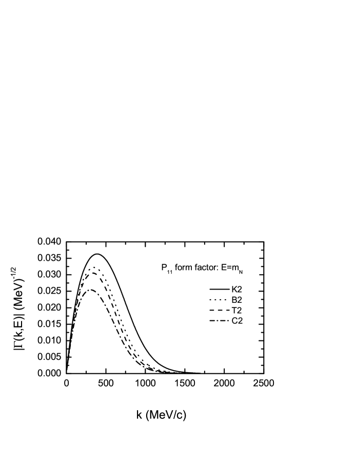
Figure 4: Our model predictions for the dressed $\pi NN$ vertex function $\Gamma(k,E)$, obtained with various reduction schemes and $n=2$ form factor.

The constructed four models can be considered approximately phase-shift equivalent. We therefore can examine how the resulting $\pi N$ off-shell dynamics depends on the chosen three-dimensional reduction. The $\pi N$ off-shell amplitudes are needed to study nuclear dynamics involving pions. To be specific, let us first discuss how the constructed models can be used to investigate the near threshold pion production from nucleon-nucleon collisions. The most important leading mechanism of this reaction is that a pion is emitted by one of the nucleons and then scattered from the second nucleon. The matrix element of this rescattering mechanism can be predicted by using the dressed $\pi NN$ form factor and the half-off-shell t-matrix. The predicted $\pi NN$ form factors for the near threshold kinematics, $E=m_{N}$, are compared in Fig. 4. In Fig. 5, we compare the half-off-shell t-matrix elements in the most relevant $S_{11}$ and $S_{31}$ channels at at pion lab. energy $1\,MeV$ above threshold. We see that there are rather significant differences between the considered reduction schemes at $k\geq 500$ MeV/c which is close to the momentum of the exchanged pion at the production threshold. Consequently, a study of near threshold pion production from NN collisions could distinguish the considered four different reduction schemes.

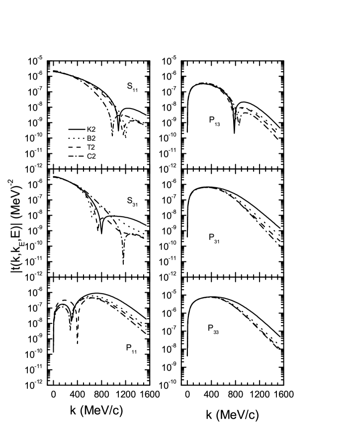
Figure 7: Same as Fig. 2 but at $E=1232\,MeV$ and for all S- and P-waves.

We next discuss the reactions at the $\Delta$ excitation region. In Figs. 6 and 7, we show the predicted dressed $\pi N\rightarrow\Delta$ form factor $\Gamma_{\pi N\Delta}$, defined analogously to $\Gamma_{\pi NN}$ of Eq. (40), and the half-off-shell t-matrix at the $\Delta$ resonance energy. These quantities are the input to the investigations of the $\Delta$ excitation in pion photoproduction [6, 8, 9]. The results shown in Figs. 6 and 7 suggest that the considered reduction schemes can also be distinguished by investigating the pion photoproduction reactions. This however requires a consistent derivation of the photoproduction formulation for each reduction scheme, and is beyond the scope of this work.

The differences shown in Figs. 6 and 7 can also have important consequences in determining pion-nucleus reactions in the $\Delta$ region. For instance, the constructed four models will give rather different predictions of pion double-charge reactions which are dominated by two sequential off-shell $\pi N$ single-charge exchange scattering. They can also be distinguished by investigating pion absorption which is induced by the dressed $\pi N\rightarrow\Delta$ vertex, Fig. 6, followed by a $N\Delta\rightarrow NN$ transition.

In summary, we have shown that the $\pi N$ scattering data up to 400 MeV can be equally well described by four reduction schemes of Bethe-Salpeter equation. The resulting meson-exchange models yield rather different off-shell dynamics. With the high quality data obtained in recent years, they can be best distinguished by investigating pion productions from NN collisions and pion photoproductions. Their differences in describing pion-nucleus reactions are also expected to be significant. Our effort in these directions will be published elsewhere.

Acknowledgment

We thank Drs. B. Pearce and C. Schütz for useful communications concerning their works. C.T.H. also wishes to thank Mr. Guan-yeu Chen for checking part of the program. This work is supported in part by the National Science Council of ROC under grant No. NSC82-0208-M002-17 and the U.S. Department of Energy, Nuclear Physics Division, under contract No.W-31-109-ENG-38, and also in part by the U.S.-Taiwan National Science Council Cooperative Science Program grant No. INT-9021617.

	BbS	Kady	Thomp	CJ
$\alpha(s,s^{\prime})$	$\eta_{N}(s^{\prime})\sqrt{\frac{s^{\prime}}{s}}$	$\eta_{N}(s^{\prime})\sqrt{\frac{s^{\prime}}{s}}$	$\eta_{N}(s)$	$\eta_{N}(s)$
$f(s,s^{\prime})$	1	$\frac{\sqrt{s}+\sqrt{s^{\prime}}}{2\sqrt{s^{\prime}}}$	$\frac{\sqrt{s}+\sqrt{s^{\prime}}}{2\sqrt{s}}$	$\frac{4\sqrt{ss^{\prime}}\varepsilon_{N}(s^{\prime})\varepsilon_{\pi}(s^{\prime})}{ss^{\prime}-(m_{N}^{2}-m_{\pi}^{2})^{2}}$

Table 1: The functions $\alpha(s,s^{\prime})$ and $f(s,s^{\prime})$ of Eq. (15), chosen for the four considered reduction schemes, i.e., Blankenbecler and Sugar ($BbS$) [20], Kadyshevsky ($Kady$) [21], Thompson ($Thomp$) [22], and Cooper and Jennings ($CJ$) [23].

Parameter	C2	B2	T2	K2
$m_{N}$	939	939	939	939
$m_{N}^{(0)}$	1090	1072	1071	1116
$m_{\pi}$	137	137	137	137
$m_{\Delta}$	1232	1232	1232	1232.
$m_{\Delta}^{(0)}$	1415	1412	1410	1461
$m_{\rho}$	770	770	770	770
$m_{\sigma}$	654	662	654	654.
$g_{\pi NN}^{2}/4\pi$	14.3	14.3	14.3	14.3
$g_{\pi NN}^{(0)^{2}}/4\pi$	3.82	6.28	5.49	6.08
$g_{\sigma NN}g_{\sigma\pi\pi}^{(s)}/4\pi$	-0.49	-0.37	-0.50	-0.39
$g_{\sigma NN}g_{\sigma\pi\pi}^{(v)}/4\pi$	33.20	-1.53	-1.40	-1.40
$g_{\rho NN}g_{\rho\pi\pi}/4\pi$	2.54	2.87	2.87	2.90
$\delta$	1.02	1.05	1.06	1.10
$g_{\pi N\Delta}^{2}/4\pi$	0.41	0.31	0.29	0.34
$g_{\pi N\Delta}^{(0)^{2}}/4\pi$	0.14	0.17	0.17	0.18
$Z$	-0.14	-0.036	-0.075	-0.029
$\kappa_{V}^{\rho}$	1.00	1.00	1.19	1.55
$\Lambda_{N}$	1227	1383	1321	1239
$\Lambda_{\sigma}$	417	704	681	648
$\Lambda_{\rho}$	1521	1700	1637	1548
$\Lambda_{\Delta}$	1026	1555	1542	1429
$\Lambda_{\pi}$	674	690	666	859

Table 2: The parameters of the constructed meson-exchange models, defined by Eqs. (29)-(36), are compared. The form factor Eq. (46) with $n=2$ is used. The models are constructed by using the three dimensional reduction schemes of Cooper and Jennings (C2), Blankenbecler and Sugar (B2), Thompson (T2), and Kadyshevsky (K2).

Parameter	T10	T2	K10	K2
$m_{N}$	939	939	939	939
$m_{N}^{(0)}$	1065	1071	1073	1116
$m_{\pi}$	137	137	137	137
$m_{\Delta}$	1232	1232	1232	1232
$m_{\Delta}^{(0)}$	1407	1410	1420	1461
$m_{\rho}$	770	770	770	770
$m_{\sigma}$	654	654	654	654
$g_{\pi NN}^{2}/4\pi$	14.3	14.3	14.3	14.3
$g_{\pi NN}^{(0)^{2}}/4\pi$	5.77	5.49	6.82	6.08
$g_{\sigma NN}g_{\sigma\pi\pi}^{(s)}/4\pi$	-0.49	-0.50	-0.39	-0.39
$g_{\sigma NN}g_{\sigma\pi\pi}^{(v)}/4\pi$	-1.52	-1.40	-1.43	-1.40
$g_{\rho NN}g_{\rho\pi\pi}/4\pi$	3.05	2.87	2.68	2.90
$\delta$	0.65	1.06	1.26	1.10
$g_{\pi N\Delta}^{2}/4\pi$	0.29	0.29	0.33	0.34
$g_{\pi N\Delta}^{(0)^{2}}/4\pi$	0.17	0.17	0.18	0.18
$Z$	-0.13	-0.075	-0.065	-0.029
$\kappa_{V}^{\rho}$	1.45	1.19	1.41	1.55
$\Lambda_{N}$	1300	1321	1373	1239
$\Lambda_{\sigma}$	653	681	400	648
$\Lambda_{\rho}$	1431	1637	2272	1548
$\Lambda_{\Delta}$	1522	1542	1507	1429
$\Lambda_{\pi}$	682	666	767	859

Table 3: The parameters of the constructed meson-exchange models, defined by Eqs. (29)-(36), are compared. The models are constructed by using the three dimensional reduction schemes of Thompson (T2,T10) and Kadyshevsky (K2,K10). T2 (T10) and K2 (K10) are models with n=2 (n=10) in defining the form factor of Eq. (46).

Figure 1: The driving terms of our model. (a) direct Born term, (b) u-channel nucleon exchange, (c) t-channel $\sigma$ exchange, (d) t-channel $\rho$ exchange, (e) s-channel $\Delta$ excitation, and (f) u-channel $\Delta$ exchange.

Figure 2: Our model predictions for $\pi N$ phase shifts in S- and P-waves obtained within Kadyshevsky reduction scheme and with the use of a $n=2$ form factor of Eq. (46). The data (solid triangles) are from [26].

Figure 3: Our model predictions for $P_{11}$ phase shifts obtained within Kadyshevsky (K2), Blankenbecler-Sugar (B2), Thompson (T2), and Cooper-Jennings (C2) reduction schemes, all with $n=2$ form factor. Data (solid triangles) are from Ref. [26].

Figure 5: Our model predictions for the half-off-shell $t-$matrix elements in $S_{11}$ and $S_{31}$ channels at pion lab. energy $1\,MeV$ above threshold, obtained with four different reduction schemes and $n=2$ form factor.

Figure 6: Our model predictions for the dressed $\pi N\Delta$ vertex $\Gamma_{\pi N\Delta}$ at $E=1232MeV$, obtained with various reduction schemes and $n=2$ form factor.

References

- [1] D. Ashery and J.P. Schiffer, Annu. Rev. Nucl. Part. Sci. 36, 207 (1986).
- [2] H.J. Weyer, Phys. Rep. 195, 295 (1990).
- [3] H. Kamada, M.P. Locher, T.-S. H. Lee, J. Golak, V.E. Markushin, W. Gloeckle and H. Witala, Phys. Rev. C 55, 2563 (1997).
- [4] T.-S. H. Lee and D.O. Riska, Phys. Rev. Lett. 70, 2237 (1993); C.J. Horowitz, H.O. Meyer, and D.K. Griegel, Phys. Rev. C 49, 1337 (1994); E. Hernandez and E. Oset, Phys. Lett. 350B, 158 (1995); C. Hanhart, J. Haidenbauer, A. Reuber, C. Schutz, and J. Speth, Phys. Lett. 358, 21 (1995).
- [5] B.-Y. Park, F. Myhrer, T. Meissner, J.R. Morones, and K. Kubodera, Phys. Rev. C 53, 1519 (1996); T.D. Cohen, J.L. Friar, G.A. Miller, and U. van Klock, Phys. Rev. C 53, 2661 (1996); T. Sato, T.-S. H. Lee, F. Myhrer, and K. Kubodera, Phys. Rev. C 56, 1246 (1997).
- [6] S.N. Yang, J. Phys. G11, L205 (1985); Phys. Rev. C 40, 1810 (1989).
- [7] C.C. Lee, S.N. Yang, and T.-S.H. Lee, J. Phys. G17, L131 (1991); S.N. Yang, Chin. J. Phys. 29, 485 (1991).
- [8] S. Nozawa, B. Blankleider and T.-S.H. Lee, Nucl. Phys. A513, 459 (1990).
- [9] T. Sato and T.-S. H. Lee, Phys. Rev. C 54, 2660 (1996).
- [10] M. Lacombe et al., Phys. Rev. C 21, 861 (1980).
- [11] R. Machleidt, K. Holinde, and Ch. Elster, Phys. Rep. 149, 1 (1987).
- [12] B.C. Pearce and B. Jennings, Nucl. Phys. A528, 655 (1991).
- [13] F. Gross and Y. Surya, Phys. Rev. C 47, 703 (1993).
- [14] C.T. Hung, Ph.D Thesis, National Taiwan University, 1994.
- [15] C.T. Hung, S.N. Yang and T.-S.H. Lee, J. Phys. G20, 1531 (1994).
- [16] C. Schütze, J.W. Durso, K. Holinde and J. Speth, Phys. Rev. C 49, 2671 (1994).
- [17] A. Klein and T.-S. H. Lee, Phys. Rev. D 10, 4308 (1974).
- [18] R.M. Woloshyn and A.D. Jackson, Nucl. Phys. B64, 269 (1974).
- [19] C. Itzykson and J.B. Zuber, Quantum Field Theory, McGraw-Hill, New York, 1980, Chapter 10.
- [20] R. Blankenbecler and R. Sugar, Phys. Rev. 142, 1051 (1966).
- [21] V.G. Kadyshevsky, Nucl. Phys. B6, 125 (1968).
- [22] R. H. Thompson, Phys. Rev. D 1, 110 (1970).
- [23] M. Cooper and B. Jennings, Nucl. Phys. A500, 553 (1989).
- [24] J. D. Bjorken and S. D. Drell, Relativistic Quantum Mechanics, McGraw-Hill, New York, 1964.
- [25] S. Morioka and I.R. Afnan, Phys. Rev. C 26, 1148 (1982); B.C. Pearce and I.R. Afnan, Phys. Rev. C 34, 991 (1986).
- [26] R. A. Arndt, I. I. Strakovsky and R. L. Workman, Phys. Rev. C 53, 430 (1996).