From the Bethe-Salpeter equation to non-relativistic approaches with effective two-body interactions

Abstract

It is known that binding energies calculated from the Bethe-Salpeter equation in ladder approximation can be reasonably well accounted for by an energy-dependent interaction, at least for the lowest states. It is also known that none of these approaches gives results close to what is obtained by using the same interaction in the so-called instantaneous approximation, which is often employed in non-relativistic calculations. However, a recently proposed effective interaction was shown to account for the main features of both the Bethe-Salpeter equation and the energy-dependent approach. In the present work, a detailed comparison of these different methods for calculating binding energies of a two-particle system is made. Some improvement, previously incorporated for the zero-mass boson case in the derivation of the effective interaction, is also employed for massive bosons. The constituent particles are taken to be distinguishable and spinless. Different masses of the exchanged boson (including a zero mass) as well as states with different angular momenta are considered and the contribution of the crossed two-boson exchange diagram is discussed. With this respect, the role played by the charge of the exchanged boson is emphasized. It is shown that the main difference between the Bethe-Salpeter results and the instantaneous approximation ones are not due to relativity as often conjectured.

, ,

1 Introduction

Understanding the discrepancies for binding energies obtained from different approaches, ranging from the ladder Bethe-Salpeter equation at one extreme [1] to a non-relativistic equation with a so-called instantaneous one-boson exchange interaction at the other extreme, has been and is still a subject which raises considerable interest and curiosity [2, 3, 4, 5, 6, 7, 8, 9, 10]. Although it is more founded theoretically, the Bethe-Salpeter equation in its simplest form (along with other approaches) is not doing as well as the Dirac or Klein-Gordon equation in reproducing the spectrum of atomic systems. These last equations assume a potential which is apparently consistent with an instantaneous propagation of the exchanged boson and their success has certainly contributed much in founding this approximation as a model for non-relativistic interactions.

It has been suggested that the problem was specific to QED together with the one-body limit [11] and irrelevant outside this case, when bosons are massive or the one-body limit does not apply. This is also supported by a number of works that motivated the instantaneous approximation from the Bethe-Salpeter equation. Although proofs are not transparent and rely on some approximations, allowing authors to have doubt [8], it is conjectured that including the contribution of crossed-boson exchange terms would resolve the problem [12, 13]. In this context, a few benchmark results emerge. It was clearly stated that the Bethe-Salpeter equation applied to the Wick-Cutkosky model [14] does not support the validity of the instantaneous approximation [2]. Instead, there is agreement with results from an energy-dependent interaction [3, 4]. The role of crossed boson exchange, as estimated using the Feynman-Schwinger representation (FSR) method [5], is also important in the case of massive bosons with equal-mass constituents.

Quite recently, two of the present authors, starting from a field-theory based approach, derived an effective interaction to be used in a non-relativistic framework [9]. It was found that this interaction, also obtained on a different basis in earlier works [15], involved a renormalization of the so-called instantaneous approximation. For small couplings, the renormalization factor is given by the probability of the system being in a two-body component, without accompanying bosons in flight. A close relation between wave functions issued from the field-theory (energy-dependent) scheme and the non-relativistic scheme (using an effective interaction) was found. It was suggested that the spectra obtained from the Bethe-Salpeter or other field-theory based approaches and that one resulting from the effective interaction could be quite similar for the lowest states. The role of crossed diagrams was also considered. In the case of a neutral, spinless boson it was found that their contribution largely cancels the renormalization of the instantaneous approximation interaction. While this result apparently provided support for the instantaneous approximation, its specific character was demonstrated by considering a model involving the exchange of “charged” bosons, which evidences a totally different pattern. Here, the contribution of crossed-boson exchange not only compensated the effect of the renormalization but provided even a lot more attraction in some cases. A first confirmation using the Bethe-Salpeter equation was obtained [10].

In this work, we consider a system of two scalar, distinguishable constituents that interact by the exchange of a scalar boson. This is the simplest case one can think of. It allows one to minimize complications with spin, like Z-type contributions for instance, which will obscure conclusions. We essentially want to compare binding energies with the main intent to establish a close relationship between the different approaches. This completes the work performed in ref. [9] for wave functions and extends it to the Bethe-Salpeter equation [10]. We will in particular study how this relationship is fulfilled when going from the ladder approximation to a more complete case involving crossed-boson exchange contributions. Regarding the latter, we will have in mind as benchmarks the results of Nieuwenhuis and Tjon [5] as well as those obtained in the so-called instantaneous one-boson exchange approximation. Our study will concentrate on systems with a rather small binding energy, of the order of what is reasonably accessible for a non-relativistic approach. An important issue is to determine which physics is behind some equation, with the idea that information obtained from the Bethe-Salpeter equation and a non-relativistic approach, the one more founded theoretically, the other closer to a physical interpretation, can complement each other. Quite generally, our aim is to derive effective interactions in a given scheme. This motivation has some similarity with the one underlying the work of Bhaduri and Brack who tried to reproduce the spectrum of the Dirac equation with an effective interaction in a non-relativistic approach [16]. The difference between this work and ours is in the dynamics: coupling of large and small components in one case, coupling of two-body components with components involving mesons in flight in the other. A renormalization of the instantaneous one-boson exchange interaction has been considered by Lepage [17]. This work has in common with the present one that it takes into account physics beyond some scale but it differs in the way how this physics is incorporated, parametrized in one case, theoretically motivated in the other.

The plan of the paper is as follows. In the second part, we remind essential theoretical ingredients relative to the different approaches that are referred to later on. These ones include the Bethe-Salpeter equation, an energy-dependent interaction resulting from time-ordered diagrams, an approach using an effective energy-independent interaction and finally an interaction in the instantaneous approximation. In the third section we present results obtained in the ladder approximation, incorporating higher-order box contributions in the effective approaches to allow for a consistent comparison with the Bethe-Salpeter results. Cases with massive as well as zero-mass bosons (Wick-Cutkosky model) are considered. The contribution due to crossed-boson exchange is examined and discussed in the fourth section. Two cases, corresponding to the exchange of neutral and charged bosons, are studied. The fifth section finally contains a general discussion and conclusions.

2 Descriptions of two-body systems: different approaches

In this section, we present the various approaches that will be used in the next sections to calculate binding energies of two-body systems. The first one is based on the Bethe-Salpeter equation which is well known for its manifestly relativistic covariant character. The field-theory foundation is more transparent in the second approach which is based on time-ordered diagrams and, therefore, gives an interaction that depends on the total energy of the system, $E$. This energy dependence is a reminiscent of the fact that the two-body system under consideration is coupled to components with bosons in flight. The third approach, which is derived from the previous one, is based on an effective interaction where the energy dependence has been eliminated. It differs in particular from the instantaneous one-boson exchange approximation, which is frequently employed in non-relativistic descriptions of two-body systems.

2.1 Bethe-Salpeter equation

The expression of the Bethe Salpeter equation for a system of scalar particles of mass $m$, interacting by the exchange of bosons of mass $\mu$, is well known. For definiteness, we nevertheless remind it here. It is given in momentum space by:

$$\left(m^{2}-(\frac{P}{2}+p)^{2}\right)\,\left(m^{2}-(\frac{P}{2}-p)^{2}\right)\;\Phi(p,P)=\hskip 56.9055pt$$

$$i\int\frac{d^{4}p^{\prime}}{(2\pi)^{4}}\,K(p,p^{\prime},P)\,\Phi(p^{\prime},P).$$ (1)

In this equation, $P$, $p$ and $p^{\prime}$ respectively denote the total momentum of the system and half of the relative momenta.

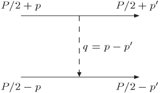
Figure 1: Graphical representation of the single-boson exchange contribution to the two-body interaction.

$K(p,p^{\prime},P)$ represents the interaction kernel. To lowest order it contains a well determined contribution due to one-boson exchange (see Fig. 1 for a graphical representation), its expression being given by:

$$K^{(1)}=-\frac{\tilde{g}^{2}\;O_{1}\,O_{2}}{\mu^{2}-t}\equiv-\frac{\tilde{g}^{2}\;O_{1}\,O_{2}}{\mu^{2}-(p-p^{\prime})^{2}-i\epsilon}.$$ (2)

Restricting the full kernel to this lowest order term, one obtains the ladder approximation of the Bethe-Salpeter equation, which has been extensively used in the literature. The coupling, $\tilde{g}^{2}$ in Eq. (2), has the dimension of a mass squared. The quantity $\frac{\tilde{g}^{2}}{4m^{2}}$ is directly comparable to the coupling constant $g^{2}$ which will be used in the following, to the coupling constant $g^{2}_{MNN}$, frequently used in hadronic physics, or to the quantity $4\pi\,\alpha$, where $\alpha$ is the usual QED coupling constant. Anticipating the following, we introduced the operators $O_{1}\,O_{2}$ in Eq. (2), that may be equal to $1_{1}\,1_{2}$ or $\vec{\tau}_{1}\cdot\vec{\tau}_{2}$ in the present work. The first case corresponds to the exchange of a neutral boson and the factor may be simply omitted. The second case corresponds to the exchange of bosons carrying some kind of isospin, equal to 1, while the constituents would have isospin $\frac{1}{2}$. The complete interaction kernel employed in Eq. (1) also contains multi-boson exchange contributions that Eq. (2) cannot account for, namely of the non-ladder type. As the simplest example of such contributions, we shall consider in Sect. 4 the crossed two-boson exchange. The numerical method we used to solve Eq. (1) and a detailed discussion was given in ref. [10].

2.2 Energy-dependent interaction from field-theory based one-boson exchange

The single-boson exchange contribution we want to consider is represented by the time-ordered diagrams of Fig. 2 .

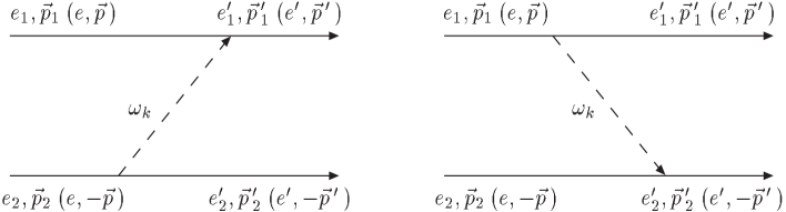
Figure 2: Time-ordered single-boson exchange contributions to the two-body interaction with indication of the kinematics in an arbitrary frame and in the center of mass (between parentheses).

The corresponding interaction is easily obtained from second-order perturbation theory:

$$V^{(1)}_{E}(,\vec{p}_{2},\vec{p}\,^{\prime}_{1},\vec{p}\,^{\prime}_{2})=\hskip 227.62204pt$$

$$\frac{g^{2}\;O_{1}\,O_{2}\,}{2\,\omega_{k}}\,\sqrt{\frac{m^{2}}{e_{1}e_{2}}}\,\left(\frac{1}{E-\omega_{k}-e_{1}-e^{\prime}_{2}}+\frac{1}{E-\omega_{k}-e_{2}-e^{\prime}_{1}}\right)\,\sqrt{\frac{m^{2}}{e^{\prime}_{1}e^{\prime}_{2}}},$$ (3)

with $\omega_{k}=\sqrt{\mu^{2}+(\vec{p}_{1}-\vec{p}\,^{\prime}_{1})^{\,2}},\;e_{i}=\sqrt{m^{2}+\vec{p_{i}}^{\,2}}$ and $e_{i}^{\prime}=\sqrt{m^{2}+\vec{p_{i}}^{\prime\,2}}.$ When the energy is conserved, this equation allows one to recover the standard Feynman propagator. In the center of mass, the two terms representing the contributions of the diagrams displayed in Fig. 2 are equal. Equation (3) then simplifies and reads:

$$V^{(1)}_{E}(\vec{p},\vec{p}\,^{\prime})=\frac{g^{2}\;O_{1}\,O_{2}\,}{\omega_{k}}\,\frac{m}{e}\,\left(\frac{1}{E-\omega_{k}-e-e^{\prime}}\right)\,\frac{m}{e^{\prime}},$$ (4)

with $\omega_{k}=\sqrt{\mu^{2}+\vec{k}^{\,2}},\;\vec{k}=\vec{p}-\vec{p}\,^{\prime},\;e=\sqrt{m^{2}+\vec{p}^{\,2}}$ and $e^{\prime}=\sqrt{m^{2}+\vec{p}\,^{\prime\,2}},\;$ where $\vec{p}$ and $\vec{p}\,^{\prime}$ represent the relative 3-momenta of the constituent particles. The two normalization factors, $\frac{m}{e}$ and $\frac{m}{e^{\prime}}$ in Eq. (4), are appropriate for the case where the total free energy of the constituent particles has the semi-relativistic expression, $e=\sqrt{m^{2}+\vec{p}^{\,2}}$, the corresponding equation to be fulfilled being of the Klein type [18]:

$$(2\,e-E)\,\psi(\vec{p}\,)=-\int\frac{d\vec{p}\,^{\prime}}{(2\pi)^{3}}\;\left(V^{(1)}_{E}(\vec{p},\vec{p}\,^{\prime})+\dots\right)\,\psi(\vec{p}\,^{\prime}).$$ (5)

The dots represent multi-boson exchange terms, some of which will be explicitly considered in the following. An important feature of the interaction (4) is its dependence on the total energy of the system, $E$, which prevents one from using it in a Schrödinger equation without some caution. This energy dependence has the same origin as the one in the full Bonn model of the nucleon-nucleon interaction [19]. It is reminded that the above equation may be obtained from the Bethe-Salpeter equation, Eq. (1), by putting:

$$\left(m^{2}-(\frac{P}{2}+p)^{2}\right)\,\left(m^{2}-(\frac{P}{2}-p)^{2}\right)\;\Phi(p,P)\hskip 113.81102pt$$

$$\simeq\left(2\,e\right)^{2}\;\left(e-\frac{E}{2}-p_{0}\right)\;\left(e-\frac{E}{2}+p_{0}\right)\;\Phi(p,P)\hskip 28.45274pt$$

$$\equiv\frac{2\,e}{E}\;(2e-E)\,\psi(\vec{p}\,),\hskip 28.45274pt$$ (6)

consistently neglecting the dependence on $p_{0}$ (but not $p^{\prime}_{0}$!) in the kernel as well as corrections of order $\frac{E-2e}{2\,E}$ (we assume that the mass of the exchanged boson, $\mu$, is smaller than the constituent mass, $m$). In accordance with the center of mass validity of Eq. (4), $P_{0}$ has been replaced by $E$. It is also reminded that an equation like Eq. (5) (or similar ones used below) can always be cast into the form of a 4-dimensional, but non-covariant equation, as it can be checked from the following:

$$(2e-E)\;\psi(\vec{p}\,)=i\int\frac{d^{4}p\,^{\prime}}{(2\pi)^{4}}\;\,\frac{\left(V^{(1)}_{E}(\vec{p},\vec{p}\,^{\prime})+\dots\right)\;\;(2e^{\prime}-E)\,\psi(\vec{p}\,^{\prime})}{\left(e^{\prime}-\frac{E}{2}-p^{\prime}_{0}+i\epsilon\right)\;\left(e^{\prime}-\frac{E}{2}+p^{\prime}_{0}+i\epsilon\right)}.$$ (7)

A non-relativistic, but still energy-dependent form of Eq. (5) may be used:

$$\left(\frac{p^{2}}{m}-(E-2m)\right)\,\psi(\vec{p}\,)=-\int\frac{d\vec{p}\,^{\prime}}{(2\pi)^{3}}\;\left(V^{(1)}_{E}(\vec{p},\vec{p}\,^{\prime})+\dots\right)\;\psi(\vec{p}\,^{\prime}),$$ (8)

where the normalization factors $\frac{m}{e}$ appearing in $V^{(1)}_{E}$ should be consistently neglected. This last equation represents an intermediate step in our effort to derive an effective non-relativistic interaction in the next subsection.

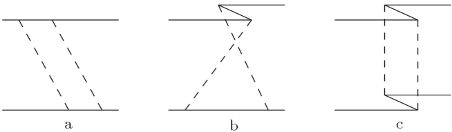
Figure 3: Box type two-boson exchange contributions to the two-body interaction in time-ordered perturbation theory.

In order to make a meaningful comparison with the ladder Bethe-Salpeter approach, box-type multi-boson exchange contributions to the interaction $V_{E}$ should be considered. Some of them are shown in Fig. 3. The most important one corresponds to diagram a) in this figure. Its contribution is of order $\left(\frac{1}{m}\right)^{0}$ and has the same magnitude as the off-shell effects due to the presence of the term $E-e-e^{\prime}$ in the denominator of Eq. (4) (see also ref. [9]). Its expression is given by:

$$V^{(2a)}(\vec{p\,},\vec{p}\,^{\prime})=-\frac{g^{4}}{2}\int\frac{d\vec{q}}{(2\pi)^{3}}\;\frac{m}{e}\frac{(O_{1}\,O_{2})\,(O_{1}\,O_{2})}{\omega\,\omega^{\prime}}\frac{m}{e^{\prime}}\left(\frac{m}{e_{q}}\right)^{2}\hskip 56.9055pt$$

$$\times\frac{1}{\left(\omega+e+e_{q}-E\right)}\frac{1}{\left(\omega^{\prime}+e^{\prime}+e_{q}-E\right)}\frac{1}{\left(\omega+\omega^{\prime}+e+e^{\prime}-E\right)},$$ (9)

with $\omega=\sqrt{\mu^{2}+(\vec{p}-\vec{q}\,)^{2}}$, $\omega^{\prime}=\sqrt{\mu^{2}+(\vec{p}\,^{\prime}-\vec{q}\,)^{2}}$ and $e_{q}=\sqrt{m^{2}+\vec{q}\,^{\,2}}$. The quantity $\vec{q}$ represents the momentum of the constituent particle in the intermediate state and the operators $O_{i}$ are put between parentheses to remind that they do not necessarily commute. As we do not pay much attention to contributions of order $g^{6}$, one could be tempted to drop terms like $E-e-e^{\prime}$ in the denominator of Eq. (9), which are of the same order. Doing this also has the advantage that the integral of Eq. (9) can be worked out analytically (see Appendix A). We shall nevertheless retain the full expression of Eq. (9) in our calculations, in order to deal consistently with the energy dependence of the box diagram. Numerically, the effect of the latter one turned out to be substantial. On the other hand, contributions of Z-diagrams like Fig. 3 b,c have a typical relativistic character and are of order $\left(\frac{1}{m}\right)^{1}$ and $\left(\frac{1}{m}\right)^{3}$, respectively.

The expression of the interaction given by Eq. (4) is much simpler than the one used in ref. [3], which was however derived on a different basis. The latter one most probably incorporates higher order corrections like those of Fig. 3 b,c, and, furthermore, should be used with a different equation.

2.3 Energy-independent approach and effective interaction

In order to get an energy-independent interaction from the general interaction kernel given by Eq. (4), the energy dependence of the latter one was approximated in ref. [9] by a linear term (see ref. [20] for examples in relation with the present work):

$$\frac{1}{E-2m-\omega_{k}-\frac{\vec{p}^{\,2}}{2m}-\frac{\vec{p}\,^{\prime\,2}}{2m}}=-\frac{1}{\omega_{k}}-\frac{E-2m-\frac{\vec{p}^{\,2}}{2m}-\frac{\vec{p}\,^{\prime\,2}}{2m}}{\omega^{2}_{k}}+\cdots,$$ (10)

where we replaced, as we shall do from now on, the relativistic expressions for the kinetic energies by their non-relativistic counterparts. The second term on the right hand side of Eq. (10), after insertion in Eqs. (5) or (8), was then removed by a transformation which is formally similar to the one introduced by Perey and Saxon [21] in order to change a linear energy-dependent term of an optical potential into a dependence on the squared momentum and vice versa. The inverse transformation is used for solving an equation with a squared momentum-dependent term when employing the Numerov algorithm. In both cases, it has no definite physical ground beyond its mathematical character. The transformation which was performed here is more in the spirit of the Foldy-Wouthuysen one (see ref. [9] for details). It implicitly corresponds to introducing effective degrees of freedom with the drawback that the interaction generally acquires a non-local character. An expansion similar to that given in Eq. (10) was used by Lahiff and Afnan [22], so that some of our results obtained with the full energy dependence of the interaction kernel have a relationship to theirs. However, these authors have not considered the possibility of removing the energy dependence by the transformation mentioned above. The resulting energy-independent interaction is the main object of studies in the present work.

Since the expansion parameter in Eq. (10) is roughly equivalent to the interaction strength, this equation makes sense as long as the coupling is not too large. In the present work, we will improve upon this approximation, extending to massive bosons what was done in ref. [9] for the zero-mass case. In the latter one, the Coulomb-like potential kept its analytical form, only the coupling constant was renormalized by a factor that was determined by solving a self-consistency equation. The zero-mass case will be reminded in Sect. 3.2 below, together with further developments.

Starting from the formal expression of the interaction in configuration space:

$$V_{E}(r)=g^{2}\;O_{1}\,O_{2}\;\frac{1}{2\pi^{2}}\int\frac{dkk^{2}j_{0}(kr)}{\omega_{k}\left(E-2m-\omega_{k}-\frac{\vec{p}^{\,2}}{2m}-\frac{\vec{p}\,^{\prime\,2}}{2m}\right)},$$ (11)

we assume that the quantity $E-2m-\frac{\vec{p}^{\,2}}{2m}-\frac{\vec{p}\,^{\prime\,2}}{2m}$ in the denominator under the integral can be approximated by the effective potential we want to determine. This procedure is often used in other domains of physics where it underlies for instance the Thomas-Fermi-, WKB-, or eikonal approximations [23, 24], and it immediately provides a self-consistency equation:

$$V^{nr}_{eff,sc}(r)=-g^{2}\;O_{1}\,O_{2}\;\frac{1}{2\pi^{2}}\int\frac{dkk^{2}j_{0}(kr)}{\omega_{k}\left(\omega_{k}-V^{nr}_{eff,sc}(r)\right)}.$$ (12)

By neglecting the effective interaction under the integral, one recovers the standard expression of the instantaneous one-boson exchange potential:

$$V_{0}(r)=-g^{2}\,O_{1}\,O_{2}\;\frac{e^{-\mu r}}{4\pi r}.$$ (13)

One can go a step further and make an expansion of the r.h.s. of Eq. (12) up to first order in the effective potential:

$$V^{nr}_{eff}(r)=V_{0}(r)-V^{nr}_{eff}(r)\;V_{1}(r),$$ (14)

where

$$V_{1}(r)=g^{2}\;O_{1}\,O_{2}\;\frac{1}{2\pi^{2}}\int\frac{dkk^{2}j_{0}(kr)}{(\omega_{k})^{3}}=\frac{g^{2}\;O_{1}\,O_{2}}{2\pi^{2}}\;K_{0}(\mu r).$$ (15)

By rearranging terms in Eq. (14), one recovers the expression of the effective interaction given in ref. [9]:

$$V^{nr}_{eff}(r)=\frac{V_{0}(r)+...}{\left(1+V_{1}(r)+...\right)},$$ (16)

where the dots may account for two, three, … boson exchange. This expression has a simple interpretation in the limit of small couplings. It corresponds to the instantaneous approximation potential renormalized by the probability that the system is in a two-body component. Notice that the self-consistent potential of Eq. (12) can be put in a form analogous to Eq. (16), with a generalized renormalization factor:

$$V^{nr}_{eff,sc}(r)=\frac{V_{0}(r)+...}{1+\frac{g^{2}\;O_{1}\,O_{2}}{2\pi^{2}}\int\frac{dkk^{2}j_{0}(kr)}{\omega_{k}^{2}\left(\omega_{k}-V^{nr}_{eff,sc}(r)\right)}+...}.$$ (17)

While making the above developments, we assumed that the operator $p^{2}$ could be treated as a number. To go beyond this approximation, an expansion of the denominator in Eq. (11) should be performed in the vicinity of

$$E-2m-\frac{\vec{p}^{\,2}}{2m}-\frac{\vec{p}\,^{\prime\,2}}{2m}\simeq V^{nr}_{eff,sc}(r).$$ (18)

This approximate equality is valid provided it is applied to a solution of a Schrödinger equation. One thus gets up to first order in the expansion:

$$V_{E}(r)=V^{nr}_{eff,sc}(r)+\frac{1}{2}\left\{\left(\frac{\vec{p}^{\,2}}{m}+V^{nr}_{eff,sc}(r)+2m-E\right),V_{1,sc}(r)\right\},$$ (19)

where

$$V_{1,sc}(r)=g^{2}\;O_{1}\,O_{2}\;\frac{1}{2\pi^{2}}\int\frac{dkk^{2}j_{0}(kr)}{\omega_{k}\left(\omega_{k}-V^{nr}_{eff,sc}(r)\right)^{2}}$$ (20)

generalizes the result given by Eq. (15). The expression of Eq. (19) can now be inserted in the equation that corresponds to Eq. (8) in configuration space. One thus gets the following equation with an energy-dependent interaction:

$$\Bigg{(}V^{nr}_{eff,sc}(r)(1+V_{1,sc}(r))+\frac{1}{2}\left\{\frac{\vec{p}^{\,2}}{m},\Big{(}1+V_{1,sc}(r)\Big{)}\right\}\hskip 85.35826pt$$

$$-(E-2m)\Big{(}1+V_{1,sc}(r)\Big{)}\Bigg{)}\psi(r)=0.$$ (21)

The equation relative to the energy-independent scheme is obtained by multiplying Eq. (21) from the left by $\Big{(}1+V_{1,sc}(r)\Big{)}^{-1/2}$ and making the substitution:

$$\psi(r)=\Big{(}1+V_{1,sc}(r)\Big{)}^{-1/2}\,\phi(r).$$ (22)

One thus gets a usual non-relativistic Schrödinger equation:

$$\left(V_{eff}(r)+\frac{\vec{p}^{\,2}}{m}-(E-2m)\right)\phi(r)=0,$$ (23)

with an effective potential

$$V_{eff}(r)=V^{nr}_{eff,sc}(r)-\frac{1}{4m}\frac{\left(\vec{\nabla}V_{1,sc}(r)\right)^{2}}{\Big{(}1+V_{1,sc}(r)\Big{)}^{2}}.$$ (24)

The (presumably) dominant first term, of order $\left(\frac{1}{m}\right)^{0}$, has a typical non-relativistic character. It can be checked that its contribution to order $g^{4}$ (i.e. including the box diagram, Fig. 3 a) is identical to the one obtained by substracting from the Feynman two-boson exchange diagram that part resulting from iterating the one-boson exchange. This represents another way of calculating the contributions to energy-independent potentials with the range of two-boson exchange [25, 26]. However, the present approach allows one to take into account higher order corrections that are relevant when $V_{1,sc}(r)$ becomes large. The second term in Eq. (24) is required for consistency with Eq. (21) and, most importantly, it represents the first correction to the approximation given by Eq. (18) at the denominator of Eq. (11). Being of a higher order in $\frac{1}{m}$, it will be neglected in most calculations using the effective interaction. This is consistent with neglecting other relativistic corrections of the same order, especially the normalization factors $\frac{m}{e}$ present in Eq. (4). These ones provide some non-locality that, most probably, could be accounted for in the above developments, but at the price of a tremendous numerical work. For the same reason, we will retain, for the numerical calculations presented below, the expression of the self-consistent, effective potential given by the solution of Eq. (12). When accounting for the higher-order terms in $\frac{1}{m}$, the derivation of the effective potential proceeds analogously, by incorporating the second term of Eq. (24) in the self-consistency equation.

The dressed (effective) character of the object described by $\phi(r)$, Eq. (23), is better seen by looking at the expression of the norm in the local approximation:

$$N=\int d\vec{r}\;\phi^{2}(r)=\int d\vec{r}\;\bigg{(}\frac{\phi^{2}(r)}{\Big{(}1+V_{1,sc}(r)\Big{)}}+\frac{\phi^{2}(r)\;V_{1,sc}(r)}{\Big{(}1+V_{1,sc}(r)\Big{)}}\bigg{)}=\hskip 28.45274pt$$

$$\int d\vec{r}\;\left(\psi^{2}(r)+\psi(r)\,V_{1,sc}(r)\,\psi(r)\right).$$ (25)

The quantity $\phi^{2}(r)$ describes a hybrid state that is a coherent superposition of two components, with weights respectively given by $\frac{1}{1+V_{1,sc}(r)}$ and $\frac{V_{1,sc}(r)}{1+V_{1,sc}(r)}$. The first one, which from Eq. (22) is seen to be described by $\psi(r)$, corresponds to the bare two-body component. The second one, which corresponds to a three-body component, has a more complicated structure. The relation in this case can be obtained from the expression of the component with one boson in flight:

$$|{\rm boson}+2\,{\rm constituents}\rangle=\frac{1}{E-\omega_{k}-e_{1}-e_{2}}\,H_{I}\,|2\,{\rm constituents}\rangle,$$ (26)

where $H_{I}$ is the boson-constituent interaction. Using this expression, it can be checked that the part corresponding to extra bosons in flight (discarding the boson cloud of the constituents) provides a contribution to the normalization given by $\int d\vec{r}\;\psi^{2}(r)(-\frac{\partial V_{E}(r)}{\partial E})$. The identification with the last term in Eq. (25) is achieved via the expression given by Eq. (19), or equivalently from an explicit calculation starting with Eq. (11), allowing one to directly obtain Eq. (20).

2.4 Instantaneous one-boson exchange approximation

It is noticed that the potential of Eq. (24) does not correspond to the so-called instantaneous approximation given by $V_{0}(r)$ in Eq. (13). This one, which is often used as a reference, underlies many models dealing with hadronic systems and, at first sight, the well known Coulomb potential. It can be partly justified as follows. Starting from the usual covariant expression for a boson propagator in configuration space,

$$\Delta(x_{1}-x_{2})=i\int\,\frac{d^{4}q}{(2\pi)^{4}}\,\frac{e^{iq\cdot(x_{1}-x_{2})}}{\mu^{2}+\vec{q}^{\,2}-q_{0}^{2}-i\epsilon},$$ (27)

and assuming that the energy transfer $q_{0}$ is small, one gets

$$\Delta_{B}(x_{1}-x_{2})\simeq i\,\delta(t_{1}-t_{2})\,\frac{e^{-\mu\,r}}{4\pi r},\;\;\;({\rm with}\;r=|\vec{r}_{1}-\vec{r}_{2}|).$$ (28)

The assumption that $q_{0}$ is small is valid for a Born amplitude in the non-relativistic domain. Beyond this approximation, $q_{0}$, which is an integration variable at the r.h.s. of Eq. (27), is not limited to small values. It may be large and, in particular, can give rise to singularities when $q_{0}=\pm\sqrt{\mu^{2}+\vec{q}^{\,2}}$. These poles are responsible for the renormalization of the so-called instantaneous potential, Eq. (13), leading to the effective potential of Eq. (24). Their contributions are omitted in the spectator approach [27] where they could allow one to symmetrize the role of the two constituent particles. This omission is generally justified by the fact that these extra contributions are cancelled by crossed-boson exchange diagrams, thus recovering an instantaneous-like single-boson exchange interaction. However, this only works for neutral, spinless bosons, which discards two important cases in hadronic physics: pions and gluons.

While the potentials of Eqs. (24) and (13) both have an instantaneous character, there is not necessarily a contradiction as they do not correspond to the same mathematical description. In one case, one works with asymptotic, bare particles that exchange bosons. In the other, one works with dressed particles that are eigenstates of the Hamiltonian, incorporating components with bosons in flight. The concept of an instantaneous propagation of the interaction is therefore partly scheme dependent. It will become clear from our results that the effects implicitly incorporated in the effective interaction account at least partially for the dynamics of the original relative time (or energy) variable, which has been integrated out (as for instance in Eq. (5)). The effects under discussion may therefore not be relativistic ones as sometimes advocated in the literature. Instead, they are quite similar to those appearing in the many-body problem. In the case of the nucleon-nucleus interaction for instance, they originate from the energy dependence of the optical potential due to the coupling to other channels, whose effects can be partly incorporated in mean-field approximations through a contribution to the effective mass [24]. The close relationship between the quasi-particle strength introduced in that work, $Z=(1-\frac{d}{dE}\Delta V(E))^{-1}$, and the quantity $(1+V_{1})^{-1}$ appearing in many equations of the present section, is evident.

The non-relativistic character of the effects we are looking at is further supported by the examination of the energy denominator obtained from time-ordered diagrams, which describes the evolution of the system from time $t_{1}$ to time $t_{2}$. This quantity contains the energy of the exchanged boson $\omega_{k}$ and, also, the difference of the total energy of the system and the energies of the constituents, $E-e-e^{\prime}$. The non-relativistic limit of this last factor can be taken but, appearing on the same footing as the $\omega_{k}$ term, it cannot be put to zero as the so-called instantaneous approximation would suppose. At best, it can be considered as a recoil correction of order $\frac{\mu}{m}$. This can be seen by expanding the energy denominator appearing in Eq. (4),

$$E-e-e^{\prime}-\omega_{k}=-\mu-\frac{(\vec{p}-\vec{p}\,^{\prime})^{2}}{2\mu}-\frac{\vec{p}^{\,2}}{2m}-\frac{\vec{p}\,^{\prime\,2}}{2m}+...$$ (29)

On the other hand, corrections which arise from the expansion of Eq. (4) up to terms of order $\frac{1}{\omega^{3}}$, are consistent with Galilean invariance in the standard non-relativistic approximation where $e_{p}$ is replaced by $m+\frac{p^{2}}{2m}$. This supposes that the contributions of both two terms in Eq. (3) are taken into account. It can indeed be shown that the complete numerator of the second term in the expansion given by Eq. (10) is then independent of the total momentum, as it follows from the equality

$$E_{c.m.}+\frac{(\vec{p_{1}}+\vec{p_{2}})^{\,2}}{4m}-\frac{\vec{p_{1}}^{\,2}}{4m}-\frac{\vec{p_{2}}^{\,2}}{4m}-\frac{\vec{p_{1}}\,^{\prime\,2}}{4m}-\frac{\vec{p_{2}}\,^{\prime\,2}}{4m}=E_{c.m.}-\frac{\vec{p}^{2}}{2m}-\frac{\vec{p}\,^{\prime\,2}}{2m},$$

where $E_{c.m.}$ is the energy in the center of mass (simply written $E$ elsewhere in the text). The corrections under discussion are therefore completely consistent with a non-relativistic approach.

Corrections of higher order in $\frac{1}{\omega}$ depend on the total momentum of the system. Contrary to the previous ones, they have a relativistic character, accounting in particular for the fact that two events that occur in a given order in one frame may occur in a different order in another one. This effect is also closely related to the occurence of two different terms in Eq. (3), which reduce to a single one in the center of mass system.

Being justified in the Born approximation, the one-boson exchange instantaneous approximation cannot correctly account for higher order (off-shell) effects. How large these ones are will be discussed in the next sections where binding energies are compared with corresponding ones of more complete approaches. The above statement also applies to the many quasi-potential approaches that have been considered in the literature [27, 28], often with the idea to provide some link to the Bethe-Salpeter equation. Frequently, they differ by the two-particle propagator while using an interaction similar to the so-called instantaneous approximation. Little attention has been given to a significant modification of the interaction, like the one provided by a renormalization as given by Eq. (24). This one, as will be seen below, is essential to reveal the close relationship with the Bethe-Salpeter equation. Notice that, in the domain of hadronic physics, this renormalization is accounted for correctly in different ways at the two-pion level in the Paris [26] and full Bonn [19] models of the NN interaction, but treated phenomenologically in most other ones.

Energy-dependent corrections beyond the instantaneous approximation, which we are interested in here, have different names, depending on the domain where they are employed: norm corrections in the case of mesonic exchange currents [29], dispersive effects in scattering processes involving composite systems [24] or retardation effects in two-body scattering [19]. It is remarked that retardation effects sometimes represent different kind of corrections, involving terms of the order $\left(\frac{\Delta E}{\omega}\right)^{2}$ [13], rather than the ones retained here, that involve terms of the order $\frac{\Delta E}{\omega}$. As already mentioned, the former ones are of the order $\left(\frac{1}{m}\right)^{2}$, and have a typical relativistic character.

2.5 Some notes on abnormal states

It is a common feature of all non-relativistic reduction formalisms of the Bethe-Salpeter equation, that the original relative time degree of freedom is somehow eliminated. One is thereby faced with the question whether an essential dynamical ingredient is lost in this step and if yes, how to recover it. The main motivation of this work came from the conviction that the dynamics involving the relative time can indeed be accounted for in a non-relativistic scheme. If this is the case, also excited states should be well described in an effective approach. This is why we shall put some emphasis on the simultaneous description of ground and excited states when we present our results in the next section.

If we claim that the dynamics of the time variable is well described in a non-relativistic approach, one may immediately ask about states, that are intrinsically connected to this fourth variable, that are the so-called abnormal states. Being excitations in the fourth dimension, it is difficult to imagine describing them in a three-dimensional formalism. It was noted however [7] that just this may be achieved by an energy-dependent potential. The existence of “extra” solutions (i.e. solutions that do not have an analogue when the energy dependence in the potential is neglected) to the Schrödinger equation was analytically demonstrated in ref. [30]. The authors considered the equivalent of our Eq. (8) for the zero-mass boson case ($\mu=0$). The key point was the observation, that the asymptotic behaviour of the potential in configuration space changes discontinuously at large distances if the energy dependence is kept. The potential then takes the asymptotic form

$$V_{E}(r)|_{Er\gg 1}\sim-\frac{2\alpha}{Er^{2}},$$ (30)

instead of the usual Coulomb potential $V_{E=0}(r)=-\frac{\alpha}{r}$. Thereby, a new class of solutions appears, characterized by a radial wave function with an infinity of zeroes. It was also noted, that these solutions exist only for large values of the coupling constant, which is just what happens in the relativistic analogue of this case, the Wick-Cutkosky model [14].

It seems possible therefore to account for abnormal states even in a three-dimensional formalism. Unfortunately, neither of the effective interaction potentials that we shall use, Eq. (12) and Eq. (16), even though they are supposed to account for a part of the energy dependence of the original potential that they were derived from, will be able to produce these supplementary states. The reason is, that they both have the same asymptotic behaviour for large distances in configuration space as the original Coulomb potential, so the argument of ref. [30] does not apply. This shows the nonperturbative nature of these states and the necessity to keep track of the full energy dependence of the original potential if one wants to account for them. However, from a calculational point of view, it seems to be difficult to identify these solutions numerically, since there is no obvious criterion to distinguish them from normal ones. For that reason and in order to render a comparison meaningful for all approaches considered here, we shall only investigate normal states in this work.

3 Results in ladder approximation

We present here binding energies calculated in ladder approximation using the different approaches described in the last section. Explicitly, these ones include:

• the Bethe-Salpeter (B.S.) equation, Eq. (1), together with an interaction kernel given by Eq. (2) (ladder approximation),

• a semi-relativistic equation, Eq. (5), with an energy-dependent interaction ($V_{E}$) given by Eq. (4),

• the standard non-relativistic Schrödinger equation, Eq. (23), together with an effective interaction ($V_{eff,sc}$) given by Eq. (12), which accounts for energy-dependent effects in a self-consistent calculation,

• the same equation, but with an effective interaction ($V_{eff}$) as given by Eq. (16), accounting for energy-dependent effects only at the lowest order,

• the same equation in the so-called instantaneous approximation (IA) with an interaction given by Eq. (13).

In Fig. 4, we plot the potential functions of the last three of these approaches in configuration space with the box contribution included for two values of the coupling constant and two values of the boson mass. It can be seen that the effective potentials are significantly smaller than the instantaneous approximation, especially at small distances, the effect being larger for $V_{eff}$ than for its self-consistent version, $V_{eff,sc}$.

      

      

Figure 4: Representation of non-relativistic potentials for two values of $\alpha$ and two values of $\mu$. $V_{0}$ is the instantaneous potential of Eq. (13), $V_{eff}$ is the effective potential of Eq. (16) and $V_{eff,sc}$ gives the self-consistent, effective potential of Eq. (12).

In the following, we give results for the above two different boson masses as well as different angular momenta. The aim is to show that binding energies are relatively close to each other for the four first approaches and significantly depart from those obtained in the instantaneous one-boson exchange approximation. In the second, third and fourth approaches, the results with and without the contribution of the box diagram (Fig. 3 a) are considered, so that a comparison with the Bethe-Salpeter approach is fully relevant at order $\left(\frac{1}{m}\right)^{0}$.

3.1 Finite-mass boson case

Table 1: Binding energies calculated in the ladder approximation for massive scalar bosons (in units of the constituent mass $m$). Results are presented here as a function of the coupling constant $\alpha$ for the ground state ($l=0$) and two boson masses ($\mu=0.15\,m$ and $\mu=0.5\,m$). Five cases have been considered: the Bethe-Salpeter equation (B.S., Eqs. (1, 2)), an energy-dependent model ($V_{E}$, Eqs. (4, 5)), an effective non-relativistic interaction ($V^{nr}_{eff,sc}$, Eqs. (23, 12)), a simplified version of this effective interaction ($V^{nr}_{eff}$, Eqs. (23, 16)) and, slightly apart, the so-called instantaneous approximation (IA^nr, Eqs. (23, 13)). In the second, third and fourth cases, the binding energies calculated without the contribution of the box diagram are given between parentheses. The superscript nr reminds that the calculations are performed with an interaction derived at the lowest order, $\left(\frac{1}{m}\right)^{0}$.

$\mu/m$	$\alpha$	${\rm B.S.}$	$V_{E}\;(-{\rm box})$	$V^{nr}_{eff,sc}\;(-{\rm box})$	$V^{nr}_{eff}\;(-{\rm box})$		${\rm IA}^{nr}$
	$0.50$	0.0059	0.0052 (0.0045)	0.0062 (0.0051)	0.0055 (0.0040)		0.013
	$0.75$	0.023	0.020 (0.017)	0.023 (0.020)	0.020 (0.014)		0.056
$.15$	$1.00$	0.047	0.039 (0.034)	0.048 (0.039)	0.038 (0.026)		0.129
	$1.25$	0.076	0.061 (0.052)	0.076 (0.063)	0.059 (0.037)		0.233
	$1.50$	0.109	0.084 (0.073)	0.108 (0.088)	0.081 (0.047)		0.367
	$1.50$	0.0125	0.0071 (0.0051)	0.0144 (0.0090)	0.0098 (0.0028)		0.093
	$1.75$	0.028	0.017 (0.013)	0.031 (0.021)	0.023 (0.008)		0.180
$.50$	$2.00$	0.049	0.030 (0.024)	0.053 (0.037)	0.038 (0.014)		0.296
	$2.25$	0.073	0.045 (0.036)	0.078 (0.056)	0.056 (0.022)		0.442
	$2.50$	0.100	0.061 (0.050)	0.106 (0.077)	0.077 (0.030)		0.619

Table 2: Same as Table 1 for excited states with $l=0^{*}$ and $l=1$. Bars indicate that there is either no bound state or that its binding energy, being too small, cannot be determined reliably.

$\mu/m$	$l$	$\alpha$	${\rm B.S.}$	$V_{E}\;(-{\rm box})$	$V^{nr}_{eff,sc}\;(-{\rm box})$	$V^{nr}_{eff}\;(-{\rm box})$		${\rm IA}^{nr}$
		$2.00$	0.005	0.003 (0.002)	0.006 (0.004)	0.003 ( —– )		0.054
		$2.25$	0.010	0.006 (0.004)	0.011 (0.007)	0.005 ( —– )		0.086
	$0^{*}$	$2.50$	0.015	0.009 (0.007)	0.016 (0.011)	0.009 (0.001)		0.124
		$2.75$	0.022	0.013 (0.010)	0.023 (0.015)	0.013 (0.002)		0.170
		$3.00$	0.029	0.018 (0.014)	0.030 (0.021)	0.018 (0.003)		0.223
$0.15$
		$2.00$	0.003	0.002 (0.001)	0.003 (0.001)	0.002 ( —– )		0.042
		$2.25$	0.009	0.006 (0.003)	0.009 (0.005)	0.006 (0.001)		0.073
	$1$	$2.50$	0.015	0.011 (0.007)	0.015 (0.009)	0.011 (0.003)		0.111
		$2.75$	0.022	0.016 (0.011)	0.022 (0.014)	0.016 (0.005)		0.156
		$3.00$	0.030	0.022 (0.016)	0.029 (0.020)	0.022 (0.007)		0.209
		$9$	0.022	( — ) ( —– )	0.031 (0.012)	0.017 ( —– )		1.787
		$10$	0.042	0.004 (0.001)	0.053 (0.024)	0.035 ( —– )		2.494
	$0^{*}$	$11$	0.067	0.012 (0.005)	0.079 (0.040)	0.057 ( —– )		3.324
		$12$	0.096	0.022 (0.011)	0.108 (0.058)	0.084 ( —– )		4.279
$0.5$
		$9$	0.012	( — ) ( —– )	0.014 ( —– )	( — ) ( —– )		1.627
		$10$	0.037	0.003 ( —– )	0.039 (0.008)	0.022 ( —– )		2.327
	$1$	$11$	0.067	0.015 (0.002)	0.067 (0.026)	0.046 ( —– )		3.150
		$12$	0.101	0.031 (0.012)	0.099 (0.046)	0.075 ( —– )		4.099

Calculations have been performed with boson masses $\mu=0.15\,m$ and $\mu=0.5\,m$, a choice that was made in earlier works [5, 6]. In the instantaneous approximation, these results are not independent. The ratio of the binding energy and the squared boson mass is a unique function of the ratio of the coupling constant and the boson mass:

$$\frac{m\,E_{be}}{\mu^{2}}=f\left(\frac{\alpha m}{\mu}\right).$$ (31)

For the coupling constant, $\alpha=\frac{g^{2}}{4\pi}$, we considered ranges appropriate for the states under consideration, in order to provide a significant insight on the variation of the binding energy with the strength of the interaction. Some of the binding energies may be quite large, questioning their physical relevance. However, this should not spoil the comparison of the different approaches we are considering, which is our main intent. For the angular momentum, we obviously considered the ground state with $l=0$ (Table 1), but also the first excited states with $l=0$ (denoted $0^{*}$) and $l=1$. The energies for the latter ones, which are degenerate in the case of zero-mass boson exchange, are presented in Table 2. Their examination may provide useful information on the role of the combined effect of the coupling strength and the boson mass.

Examination of Tables 1 and 2 shows that results from the first four approaches are relatively close to each other and definitively depart from the instantaneous-approximation results. While this qualitative conclusion is not essentially affected by the contribution of the box diagram, this one is quite important in showing the approximate quantitative equivalence of the four first approaches in all cases.

When comparing results of $V^{nr}_{eff,sc}(r)$ and $V^{nr}_{eff}(r)$, it is noted that the self-consistency condition of Eq. (12) plays a non-negligible role. It makes the results more consistent with what we expect from possible corrections (see the discussion at the end of the section).

Concerning the binding energies of the lowest $l=1$ state and the first excited state with $l=0$, some track of the degeneracy expected for a Coulomb potential can be seen in Table 2 (for states that are not too weakly bound). It is interesting however to observe the relative order of these states in the various approaches. In the instantaneous approximation the total energy of the first excited state with $l=0$ is always smaller than the one of the $l=1$ state for all values of the coupling constant, as expected from a theorem involving the concavity of the potential [31]. The situation is however different in the energy-dependent model, and in the Bethe-Salpeter case, where a crossing of the 2s and 1p states occurs. This peculiarity is illustrated in Fig. 5, where we plot the ratio of binding energies of the two states for the various approaches. This feature, together with the principal possibility of the description of abnormal states, as discussed earlier, shows the dynamical importance of the energy dependence of the interaction for describing also excited states.

      

Figure 5: Relative ordering of binding energies of the first radial (2s) and orbital (1p) excited states for different approaches. The figure on the left corresponds to the case $\mu=0.15\,m$, the one on the right to $\mu=0.5\,m$.

3.2 Zero-mass boson case

Binding energies for the zero-mass boson case have been considered in various works from different viewpoints (see for instance refs. [2, 3, 32]). Those for the Wick-Cutkosky model obtained with the Bethe-Salpeter equation in ref. [2] are reminded here, complemented by a few more values of the coupling constant, $\alpha$. Binding energies calculated with the energy-dependent interaction, $V_{E}$, may be compared to those obtained using the memory-function approach in ref. [3]. The latter one includes higher order corrections in $\frac{1}{m}$, but neglects the contribution of the box diagram (Fig. 3 a). The two last sets of numbers considered here correspond to binding energies calculated in a non-relativistic approach with an effective Coulomb interaction accounting for energy-dependent effects, and the bare Coulomb interaction as a reference. The binding energy for these cases is then given by the standard analytic expression:

$$|E_{be}|=\frac{\alpha^{2}}{4n^{2}}\;\;\;\left({\rm or}\;\frac{\alpha^{2}_{eff,sc}}{4n^{2}}\right),$$ (32)

where the relation between $\alpha_{eff,sc}$ and $\alpha$, first studied in ref. [9], is given in the simplest case by:

$$\alpha_{eff,sc}=\frac{\alpha}{1+\alpha\,J}=\alpha(1-\alpha_{eff,sc}\,J),\;\;{\rm with}\;\;J=\frac{2}{\pi}\,\int_{0}^{\infty}\frac{dy\,j_{0}(y)}{\alpha_{eff,sc}+y}.$$ (33)

This equation can also be obtained from Eq. (12) for the zero-mass boson case. It can be improved by incorporating the contribution of the box diagram, in which case it gets modified as follows:

$$\alpha_{eff,sc}=\frac{\alpha(1+\alpha J^{b})}{1+\alpha\,J}=\alpha(1+\alpha J^{b}-\alpha_{eff,sc}\,J),$$ (34)

where $J$ is still given by the integral in Eq. (33). The quantity $J^{b}$, which involves the contribution of the box diagram (Fig. 3 a), is given by:

$$J^{b}=\frac{1}{\pi^{2}}\,\int_{0}^{\infty}dx\,j_{0}(x)\int_{0}^{\infty}\frac{dy\;\;\;x}{y(\alpha_{eff,sc}+y)}\,\hskip 142.26378pt$$

$$\times\log\left(\frac{(\alpha_{eff,sc}+|x+y|)(\alpha_{eff,sc}+y+|x-y|)}{(\alpha_{eff,sc}+|x-y|)(\alpha_{eff,sc}+y+|x+y|)}\right),$$ (35)

where the second integral becomes equal to $4\,\log 2$ in the limit of small $\alpha_{eff,sc}$. It is calculated from an expression similar to Eq. (9) where the terms $E-\frac{p^{2}}{m}$ appearing in the full expression have been kept and approximated by $-\frac{\alpha_{eff,sc}}{r}$. This is consistent with the calculation of $J$, allowing one to factorize a local Coulomb-type contribution. While the relation of $J^{b}$ to the two-boson exchange can be traced back without too much difficulty, this is not so obvious for the quantity $J$ which was obtained by accounting for off-shell effects arising from one-boson exchange. However, it can be made more transparent by rewriting $J$ in a more complicated form that is formally similar to Eq. (35). Using the identity:

$$\sin(y)=\frac{1}{\pi}\,\int_{0}^{\infty}dx\,\sin(x)\,\,\log\left(\frac{|x+y|}{|x-y|}\right),$$

one gets:

$$J=\frac{2}{\pi^{2}}\,\int_{0}^{\infty}dx\,j_{0}(x)\int_{0}^{\infty}\frac{dy\;\;\;x}{y(\alpha_{eff,sc}+y)}\,\log\left(\frac{|x+y|}{|x-y|}\right).$$ (36)

Figure 6: Representation of $\frac{\alpha_{eff,sc}^{2}}{4}$ as a function of the bare coupling $\alpha$. The solid line corresponds to the solution of Eq. (33), the dashed line to the one of Eq. (34). The inset shows the linear asymptotic behaviour for large $\alpha$.

Curves showing $\alpha_{eff,sc}$ as a function of the coupling $\alpha$ are given in Fig. 6 for the different cases corresponding to Eqs. (33) and (34). More precisely, we represent the quantity $\frac{\alpha_{eff,sc}^{2}}{4}$ as a function of $\alpha$. This one offers the advantage of being directly comparable to the binding energy obtained for the lowest $l=0$ state in a non-relativistic Coulomb-like potential, $-\frac{\alpha_{eff,sc}}{r}$ (we set $m=1$ here). It can be as well compared to the product of the binding energy by the factor $n^{2}$ where $n$ is the quantum number relative to the excited states obtained in such a potential. It can also be compared to the quantity $\frac{4m^{2}-E^{2}}{4m}$ (possibly multiplied by the factor $n^{2}$) which replaces the above binding energy in some relativistic approaches while the equations to be solved keep the same form. For large couplings, $\alpha_{eff,sc}$ varies like $\sqrt{\alpha}$, which can be checked from Eq. (33) or equivalently from Eq. (12) in the limit of a large effective potential. One gets the asymptotic relation $\alpha_{eff,sc}^{2}\rightarrow\frac{2}{\pi}\,\alpha$ for one-boson exchange, Eq. (33) and $\alpha_{eff,sc}^{2}\rightarrow\frac{2}{\pi(\sqrt{3}-1)}\,\alpha$ when also including two-boson exchange, Eq. (34). The corresponding result for the Wick-Cutkosky model would be $\alpha_{eff,sc}^{2}\rightarrow\frac{4}{\pi}\,\alpha$.

Table 3: Binding energies calculated in the ladder approximation for zero-mass scalar bosons (Wick-Cutkosky model). Results (in units of the constituent mass m) are presented here as a function of the coupling constant $\alpha$ for the ground state ($l=0$) as well as excited states ($l=0^{*},1,0^{**},1^{*},2$). Four cases from the previous tables have been considered here: the Bethe-Salpeter equation (B.S.), an energy-dependent model ($V_{E}$), an effective interaction $V^{nr}_{eff,sc}$ and, slightly apart, the so-called instantaneous approximation(IA^nr). For $V_{E}$ the binding energies for excited states, which are not degenerate in this case, given in the table correspond to the highest orbital momentum $l$ only. Bars indicate that the corresponding binding energy is too small to be determined reliably using the same numerical method as for the other numbers in the same column.

$\alpha$	$l$	${\rm B.S.}$	$V_{E}\;(-{\rm box})$	$V^{nr}_{eff,sc}\;(-{\rm box})$		${\rm IA}^{nr}$
	$0,$	1.274-5	( —– )	1.274-5 (1.266-5)		1.331-5
$1/137.036$	$0^{*},1,$	0.318-5	( —– )	0.318-5 (0.316-5)		0.333-5
	$0^{**},1^{*},2,$	0.141-5	( —– )	0.141-5 (0.140-5)		0.148-5
	$0,$	1.849-3	( —– )	1.859-3 (1.770-3)		2.500-3
$0.10$	$0^{*},1,$	0.465-3	( —– )	0.465-3 (0.442-3)		0.625-3
	$0^{**},1^{*},2,$	0.207-3	( —– )	0.207-3 (0.197-3)		0.278-3
	$0,$	2.867-2	( —– )	2.883-2 (2.547-2)		6.250-2
$0.50$	$0^{*},1,$	0.727-2	( —– )	0.721-2 (0.637-2)		1.562-2
	$0^{**},1^{*},2,$	0.324-2	( —– )	0.320-2 (0.283-2)		0.694-2
	$0,$	0.842-1	0.725-1 (0.637-1)	0.832-1 (0.711-1)		2.50-1
$1.00$	$0^{*},1,$	0.213-1	0.202-1 (0.174-1)	0.208-1 (0.178-1)		0.62-1
	$0^{**},1^{*},2,$	0.095-1	0.093-1 (0.081-1)	0.092-1 (0.079-1)		0.28-1
	$0,$	1.545-1	1.239-1 (1.071-1)	1.494-1 (1.247-1)		5.62-1
$1.50$	$0^{*},1,$	0.388-1	0.353-1 (0.300-1)	0.373-1 (0.312-1)		1.41-1
	$0^{**},1^{*},2,$	0.173-1	0.164-1 (0.138-1)	0.166-1 (0.139-1)		0.62-1

The different results for the binding energies are given in Table 3. The results of $V^{nr}_{eff}$ relative to those of $V^{nr}_{eff,sc}$ are very similar to the corresponding ones of Table 1, so we do not give the numbers here. In the case of $V_{E}$, the small binding energies obtained here for small couplings cannot be reliably determined by the variational procedure that we employ. Only values for relatively large couplings are given here, in order to allow for a comparison of different approaches. Note also, that for the energy-dependent interaction, $V_{E}$, binding energies for excited states are not degenerate, as it is the case for all the other models considered here, even though the splitting is expected to be small. The numbers that we present in Table 3 for this case correspond to the state with the highest value of angular momentum, $l$, in that row.

As for the massive boson case, the three first calculations are close to each other and depart from the instantaneous approximation results. Again, the contribution of the box diagram, without affecting the above conclusion, significantly helps in narrowing the gap between the Bethe-Salpeter approach (B.S.) and those accounting for energy-dependent effects, $V_{E}$ and $V_{eff,sc}$. The results for the Bethe-Salpeter case and the effective interaction are very close to each other, especially if one compares them to those obtained with the energy-dependent interaction, $V_{E}$. This is due to the cancellation of different relativistic corrections that will be discussed in the next subsection. It is also noticed that the discrepancy between the B.S. and $V_{E}$ results decreases with $l$. As this difference mainly originates from Z-type diagrams, which produce a $\frac{1}{r^{2}}$ contribution to the interaction in the non-relativistic limit, it is expected that its effect be reduced by the centrifugal barrier, providing an explanation for the above observation.

Due to the way the effective potential is derived, it evidences the degeneracy pattern of the Wick-Cutkosky model in the ladder approximation, as does the IA results. Less trivial is the fact that the same effective potential does equally well for the ground and excited states. The consideration of the results for the energy-dependent model ($V_{E}$), where none of the above properties are a priori fulfilled, allows one to make more precise statements about the validity of the effective potential.

3.3 Discussion

The present calculations with effective interactions ($V^{nr}_{eff,sc}$ and $V^{nr}_{eff}$) have neglected various corrections of relativistic order. In these cases, the binding energies obtained are likely to be overestimated. The largest correction would come from the normalization factors $\frac{m}{e}$, that have a repulsive character. Their reduction effect tends to increase with the boson mass, with the angular momentum and the radial excitation. For the $l=0$ ground state, it is of the order of 25% for $\mu=0.15\,m$ and 60% for $\mu=0.5\,m$. These corrections (which get partly cancelled however by the attractive second term neglected in Eq. (24)) have a size comparable to those obtained by Elster et al. [33] in a schematic description of the deuteron or later on by Mangin-Brinet and Carbonell [34] (see also ref. [3] for the zero-mass boson case). They are not small, but in the present case they should be compared to the difference between results obtained with $V^{nr}_{eff,sc}$ and IA^nr which roughly amount to a factor 2-3 $(\mu=0.15\,m)$ and 6 $(\mu=0.50\,m)$. Curiously, the discrepancy with the Bethe-Salpeter results is rather small in many cases. In view of the corrections due to the factors $\frac{m}{e}$, the agreement should therefore be considered with caution. The effect of these factors is actually welcome since it will bring values obtained with $V^{nr}_{eff,sc}\;(-{\rm box})$ closer to those obtained with $V_{E}\;(-{\rm box})$, leaving some room for the contribution of Z-type diagrams as well as diagrams with higher order boson exchange, whose role should increase with the coupling. Both have an attractive character for the field-theory model considered in this work. On the other hand, we would like to mention the role of the term $E-e-e^{\prime}$ in the meson propagator, Eq. (4), and the corresponding one, $V^{nr}_{eff,sc}$, introduced in the self-consistent derivation of the effective interaction, Eq. (12). The effect of these terms is especially important when the coupling becomes large, though the binding energy remains small. Properly taking into account these factors is essential to get a reliable estimate of the two-boson exchange contribution both in the energy-dependent and in the effective interaction schemes. Once this was done correctly, contributions dropped by one or two orders of magnitude for the second set of values given in Table 2 ($\mu=0.5\,m$), bringing the results in an acceptable range. Contrary to the statement made in ref. [34], it is possible to roughly account in a non-relativistic approach for binding energies obtained in relativistic calculations even for large couplings, provided one includes in the interaction corrections that have the range of multi-boson exchange.

Keeping in mind the above remarks about the non-relativistic calculations, it is instructive to look at the convergence of various approximate results to the ones obtained from solving the Bethe-Salpeter equation in the ladder approximation. For instance, the binding energies obtained with this equation for the $l=0$ ground state and $\mu=0.15\,m$ are equal to 0.0059, 0.023, 0.047, 0.076, 0.109 for $\alpha=$ 0.50, 0.75, 1.00, 1.25, 1.50 respectively (see Table 1). They can be compared to the binding energies calculated in the light-front approach, 0.0057, 0.022, 0.044, 0.070, 0.100 [34] and with the effective interaction, $V_{eff}$, 0.0040, 0.014, 0.026, 0.037, 0.047 [9]. The difference, which is dominated in both cases by the contribution of the box diagram, is significantly smaller in the former one [6]. While this contribution is largely sufficient to reproduce the Bethe-Salpeter results in the light-front approach, it is not for approaches using energy-dependent and effective interactions. In these cases, one has to incorporate also extra contributions due to Z type diagrams (among other ones) to account for the Bethe-Salpeter results.

While the superiority of the light-front approach in calculating binding energies is obvious for massive bosons, the advantage for zero-mass bosons is less striking. With this respect, it is interesting to compare the corresponding binding energies obtained from a variational calculation with present ones. Expressions given by Ji and Furnstahl [32] for the $l=0$ and $l=1$ states allow one to derive an effective coupling in terms of $\alpha$ in each case, and it is found that they compare well with the ones given in Fig. 6.

For the zero-mass boson case, present results are obviously in agreement with those obtained in ref. [2]. They can be compared to those given by Bilal and Schuck (Table 1 of ref. [3]). From the examination of their approach, it is found that the memory-function results with vacuum correlations neglected (MFN) should be close to the ones obtained with the energy-dependent approach without box contribution, denoted $V_{E}(-{\rm box})$. For $\alpha=1$, the numbers are 0.607-1 and 0.637-1 respectively, indicating that the dominant energy-dependent effect is accounted for in both approaches. The box contribution is absent in the MFN calculation, where it appears on a different footing and should be considered separately. It is probably a sizeable part of what the memory function (MF) result is missing to reproduce the Bethe-Salpeter result. This is confirmed by the comparison of this difference with our estimate of the box contribution. For $\alpha=1$, numbers for the lowest state are respectively 0.100-1 for B.S. $-$ MF and 0.088-1 for $V_{E}-V_{E}(-box)$ or 0.121-1 for $V^{nr}_{eff,sc}-V^{nr}_{eff,sc}(-box)$. Finally, the difference between the MF and MFN results, which is due to vacuum correlations, should be comparable to what our results for $V_{E}$ miss to reproduce the B.S. results (Z-diagrams essentially). This is again verified, numbers being 0.135-1 for MF $-$ MFN and 0.117-1 for B.S. $-$ $V_{E}$ for the same case ($\alpha=1$, $l=0$).

In all cases, the Bethe-Salpeter, the energy-dependent and the non-relativistic effective interaction approaches produce smaller binding energies than the instantaneous approximation. This would indicate that the range of validity of a non-relativistic approach should be larger than what is often infered from the results of the instantaneous approximation. How this conclusion is modified when going beyond the ladder approximation is discussed in the next section.

4 Results with crossed-boson exchange

We consider in this section the role of genuine crossed two-boson exchanges in the different approaches, including in particular those ones that have the same order as the correction brought about by the renormalization factor $\left(1+V_{1}(r)\right)^{-1}$ in Eq. (16) or what generalizes this quantity in Eq. (17). We first remind the general expression for these contributions and subsequently look at particular cases for both neutral and charged bosons.

4.1 General case

As invoked in Sect. 2, the full kernel of the Bethe-Salpeter equation, Eq. (1), also contains diagrams of the non-ladder type. The simplest examples of these are shown in Fig. 7, involving crossed two- and three-boson exchanges.

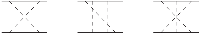
Figure 7: Two- and three-crossed boson exchange contributions to the two-body interaction.

The full expression of the crossed two-boson exchange is taken from ref. [10], where it was put into the form of a dispersion relation appropriate to be used with the Bethe-Salpeter equation, Eq. (1). Among the different expressions given in this work, we retain here that one which is independent of the energy, with $u=0$:

$$K^{(2)}=-\frac{g^{4}}{8\pi^{2}}\int_{4\mu^{2}}^{\infty}\frac{dt^{\prime}}{t^{\prime}-t}\;\sqrt{\frac{t^{\prime}-4\mu^{2}}{t^{\prime}}}\;\;\frac{1}{2\left(\mu^{4}+m^{2}(t^{\prime}-4\mu^{2})\right)}.$$ (37)

Provided that the binding energy is not too large, the other expressions give close results.

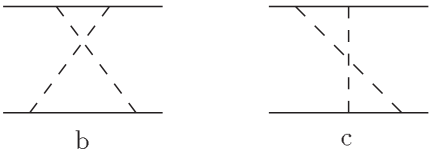
Figure 8: Crossed two-boson exchange contributions to the two-body interaction in time-ordered perturbation theory.

The expressions appropriate for the energy-dependent picture are obtained from the time-ordered diagrams shown in Fig. 8 that have to be added to the box diagram of Fig. 3 a. They read:

$$V^{(2b)}(\vec{p\,},\vec{p}\,^{\prime})=-\frac{g^{4}}{2}\int\frac{d\vec{q}}{(2\pi)^{3}}\;\frac{m}{e_{q}}\frac{m}{e}\;\frac{O_{1}\,(O_{1}\cdot O_{2})\,O_{2}}{\omega\,\omega^{\prime}}\;\frac{m}{e^{\prime}}\frac{m}{e_{q^{\prime}}}\hskip 56.9055pt$$

$$\times\frac{1}{\left(\omega+e+e_{q}-E\right)}\frac{1}{\left(\omega^{\prime}+e^{\prime}+e_{q}-E\right)}\frac{1}{\left(\omega+\omega^{\prime}+e_{q}+e_{q^{\prime}}-E\right)},$$ (38)

$$\rule[0.0pt]{0.0pt}{30.00005pt}V^{(2c)}(\vec{p\,},\vec{p}\,^{\prime})=-\frac{g^{4}}{2}\int\frac{d\vec{q}}{(2\pi)^{3}}\;\frac{m}{e_{q}}\frac{m}{e}\;\frac{O_{1}\,(O_{1}\cdot O_{2})\,O_{2}}{\omega\,\omega^{\prime}}\;\frac{m}{e^{\prime}}\frac{m}{e_{q^{\prime}}}\hskip 56.9055pt$$

$$\times\frac{1}{\left(\omega+e+e_{q}-E\right)}\frac{1}{\left(\omega+e^{\prime}+e_{q^{\prime}}-E\right)}\hskip 56.9055pt$$

$$\times\left\{\frac{1}{\left(\omega+\omega^{\prime}+e+e^{\prime}-E\right)}+\frac{1}{\left(\omega+\omega^{\prime}+e_{q}+e_{q^{\prime}}-E\right)}\right\}.$$ (39)

In addition to the factors defined after Eq. (9), we have used here $e_{q^{\prime}}=\sqrt{m^{2}+\vec{q}\,^{\prime}\,{}^{2}}$ with $\vec{q}\,^{\prime}=\vec{q}-\left(\vec{p}+\vec{p}\,^{\prime}\right)$. Z-type diagrams have a higher order in $\frac{1}{m}$ and are expected to be smaller. They are not incorporated in Eqs. (38, 39). By retaining terms of the lowest order, $\left(\frac{1}{m}\right)^{0}$, one gets the expression of the crossed two-boson exchange that we will include in $V_{eff,sc}^{nr}$ and $V_{eff}^{nr}$. It can be checked that it is equal to the contribution obtained with the dispersion relation, Eq. (37), in the same limit.

For a charged boson, the crossed-box contribution depends on the isospin of the state under consideration. We will consider the case of a state with $T=1$, where it provides further attraction. The effective interaction then reads:

$$V^{nr}_{eff}=V_{0}\;\frac{1+\bar{V}^{(2a)}+\kappa\,(\bar{V}^{(2b)}+\bar{V}^{(2c)})}{1+\bar{V}^{(2a)}+\bar{V}^{(2b)}+\bar{V}^{(2c)}},$$ (40)

where the barred potentials are the same as the ones defined in Eqs. (9, 38, 39) but without the isospin operators $O_{i}$. The factor $\kappa$ is the result of the isospin algebra. For a charged boson, $\kappa=5$, whereas for a neutral boson, $\kappa=1$, in which case the expression greatly simplifies, leaving $V_{0}$ as an effective interaction. Notice that, up to order $\left(\frac{1}{m}\right)^{0}$, this cancellation is expected to hold at all orders in the coupling $g^{2}$, i.e. even including multi-boson exchange diagrams [9]. The effective interaction is thus also given by $V_{0}$ in this case.

4.2 Massive spinless bosons (without and with “charge”)

Table 4: Ground-state binding energies calculated for massive, scalar bosons without and with charge (in units of the constituent mass m), including the box- and the crossed-box contribution. Results for the charged-boson case correspond to a state with total isospin equal to 1. As in the previous section, five cases have been considered: the Bethe-Salpeter equation (B.S.), an energy-dependent model ($V_{E}$), an effective interaction ($V^{nr}_{eff,sc}$), an approximate version of the latter one ($V^{nr}_{eff}$) and, slightly apart, the so-called instantaneous approximation(IA^nr).

$\mu/m$	$\alpha$	${\rm B.S.}$	$V_{E}$	$V^{nr}_{eff,sc}$	$V^{nr}_{eff}$		${\rm IA}^{nr}$
${\rm neutral~{}case}$
	$0.50$	0.013	0.0076	0.0096	0.013		0.013
	$0.75$	0.062	0.027	0.035	0.056		0.056
$.15$	$1.00$	0.158	0.054	0.071	0.129		0.129
	$1.25$	0.324	0.083	0.114	0.233		0.233
	$1.50$	0.593	0.115	0.161	0.367		0.367
	$1.50$	0.077	0.014	0.034	0.093		0.093
	$1.75$	0.162	0.029	0.064	0.180		0.180
$.50$	$2.00$	0.290	0.047	0.101	0.296		0.296
	$2.25$	0.479	0.068	0.143	0.442		0.442
	$2.50$	0.761	0.092	0.189	0.619		0.619
${\rm charged~{}case}$
	$0.30$	0.0062	0.0015	0.0024	0.0095		0.00046
	$0.40$	0.037	0.0083	0.012	0.053		0.0046
$.15$	$0.50$	0.107	0.020	0.028	0.152		0.013
	$0.60$	0.229	0.034	0.049	0.322		0.027
	$0.70$	0.425	0.050	0.073	0.573		0.045
	$0.90$	0.092	0.0007	0.011	0.336		0.0007
	$1.00$	0.183	0.0041	0.023	0.59		0.0052
$.50$	$1.10$	0.319	0.0098	0.040	0.93		0.0138
	$1.20$	0.517	0.0170	0.061	1.36		0.0267

The results for the massive boson case are given in Table 4. As in the ladder approximation, results for the energy-dependent and the non-relativistic self-consistent effective interaction approaches are relatively close to each other in the neutral-boson model. The discrepancy, which tends to increase with the coupling and the boson mass, can be understood as being primarily due to the omission of factors $\sqrt{\frac{m}{e}}$ in the non-relativistic calculation. Taking this into account, it can be considered that the effective self-consistent interaction, $V^{nr}_{eff,sc}$, represents the physics underlying the energy-dependent interaction, $V_{E}$, which it was derived from. However, contrary to the ladder approximation (Table 1), the corresponding results significantly depart from those obtained with the Bethe-Salpeter equation or the (non self-consistent) effective interaction, $V^{nr}_{eff}$, which both are close (or identical) to the results obtained in the instantaneous approximation. It is reminded that the exact equality of the two last columns simply results from the identity, $V_{eff}^{nr}=V_{0}$, which holds for this particular case, see Eq. (40) for $\kappa=1$. We notice here that the discrepancy between the two sets of results tends to increase with the coupling or the boson mass. This feature has a general character in the domain and points to the larger role of higher-order contributions that should show up simultaneously (Z-diagrams or multi-boson exchange).

Discarding results in the instantaneous approximation, those obtained in the charged-boson case show qualitative features similar to the neutral-boson case. Results rather go by pair, $V^{nr}_{eff,sc}$ and $V_{E}$ on one side, B.S. and $V^{nr}_{eff}$ on the other. Relative differencies however are larger. On the one hand, most results are larger than those obtained with the instantaneous approximation. While the latter one was apparently supported by the results for the neutral-boson case, the charged-boson ones show that this approximation is a poor one. On the other hand, a feature evidenced by the examination of Table 4 is the smaller binding energy obtained with the Bethe-Salpeter equation as compared to what is obtained with the effective interaction $V_{eff}^{nr}$. This suggests that the closeness of the corresponding results in the neutral boson case is partly misleading. As mentioned for the ladder approximation, the effective interaction misses attractive contributions due to Z-type diagrams while the Bethe-Salpeter approach involves some renormalization which reduces the attraction. These effects may be roughly equal in the neutral-boson case but could differ substantially in the charged-boson one.

4.3 Discussion

By incorporating the contribution of crossed diagrams, we expected the different approaches, B.S., $V_{E}$, $V_{eff,sc}^{nr}$ and $V_{eff}^{nr}$, to produce a pattern similar to the one evidenced by these models in the ladder approximation. As shown in the previous subsection, this is not the case. An important remark is that, contrary to the ladder approximation, we miss here reliable benchmark results such as the B.S. ones there. The results for the B.S. approach given in Table 4 rely on dispersion relations for calculating the crossed-boson exchange contribution [10]. These ones are well defined within a certain procedure to deal with off-shell effects but this procedure itself is not unique. This prevents one from making a meaningful comparison of the different approaches without entering into a detailed examination. It is only in the case where it has a perturbative character that this examination could be skipped. A different benchmark is that one provided by $V_{eff}^{nr}(={\rm IA}^{nr})$ in the neutral boson case, which can be seen to represent the sum of all contributions at the lowest order $(\frac{1}{m})^{0}$ [9]. A last benchmark is given by the results obtained by Nieuwenhuis and Tjon using the Feynman-Schwinger representation [5]. They incorporate implicitly all contributions of crossed-boson exchanges. In comparison, the crossed-box exchange contribution calculated here with the B.S. equation only explains about half of the total contribution calculated by these authors.

Since $V_{eff}^{nr}$ represents at the same time the sum of all contributions (box and crossed box, see ref. [9]) and the contributions with the range of two-boson exchange (see Eq. (40) for $\kappa=1$), it could be infered that the convergence in terms of the number of exchanged bosons is quickly achieved. This conclusion has an ambiguous character however since accounting for all contributions with the range of three boson exchange also allows one to recover the expected total sum which is nothing but the IA^nr result for $\kappa=1$. A better insight on the role of three, four… boson exchange is provided by the examination of the difference between results obtained with $V_{eff}^{nr}$ and with the self-consistent potential, $V_{eff,sc}^{nr}$. This likely represents an underestimate of the effect however. These extra contributions will reduce the part due to two-boson exchange in the effective interaction. The comparison of results obtained with $V_{eff}^{nr}$ at the order of two-boson exchange, and those obtained with $V_{E}$ provides an estimate on the role of various ingredients entering the calculation: factors $\sqrt{\frac{m}{e}}$ and ($E-e-e^{\prime}$)-corrections in the meson propagators. The large effect prevents one from considering the results obtained with $V_{eff}^{nr}$ as really representative of a complete calculation. This observation is especially important when the comparison is made with results obtained with the B.S. approach, which they roughly agree with, or with those of Nieuwenhuis and Tjon.

At first sight, results obtained with the B.S. approach seem reasonable if they are compared to the FSR results. They leave some room for contributions of three- or multi-boson exchange, which should be roughly equal to the two-boson exchange contribution for the largest couplings for which a comparison is possible. The large discrepancy between our results for the B.S. and $V_{E}$ approaches suggests that the situation is not so simple however. This discrepancy, which should be due in first approximation to Z-type diagrams, is much larger than in the ladder approximation, as shown in Table 1. This may be partly due to the possible proximity of a situation where the binding energy would rapidly increase while the coupling approaches a critical value. More probably, it seems that the dispersion-relation approach does not take fully into account the renormalization effects that $V_{E}$ and $V_{eff,sc}^{nr}$ implicitly incorporate. This situation has some similarity with that one encountered for $V_{eff}^{nr}$, which, for the crossed two-boson exchange, turns out to provide results identical to the instantaneous approximation ones. If correct, the above interpretation would have consequences for approaches based on dispersion relations for calculating crossed-box diagrams. In the simplest case, beside the full three crossed-boson exchange contribution, there should be destructive contributions of the same range, corresponding to the topology (crossed-box $\otimes$ single-boson) exchange.

While the present work was completed, we were informed about different results accounting for the full crossed-boson exchange diagram [35]. These ones are close to those obtained with $V_{E}$ or $V_{eff,sc}^{nr}$, possible discrepancies in the first case being likely due to the contribution of Z-type diagrams omitted here. They tend to support the idea that calculating the crossed-box with dispersion relations is not the best way to provide an estimate of its contribution as soon as the coupling increases. Despite the fact that the obtained values are far from reproducing the FSR results for large couplings, they could still be an overestimate.

5 Conclusion

In this work we investigated different approaches based on the Bethe-Salpeter equation, in particular a 3-dimensional equation with an energy-dependent interaction and a non-relativistic equation with an energy-independent effective interaction. This has been done for the ladder approximation as well as the more complete approach involving crossed-boson exchange with the idea that approximation schemes should not be limited to one of these cases. We especially compared the binding energies for the lowest (normal) states for the case of distinguishable scalar particles with masses for the exchanged boson varying from 0 to $0.5\,m$. This work completes and improves upon another one where the emphasis was rather put on the wave functions obtained from the last two approaches, with and without energy-dependent interactions. Up to departures of relativistic order, we found a strong continuity between the results from different approaches in the ladder approximation. The inclusion of crossed-diagram contributions points to a strong sensitivity to the way the problem is approached.

The reasons why we are able to account in a non-relativistic approach for results of the Bethe-Salpeter equation in the ladder approximation deserve some explanation. The difference between the results obtained with the Bethe-Salpeter equation and those using the instantaneous single-boson exchange approximation in a non-relativistic approach is not due to relativity, as sometimes advocated, but to the fact that the latter misses the field-theory character underlying the former. Since a field-theory can be dealt with in a non-relativistic scheme, it should be no surprise that one is able to get rid of the above difference. The so-called instantaneous approximation, often employed to provide some non-relativistic interaction, simply represents a too naive view of what the interaction in a non-relativistic picture should be, missing many-body effects in its determination. Contrary to a common belief, the dynamics involving the relative time variable can be accounted for partly, if not totally, in a three-dimensional approach, in a way which is not Lorentz-covariant however. The main effect in the small coupling limit, which implies corrections with the range of multi-boson exchange, is a renormalization of the so-called instantaneous interaction by the probability of having two constituents only. Since in the ladder-approximation, the part with in-flight bosons plays no role, the force turns out to be effectively weakened. This is one of the most intuitive effects one can think of. The intensity of the force being smaller, it becomes easier for a self-consistent, non-relativistic approach to account for effects obtained in a relativistic one. The improvement we introduced in calculating the effective interaction is quite significant. While it removes partly the agreement with more elaborate calculations achieved in some cases, we believe that the effect is fully relevant. This points to ingredients missing in the effective interaction, especially those in relation with non-locality effects, which are obviously more difficult to incorporate.

We also looked at the contribution due to crossed two-(massive) boson exchange. This exchange represents an essential improvement upon the ladder approximation, which offers interest with certain respects but remains academic with other ones. The effects are generally quite large, especially in the case of charged-boson exchange where one should be seriously concerned by higher order crossed-boson exchange contributions. In any case, this casts serious doubts on the possibility to reliably describe physical systems in the strong-interaction regime by only retaining one-boson exchange contributions. This could be however partly remedied by fitting parameters of a certain model, when possible, as it is done for the NN interaction models. In view of these large effects, the fact that, in some cases, we recover more or less the results of the so-called instantaneous approximation for the neutral-boson exchange should be considered with a lot of caution. This result is obtained because the contribution of the crossed two-boson exchange, most often neglected, has been included consistently with the box two-boson exchange contribution. Such a result may have a more general character and be simply due to the fact that, for neutral, spinless-boson exchange, the interaction, supposed to be given by the instantaneous approximation, is the same for components with an undetermined number of accompanying bosons and, therefore, transparent to the presence of bosons in flight. By no means, one can draw an argument from this result in favor of the validity of the one-boson exchange contribution in the non-relativistic approach.

This conclusion is supported by another feature of our results. The binding energies calculated with the Bethe-Salpeter equation and the effective interaction are significantly smaller than the completely non-perturbative ones obtained by Nieuwenhuis and Tjon [5] (a factor of 2 at $\alpha\simeq 0.9$), indicating the existence of further sizeable corrections of higher order [10]. Most probably, the closeness of our results for the Bethe-Salpeter equation and the effective interaction, which was obtained in a few cases, is partly accidental, as already mentioned above. Those with the effective interaction miss contributions of relativistic order, like Z-type diagrams, while the Bethe-Salpeter equation, where these ones are included, does not take into account contributions with a higher number of exchanged bosons. The accidental character of the closeness of these different results is further supported by the examination of those we obtained for the charged boson case.

We presented results for zero-mass bosons only in the ladder approximation. Some results were obtained for the crossed-boson exchange diagram but they did not evidence any striking difference with the $\mu=0.15\,m$ case. These results need to be more elaborated, especially in view of possible applications to the photon or gluon case. The cancellation between the renormalization of the instantaneous approximation interaction and the effect of the crossed-boson exchange, which is expected in the massive neutral-boson case at order $\left(\frac{1}{m}\right)^{0}$, and has been partly obtained in our calculations, is more difficult to be achieved in the zero-mass case. For small couplings, the corrections to the binding energies that are dominated by the term $\frac{\alpha^{2}}{4n^{2}}$ are of the order $\alpha^{3}\,\log(c\alpha)$ [11], while the total correction is expected to be of order $\alpha^{4}$. The reason is that solving a certain integral equation allows one to sum up an infinite set of contributions with increasing order, but also an increasingly divergent character in the infra-red limit. This prevents one from reproducing numerically the above expected cancellation without considering an infinite set of selected crossed-boson exchanges, having similar properties. From present results and further studies performed separately, it seems that the convergence to the full result is likely to be slow for couplings of the order $\alpha\simeq 1$.

All studies presented here have been performed in a model involving scalar particles only. This greatly simplifies the discussions by providing a better insight on the origin of various corrections (renormalization of the instantaneous approximation interaction, relativistic corrections,….). Despite the fact that the model is not an especially realistic one, we nevertheless believe that our conclusions have some general character. The most important one is probably the very limited validity range of the instantaneous one-boson exchange approximation which, strictly speaking, is valid only for small energy transfers and therefore only makes sense for the Born amplitude in the non-relativistic regime. Its apparent success in QED or in hadronic physics is largely misleading. It rather points to large contributions from multi-boson exchanges. In the case of QED, they are required to recover the Coulomb potential as is well known, whereas in hadronic physics, they provide a more microscopic description of the forces, most often simulated by instantaneous exchanges of single bosons with fitted parameters.

Acknowledgements We are indebted to E. Moulin and N. Ploquin, whose work on non-locality effects provided useful insight on their role in the context of the present work. We are also grateful to D. Phillips for providing results concerning the contribution of the crossed-box diagram.

Appendix A The box diagram

We give here the analytic result for the box diagram of Fig. 3 a, in the case where the factors $\frac{m}{e_{q}}$ and terms like $E-e-e^{\prime}$ in the denominator of Eq. (9) are neglected. It is not what we actually used in the calculations presented in this work but it turned out to be quite useful for numerical tests. The (energy-independent) expression for $V^{(2a)}(\vec{p\,},\vec{p}\,^{\prime})$ then takes the form

$$V^{(2a)}(\vec{p\,},\vec{p}\,^{\prime})=-\frac{1}{2}\int\frac{d\vec{q}}{(2\pi)^{3}}\;\frac{m}{e}\left(\frac{g^{4}\;(O_{1}\,O_{2})\,(O_{1}\,O_{2})}{\omega\,\omega^{\prime}\;(\omega+\omega^{\prime})}\;\;\frac{1}{\omega\,\omega^{\prime}}\right)\frac{m}{e^{\prime}},$$ (41)

with the definitions $\omega=\sqrt{\mu^{2}+(\vec{p}-\vec{q}\,)^{2}}$, $\omega^{\prime}=\sqrt{\mu^{2}+(\vec{p}\,^{\prime}-\vec{q}\,)^{2}}$, $e=\sqrt{m^{2}+\vec{p}^{\,2}}$ and $e^{\prime}=\sqrt{m^{2}+\vec{p}\,^{\prime\,2}}$. If one defines the integral $I$ by

$$V^{(2a)}(\vec{p\,},\vec{p}\,^{\prime})=:-\frac{1}{2}\frac{m^{2}}{ee^{\prime}}\frac{g^{4}}{(2\pi)^{3}}(O_{1}\,O_{2})\,(O_{1}\,O_{2})\,I,$$ (42)

then it is found that

$$I = \int\frac{d\vec{q}}{\left[\mu^{2}+(\vec{p}-\vec{q})^{2}\right]\left[\mu^{2}+(\vec{p}\,^{\prime}-\vec{q})^{2}\right]\left[\sqrt{\mu^{2}+(\vec{p}-\vec{q})^{2}}+\sqrt{\mu^{2}+(\vec{p}\,^{\prime}-\vec{q})^{2}}\right]}$$

$$= \frac{2\pi}{k}\int_{0}^{\infty}\frac{q\;dq}{\left(\mu^{2}+q^{2}\right)^{\frac{3}{2}}}\log\frac{\sqrt{\mu^{2}+(k+q)^{2}}\left[\sqrt{\mu^{2}+q^{2}}+\sqrt{\mu^{2}+(k-q)^{2}}\right]}{\sqrt{\mu^{2}+(k-q)^{2}}\left[\sqrt{\mu^{2}+q^{2}}+\sqrt{\mu^{2}+(k+q)^{2}}\right]},$$

where $k=|\vec{k}|=|\vec{p}-\vec{p}\,^{\prime}|$. From this form one derives the following analytical properties of the integral $I$:

$$I=\frac{2\pi}{3\mu^{2}}\hskip 28.45274pt\;\;\; {\rm if} \;\;\vec{k}=0,$$

$$I=\frac{2\pi}{k^{2}}\;4\log 2\;\;\; {\rm if} \;\;\mu=0,$$ (44)

$$I\rightarrow\frac{2\pi}{k^{2}}\;4\log 2\;\;\; {\rm for} \;\;k\rightarrow\infty.$$

Integrating by parts, one finds the following expression for $I$:

$$I = \frac{2\pi}{k\sqrt{k^{2}+4\mu^{2}}}\left\{\frac{2}{\sqrt{1-c}}\log\frac{1+\sqrt{1-c}}{1-\sqrt{1-c}}\right.$$ (45)

$$\hskip 85.35826pt\left.-4\sqrt{\frac{c}{1-c}}\arctan\sqrt{\frac{1-c}{c}}+2\log c\right\},$$

where the factor $c$ is given by

$$c=\frac{\sqrt{k^{2}+4\mu^{2}}-k}{\sqrt{k^{2}+4\mu^{2}}+k}.$$ (46)

A careful analysis reveals that the expression of Eq. (45) satisfies the conditions of Eqs. (44), because of a cancellation of divergencies in single terms.

References

- [1] E.E. Salpeter and H.A. Bethe, Phys. Rev. 84 (1951) 1232.
- [2] B. Silvestre-Brac, A. Bilal, C. Gignoux, P. Schuck, Phys. Rev. D 29 (1984) 2275.
- [3] A. Bilal, P. Schuck, Phys. Rev. D 31 (1985) 2045.
- [4] D.R. Phillips, S.J. Wallace, Phys. Rev. C 54 (1996) 507.
- [5] T. Nieuwenhuis, J.A. Tjon, Phys. Rev. Lett. 77 (1996) 814.
- [6] T. Frederico, J.H.O. Sales, B.V. Carlson, P.U. Sauer, Few-Body Systems Suppl. 10 (1999) 123.
- [7] J. Bijtebier, Nucl. Phys. A 623 (1997) 498.
- [8] J.W. Darewych, Can. J. Phys. 76 (1998) 523.
- [9] A. Amghar, B. Desplanques, Few-Body Systems 28 (2000) 65.
- [10] L. Theußl, B. Desplanques, nucl-th/9908007, to appear in Few-Body Systems.
- [11] G. Feldman, T. Fulton, J. Townsend, Phys. Rev. D 7 (1973) 1814.
-
[12]
I.T. Todorov, Phys. Rev. D 3 (1971) 2351;
E. Brezin, C. Itzykson , J. Zinn-Justin, Phys. Rev. D1 (1970) 2349;
F. Gross, Phys. Rev. C 26 (1982) 2203;
A.R. Neghabian, W. Glöckle, Can. J. Phys. 61 (1983) 85;
C. Itzykson, J.B. Zuber, Quantum Field Theory. McGraw-Hill International Editions (1985). - [13] J.L. Friar, Phys. Rev. C 22 (1980) 796.
-
[14]
G.C. Wick, Phys. Rev. 96 (1954) 1124;
R.E. Cutkosky, Phys. Rev. 96 (1954) 1135. -
[15]
N. Fukuda, K. Sawada, M. Taketani,
Prog. Theor. Phys. 12 (1954) 156;
S. Okubo, Prog. Theor. Phys. 12 (1954) 603;
M. Sugawara, S. Okubo, Phys. Rev. 117 (1960) 605. - [16] R.K. Bhaduri, M. Brack, Phys. Rev. 25 (1982) 1443.
- [17] G.P. Lepage, nucl-th/9706029.
- [18] A. Klein, Phys. Rev. 90 (1953) 1101.
- [19] R. Machleidt, K. Holinde, Ch. Elster, Phys. Rep. 149 (1987) 1.
-
[20]
B. Desplanques, Phys. Lett. 203 B (1988) 200;
B. Desplanques, In: Trends in Nuclear Physics, 100 years later, les Houches LXVI (1996); H. Nifenecker et al. (eds.). North-Holland (1998). - [21] F.G. Perey, D.S. Saxon, Phys. Lett. 10 (1964) 107.
- [22] A.D. Lahiff, I.R. Afnan, Phys. Rev. C 56 (1997) 2387.
- [23] P. Ring, P. Schuck, The Nuclear Many-Body Problem, Springer Verlag (1980).
- [24] C. Mahaux, P.F. Bortignon, R.A. Broglia, C.H. Dasso, Phys. Rep. 120 (1985) 1.
- [25] M. Chemtob, J.W. Durso, D.O. Riska, Nucl. Phys. B 38 (1972) 141.
- [26] M. Lacombe, B. Loiseau, J.M. Richard, R. Vinh Mau, J. Côté, P. Pirés, R. de Tourreil, Phys. Rev. C 21 (1980) 861.
- [27] F. Gross, Phys. Rev. 186 (1969) 1448.
-
[28]
R. Blankenbecler, R. Sugar,
Phys. Rev. 142 (1966) 1051;
A.A. Logunov, A.N. Tavkhelidze, Nuovo Cimento 29 (1963) 380. - [29] M. Chemtob, in: Mesons in Nuclei, Eds. M.Rho and D.H. Wilkinson, North-Holland Publishing Company, 1979.
- [30] A.A. Khelashvili, G.A. Khelashvili, N. Kiknadze, T.P. Nadareishvili, quant-ph/9907078.
- [31] B. Baumgartner, H. Grosse, A. Martin, Phys. Lett 146 B (1984) 363; Nucl. Phys. B 254 (1985) 528.
- [32] C.R. Ji, R.J. Furnstahl, Phys. Lett. 167 B (1986) 11.
- [33] Ch. Elster, E.E. Evans, H. Kamada, W. Glöckle, Few-Body Systems 21 (1996) 25.
- [34] M. Mangin-Brinet, J. Carbonell, Phys. Lett. B 474 (2000) 237.
-
[35]
J.A. Tjon, private communication;
I.R. Afnan and D.R. Phillips, private communication.