MKPH-T-00-23
The E2/M1 and C2/M1 ratios and form factors in $N\rightarrow\Delta$ transitions

Abstract

A partial wave analysis of pion photoproduction has been obtained in the framework of fixed-$t$ dispersion relations valid from threshold up to 500 $MeV$. In the resonance region we have precisely determined the electromagnetic properties of the $\Delta(1232)$ resonance, in particular the E2/M1 ratio $R_{EM}=(-2.5\pm 0.1)\%$. For pion electroproduction recent experimental data from Mainz, Bates and JLab for $Q^{2}$ up to 4.0 (GeV/c)² have been analyzed with two different models, an isobar model (MAID) and a dynamical model. The E2/M1 ratios extracted with these two models show, starting from a small and negative value at the real photon point, a clear tendency to cross zero, and become positive with increasing $Q^{2}$. This is a possible indication of a very slow approach toward the pQCD region. The C2/M1 ratio near the photon point is found as $R_{SM}(0)=(-6.5\pm 0.5)\%$. At high $Q^{2}$ the absolute value of the ratio is strongly increasing, a further indication that pQCD is not yet reached.

1 INTRODUCTION

The determination of the quadrupole excitation strength $E_{1+}^{(3/2)}$ in the region of the $\Delta(1232)$ resonance has been the aim of considerable experimental and theoretical activities. Within the harmonic oscillator quark model, the $\Delta$ and the nucleon are both members of the symmetrical 56-plet of $SU(6)$ with orbital momentum $L=0$, positive parity and a Gaussian wave function in space. In this approximation the $\Delta$ may only be excited by a magnetic dipole transition $M_{1+}^{(3/2)}$ [1]. However, in analogy with the atomic hyperfine interaction or the forces between nucleons, also the interactions between the quarks contain a tensor component due to the exchange of gluons. This hyperfine interaction admixes higher states to the nucleon and $\Delta$ wave functions, in particular $d$-state components with $L=2$, resulting in a small electric quadrupole transition $E_{1+}^{(3/2)}$ between nucleon and $\Delta$ [2, 3, 4]. In addition quadrupole transitions are possible by mesonic and gluonic exchange currents [5]. Therefore an accurate measurement of $E_{1+}^{(3/2)}$ is of great importance in testing the forces between the quarks and, quite generally, models of nucleons and isobars.

The E2/M1 ratio, $R_{EM}=E_{1+}^{(3/2)}/M_{1+}^{(3/2)}$ has been predicted to be in the range $-3\%\leq R_{EM}<0\%$ in the framework of constituent quark [2, 4, 5, 6], relativized quark [7, 8] and chiral bag models [9]. Considerably larger values have been obtained in Skyrme models [10]. A first lattice QCD calculation resulted in a small value with large error bars $(-6\%\leq R_{EM}\leq 12\%)$ [11]. However, the connection of the model calculations with the experimental data is not evident. Clearly, the $\Delta$ resonance is coupled to the pion-nucleon continuum and final-state interactions will lead to strong background terms seen in the experimental data, particularly in case of the small $E_{1+}$ amplitude. The question of how to ”correct” the experimental data to extract the properties of the resonance has been the topic of many theoretical investigations. Unfortunately it turns out that the analysis of the small $E_{1+}$ amplitude is quite sensitive to details of the models, e.g. nonrelativistic vs. relativistic resonance denominators, constant or energy-dependent widths and masses of the resonance, sizes of the form factor included in the width etc. In other words, by changing these definitions the meaning of resonance vs. background changes, too.

In order to study the $\Delta$ deformation, pion photoproduction on the proton has been measured by the LEGS collaboration [12] at Brookhaven and by the A2 collaboration [13] at Mainz using transversely polarized photons, i.e. by measuring the polarized photon asymmetry $\Sigma$. In particular, the cross section $d\sigma_{\parallel}$ for photon polarization in the reaction plane turns out to be very sensitive to the small $E_{1+}$ amplitude. Assuming for simplicity that only the $P$-wave multipoles contribute, the differential cross section is

$$\frac{d\sigma_{\parallel}}{d\Omega}=\frac{q}{k}(A_{\parallel}+B_{\parallel}\cos\Theta_{\pi}+C_{\parallel}\cos^{2}\Theta_{\pi}),$$ (1)

where $q$ and $k$ are the pion and photon momenta and $\Theta_{\pi}$ is the pion emission angle in the $c.m.$ frame. Neglecting the (small) contributions of the Roper multipole $M_{1-}$, one obtains [13]

$$C_{\parallel}/A_{\parallel}\approx 12R_{EM},$$ (2)

because the isospin $\frac{3}{2}$ amplitudes strongly dominate the cross section for $\pi^{0}$ production.

In order to obtain the C2/M1 ratio and the form factors as functions of $Q^{2}$ pion electroproduction has been studied. At Mainz, Bonn, Bates and JLab different experiments have been performed, without polarization as well as single and double polarization.

While the experiments at Mainz and Bates measured at $Q^{2}\sim 0.1$ GeV² in order to get the C2/M1 ratio close to the photon point, the JLab experiment was motivated by the possibility of determining the range of momentum transfers where perturbative QCD (pQCD) would become applicable. In the limit of $Q^{2}\rightarrow\infty$, pQCD predicts [14] that only helicity-conserving amplitudes contribute, leading to $R_{EM}=E_{1+}^{(3/2)}/M_{1+}^{(3/2)}\rightarrow 1$ and $R_{SM}=S_{1+}^{(3/2)}/M_{1+}^{(3/2)}\rightarrow const$.

2 PION PHOTOPRODUCTION

Starting from fixed-$t$ dispersion relations for the invariant amplitudes of pion photoproduction, the projection of the multipole amplitudes leads to a well known system of integral equations,

$$\mbox{Re}{\cal M}_{l}(W)={\cal M}_{l}^{\mbox{\scriptsize P}}(W)+\frac{1}{\pi}\sum_{l^{\prime}}{\cal P}\int_{W_{\mbox{\scriptsize thr}}}^{\infty}K_{ll^{\prime}}(W,W^{\prime})\mbox{Im}{\cal M}_{l^{\prime}}(W^{\prime})dW^{\prime},$$ (3)

where ${\cal M}_{l}$ stands for any of the multipoles $E_{l\pm},M_{l\pm},$ and ${\cal M}_{l}^{\mbox{\scriptsize P}}$ for the corresponding (nucleon) pole term. The kernels $K_{ll^{\prime}}$ are known, and the real and imaginary parts of the amplitudes are related by unitarity. In the energy region below two-pion threshold, unitarity is expressed by the final state theorem of Watson,

$${\cal M}_{l}^{I}(W)=\mid{\cal M}_{l}^{I}(W)\mid e^{i(\delta_{l}^{I}(W)+n\pi)},$$ (4)

where $\delta_{l}^{I}$ is the corresponding $\pi N$ phase shift and $n$ an integer. We have essentially followed the method of Schwela et al [15, 16] to solve Eq. (3) with the constraint (4). In addition we have taken into account the coupling to some higher states neglected in that earlier reference. At the energies above two-pion threshold up to $W=2$ GeV, Eq. (4) has been replaced by an Ansatz based on unitarity [15]. Finally, the contribution of the dispersive integrals from $2$ GeV to infinity has been replaced by $t$-channel exchange, parametrized by certain fractions of $\rho$- and $\omega$-exchange. Furthermore, we have to allow for the addition of solutions of the homogeneous equations to the coupled system of Eq. (3). The whole procedure introduces 9 free parameters, which have been determined by a fit to the data. [17]

In Figure 1 we show the $P_{33}$ multipoles $M^{3/2}_{1+}$ and $E^{3/2}_{1+}$. Our dispersion theoretical analysis (solid line) agrees very well with our single-energy fit and with the single-energy fit of Beck et al. [18]. The only systematic deviation becomes visible in the electric multipole above the resonance position. This can be due either to our truncation of partial waves or to systematics in the experiment at the highest energies. In a new experiment a full angular coverage of the differential cross section for $p(\gamma,\pi^{0})p$ over a wide range of energy from threshold up to $E^{lab}_{\gamma}=440MeV$ has been taken and in the near future a new and very precise multipole analysis should also clarify this small deviation.

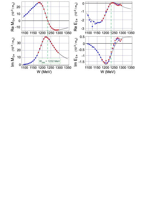
Figure 1: $P_{33}$ amplitudes $M_{1+}^{3/2}$ and $E_{1+}^{3/2}$ for pion photoproduction in the $\Delta(1232)$ region. The black points are our single-energy fits, the grey points are taken from Beck et al. [18]. In most cases they exactly overlap.

According to the Watson theorem, at least up to the two-pion threshold, the ratio $E_{1+}^{(3/2)}/M_{1+}^{(3/2)}$ is a real quantity. However, it is not a constant but even a rather strongly energy dependent function. If we determine the resonance position as the point, where the phase $\delta_{1+}^{(3/2)}(W=M_{\Delta})=90^{\circ}$, we can define the so-called ”full” ratio

$$R_{EM}=\left.\frac{E_{1+}^{(3/2)}}{M_{1+}^{(3/2)}}\right|_{W=M_{\Delta}}=\left.\frac{\mbox{Im}E_{1+}^{(3/2)}}{\mbox{Im}M_{1+}^{(3/2)}}\right|_{W=M_{\Delta}}\,.$$ (5)

We note that this ratio is identical to the ratio obtained with the $K$-matrix at the $K$-matrix pole $W=M_{\Delta}$. This can be seen by using the relation between the $T$- and the $K$-matrix,

$$T=K\cos\delta e^{i\delta}\quad\mbox{and consequently}\quad K=\mbox{Re}T+\mbox{Im}T\,tan\delta\,.$$ (6)

Therefore, at $W=M_{\Delta}$ we find

$$K(E_{1+}^{(3/2)})/K(M_{1+}^{(3/2)})=\mbox{Im}E_{1+}^{(3/2)}/\mbox{Im}M_{1+}^{(3/2)}=R_{EM}\,.$$ (7)

The recent, nearly model-independent value of the Mainz group at $W=M_{\Delta}=1232$ MeV is $(-2.5\pm 0.1\pm 0.2)\%$ [18] is in excellent agreement with our dispersion theoretical calculation that gives $(-2.54\pm 0.10)\%$, see Table 1.

Table 1: E2/M1 ratios for $Q^{2}$=0 from different analyses.

$R_{EM}[\%]$	Reference
$-2.54\pm 0.10$	Hanstein et al. [17]
$-2.5\pm 0.1_{stat.}\pm 0.2_{syst.}$	Beck et al. [18]
$-3.0\pm 0.3_{stat.+syst.}\pm 0.2_{mod.}$	Blanpied et al. [12]
$-1.5\pm 0.5$	Arndt et al. [19]
$-3.19\pm 0.24$	Davidson et al. [20]
$-2.5\pm 0.5$	PDG 2000 estimate [21]

As it was demonstrated in different approaches [17, 22], the precise E2/M1 ratio is very sensitive to the specific database used in the fit. Therefore, the SAID value, obtained with the full database is rather low ($-1.5\%$) and the values obtained with the LEGS differential cross sections are twice as large, around $-3\%$.

The ratio so far discussed above, is the ratio at the K-matrix pole on the real energy axis. In scattering theory, the T-matrix pole in the complex plane, however, is more fundamental. The analytic continuation of a resonant partial wave as function of energy into the second Riemann sheet should generally lead to a pole in the lower half-plane. A pronounced narrow peak reflects a time-delay in the scattering process due to the existence of an unstable excited state. This time-delay is related to the speed $SP$ of the scattering amplitude $T$, defined by [23]

$$SP(W)=\left|\frac{dT(W)}{dW}\right|,$$ (8)

where $W$ is the total $c.m.$ energy. In the vicinity of the resonance pole, the energy dependence of the full amplitude $T=T_{B}+T_{R}$ is determined by the resonance contribution,

$$T_{R}(W)=\frac{r\Gamma_{R}e^{i\phi}}{M_{R}-W-i\Gamma_{R}/2}\,\,,$$ (9)

while the background contribution $T_{B}$ should be a smooth function of energy, ideally a constant. We note in particular that $W_{R}=M_{R}-i\Gamma_{R}/2$ indicates the position of the resonance pole in the complex plane, i.e. $M_{R}$ and $\Gamma_{R}$ are constants and differ from the energy-dependent widths, and possibly masses, derived from fitting certain resonance shapes to the data. In the limit where the derivative of the smooth background can be neglected, the speed takes the simple form

$$SP(W)=\frac{r\Gamma_{R}}{(M_{R}-W)^{2}+\Gamma_{R}^{2}/4}\,.$$ (10)

From this form, the position of the pole as well as the absolute magnitude of the residue can be easily obtained. Furthermore, in our dispersion approach we have also checked the validity of the assumption to neglect the background and found that this procedure works very well for the Delta resonance.

Applying this technique to our $P_{33}$ amplitudes we find the pole at $W_{R}=M_{R}-i\Gamma_{R}/2=(1211-50i)$ MeV in excellent agreement with the results obtained from $\pi N$ scattering, $M_{R}=(1210\pm 1)$ MeV and $\Gamma_{R}=100$ MeV [23]. The complex residues and the phases are obtained as $r_{E}=1.23\cdot 10^{-3}/m_{\pi},\phi_{E}=-154.7^{\circ},r_{M}=21.16\cdot 10^{-3}/m_{\pi}$ and $\phi_{M}=-27.5^{\circ}$, yielding a complex ratio of the residues

$$R_{\Delta}=\frac{r_{E}e^{i\phi_{E}}}{r_{M}e^{i\phi_{M}}}=-0.035-0.046i.$$ (11)

While the experimentally observed ratio $R_{EM}$ is real and very sensitive to small changes in energy, the ratio $R_{\Delta}$ is a complex number defined by the residues at the pole, therefore, it does not depend on energy.

It should be noted, however, that a resonance without the accompanying background terms is unphysical, in the sense that only the sum of the two obeys unitarity. Furthermore we want to point out that the speed-plot technique does not give information about the strength parameters of a ”bare” resonance, i.e. in the case where the coupling to the continuum is turned off. Both the pole position and the residues at the pole will change for such a hypothetical case, but the exact values for the ”bare” resonance can only be determined by a model calculation and as such will depend on the ingredients of the model.

3 PION ELECTROPRODUCTION

In the dynamical approach to pion photo- and electroproduction [24], the t-matrix is expressed as

$$t_{\gamma\pi}(E)=v_{\gamma\pi}+v_{\gamma\pi}\,g_{0}(E)\,t_{\pi N}(E)\,,$$ (12)

where $v_{\gamma\pi}$ is the transition potential operator for $\gamma^{*}N\rightarrow\pi N$, and $t_{\pi N}$ and $g_{0}$ denote the $\pi N$ t-matrix and free propagator, respectively, with $E\equiv W$ the total energy in the CM frame. A multipole decomposition of Eq. (12) gives the physical amplitude in channel $\alpha$ [24],

$$t_{\gamma\pi}^{(\alpha)}(q_{E},k;E+i\epsilon) = \exp{(i\delta^{(\alpha)})}\,\cos{\delta^{(\alpha)}}$$ (13)

$$\times \left[v_{\gamma\pi}^{(\alpha)}(q_{E},k)+P\int_{0}^{\infty}dq^{\prime}\frac{q^{\prime 2}R_{\pi N}^{(\alpha)}(q_{E},q^{\prime};E)\,v_{\gamma\pi}^{(\alpha)}(q^{\prime},k)}{E-E_{\pi N}(q^{\prime})}\right],$$

where $\delta^{(\alpha)}$ and $R_{\pi N}^{(\alpha)}$ are the $\pi N$ scattering phase shift and reaction matrix in channel $\alpha$, respectively; $q_{E}$ is the pion on-shell momentum and $k=|{\bf k}|$ is the photon momentum. The multipole amplitude in Eq. (13) manifestly satisfies the Watson theorem and shows that the $\gamma\pi$ multipoles depend on the half-off-shell behavior of the $\pi N$ interaction.

In a resonant channel like (3,3) in which the $\Delta(1232)$ plays a dominant role, the transition potential $v_{\gamma\pi}$ consists of two terms,

$$v_{\gamma\pi}(E)=v_{\gamma\pi}^{B}+v_{\gamma\pi}^{\Delta}(E)\,,$$ (14)

where $v_{\gamma\pi}^{B}$ is the background transition potential and $v_{\gamma\pi}^{\Delta}(E)$ corresponds to the contribution of the bare $\Delta$.

It is well known that for a correct description of the resonance contributions we need, first of all, a reliable description of the nonresonant part of the amplitude.

In the new version of MAID (MAID2000), the $S$, $P$, $D$ and $F$ waves of the background contributions are complex numbers defined in accordance with the K-matrix approximation,

$$t_{\gamma\pi}^{B,\alpha}({\rm MAID})=\exp{(i\delta^{(\alpha)})}\,\cos{\delta^{(\alpha)}}v_{\gamma\pi}^{B,\alpha}(W,Q^{2}).$$ (15)

From Eqs. (13) and (15), one finds that the difference between the background terms of MAID and of the dynamical model is that off-shell rescattering contributions (principal value integral) are not included in MAID. To take account of the inelastic effects at the higher energies, we replace $\exp{(i\delta^{(\alpha)})}\cos{\delta^{(\alpha)}}=\frac{1}{2}(\exp{(2i\delta^{(\alpha)})}+1)$ in Eqs. (13) and (15) by $\frac{1}{2}(\eta_{\alpha}\exp{(2i\delta^{(\alpha)})}+1)$, where $\eta_{\alpha}$ is the inelasticity. In our actual calculations, both the $\pi N$ phase shifts $\delta^{(\alpha)}$ and inelasticity parameters $\eta_{\alpha}$ are taken from the analysis of the GWU group [19].

Following Ref. [25], we assume a Breit-Wigner form for the resonance contribution ${\cal A}^{R}_{\alpha}(W,Q^{2})$ to the total multipole amplitude,

$${\cal A}_{\alpha}^{R}(W,Q^{2})\,=\,{\bar{\cal A}}_{\alpha}^{R}(Q^{2})\,\frac{f_{\gamma R}(W)\Gamma_{R}\,M_{R}\,f_{\pi R}(W)}{M_{R}^{2}-W^{2}-iM_{R}\Gamma_{R}}\,e^{i\phi},$$ (16)

where $f_{\pi R}$ is the usual Breit-Wigner factor describing the decay of a resonance $R$ with total width $\Gamma_{R}(W)$ and physical mass $M_{R}$. The expressions for $f_{\gamma R},\,f_{\pi R}$ and $\Gamma_{R}$ are given in Ref. [25]. The phase $\phi(W)$ in Eq. (16) is introduced to adjust the phase of the total multipole to equal the corresponding $\pi N$ phase shift $\delta^{(\alpha)}$. Because $\phi=0$ at resonance, $W=M_{R}$, this phase does not affect the $Q^{2}$ dependence of the $\gamma NR$ vertex.

In the dynamical model of Ref. [26], a scaling assumption was made concerning the (bare) form factors ${\bar{\cal A}}_{\alpha}^{\Delta}(Q^{2})$, namely, that all of them have the same $Q^{2}$ dependence,

$${\bar{\cal A}}_{\alpha}^{\Delta}(Q^{2})={\bar{\cal A}}_{\alpha}^{\Delta}(0)\frac{k}{k_{W}}\,F(Q^{2}),\,$$ (17)

where $\alpha=M,E,$ and $S$, $k_{W}=(W^{2}-m_{N}^{2})/2W$, ${k}^{2}=Q^{2}+((W^{2}-m_{N}^{2}-Q^{2})/2W)^{2}$, and $F$ is normalized to $F(0)=1$. The values of ${\bar{\cal A}}_{M}^{\Delta}(0)$ and ${\bar{\cal A}}_{E}^{\Delta}(0)$ were determined by fitting to the multipoles obtained in the recent analyses of the Mainz [17] and GWU [27] groups. The $Q^{2}$ evolution of the form factor $F$ was assumed to take the form $F(Q^{2})=(1+\beta\,Q^{2})\,e^{-\gamma Q^{2}}\,G_{D}(Q^{2}),$ where $G_{D}(Q^{2})=1/(1+Q^{2}/0.71)^{2}$ is the usual dipole form factor. The parameters $\beta$ and $\gamma$ were determined by fitting ${\bar{\cal A}}_{M}^{\Delta}(Q^{2})$ to the data for $G_{M}^{*}$ defined by [25, 26],

$$M_{1+}^{(3/2)}(M_{\Delta},Q^{2})=\frac{k}{m_{N}}\sqrt{\frac{3\alpha_{em}}{8\Gamma_{exp}q_{\Delta}}}\,G_{M}^{*}(Q^{2}),$$ (18)

where $\alpha_{em}=1/137$, $\Gamma_{exp}=115$ MeV, and $q_{\Delta}$ is the pion momentum at $W=M_{\Delta}$. With the relation ${\bar{\cal A}}_{E}^{\Delta}(0)={\bar{\cal A}}_{S}^{\Delta}(0)$, the ratios $R_{EM}$ and $R_{SM}$ between the full multipoles were then evaluated [26] and found to agree with the values extracted in Ref. [28].

In the present analysis, we do not impose the scaling assumption and write, for electric ($\alpha=E$) and Coulomb ($\alpha=S$) multipoles,

$${\bar{\cal A}}_{\alpha}^{\Delta}(Q^{2})=X_{\alpha}^{\Delta}(Q^{2})\,{\bar{\cal A}}_{\alpha}^{\Delta}(0)\frac{k}{k_{W}}\,F(Q^{2}),$$ (19)

with $X_{\alpha}^{\Delta}(0)=1$, and we allow both $X_{E}$ and $X_{S}$ to be determined by the experiment.

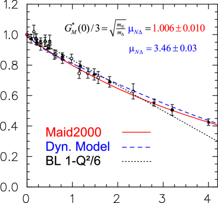
Figure 2: The $Q^{2}$ dependence of the magnetic $N\rightarrow\Delta$ transition form factor $G_{M}^{*}$ divided by three times the nucleon dipole form factor. The solid and dashed curves are the results of the MAID and dynamical model analyses, respectively. The dotted line shows the simple fit of Ref. [29]. The data at $Q^{2}$=2.8 and 4.0 $(GeV/c)^{2}$ are from Ref. [28]. For other data see Ref. [33].

The dynamical model and MAID are used to analyze the recent JLab differential cross section data on $p(e,e^{\prime}p)\pi^{0}$ at high $Q^{2}$. All measured data, 751 points at $Q^{2}$=2.8 and 867 points at $Q^{2}$=4.0 (GeV/c)² covering the entire energy range $1.1<W<1.4$ GeV, are included in our global fitting procedure using the MINUIT code and we obtain a very good fit to the measured differential cross sections. Our results for the $G_{M}^{*}$ form factor are shown in Figure 2. Here the best fit is obtained with $\gamma=0.21$ (GeV/c)^-2 and $\beta=0$ in the case of MAID, and $\gamma=0.40$ (GeV/c)^-2 and $\beta=0.52$(GeV/c)^-2 in the case of the dynamical model. It is worth noting that in the definition of Eq. (18), $G_{M}^{*}(0)/3$ takes a value of 1 to an accuracy of $1\%$. This very precise value is extracted from the recent Mainz experiment [18]. With this number we can also determine a very precise $N\rightarrow\Delta$ magnetic transition moment, $\mu_{N\Delta}=3.46\pm 0.03$ in units of nuclear magnetons.

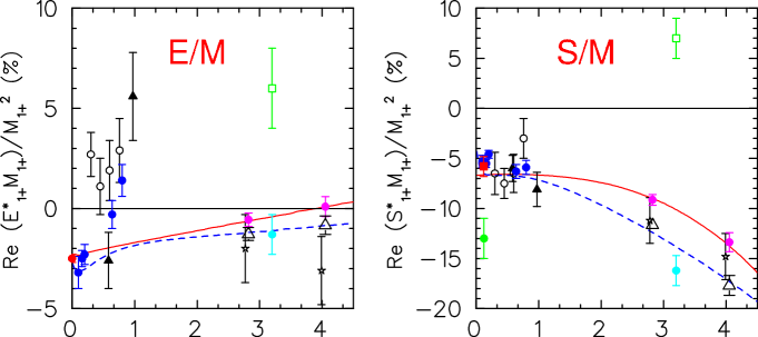
Figure 3: The $Q^{2}$ dependence of the ratios $R_{EM}^{(p\pi^{0})}$ and $R_{SM}^{(p\pi^{0})}$ at $W=1232$ MeV. The solid and dashed curves are the MAID and dynamical model results, respectively. Experimental data at $Q^{2}=0$ from Ref. [13], data at $Q^{2}$=0.1, 0.16, 0.2, 0.64, 0.8 $GeV^{2}$ from Ref. [30] and data at $Q^{2}$=2.8 and 4.0 $GeV^{2}$ from Ref. [28] (stars). Our results at $Q^{2}$=2.8 and 4.0 $GeV^{2}$, including their error bars, are obtained from MAID ($\bullet$) and the dynamical model ($\bigtriangleup$) analyses. The points at $Q^{2}=3.2$ GeV² are obtained from DESY data [31] by Ref. [32] (squares) and MAID ($\bullet$). For other data see Ref. [33].

Table 2: Our results for the magnetic transition form factor $G_{M}^{*}$ and for the ratios $R_{EM}$ and $R_{SM}$, at $Q^{2}$=2.8 (upper row) and 4.0 (lower row) (GeV/c)², extracted from a global fit to the data with MAID and the dynamical model as discussed in the text. Results from Ref. [28] are listed for comparison. Ratios are given in (%).

ratios	$Q^{2}(GeV^{2})$	MAID	DM	Ref. [28]
$G_{M}^{*}\times 100$	2.8	$6.78\pm 0.05$	$7.00\pm 0.04$	$6.9\pm 0.4$
	4.0	$2.86\pm 0.02$	$3.04\pm 0.02$	$2.9\pm 0.2$
$R_{EM}$	2.8	$-0.56\pm 0.33$	$-1.28\pm 0.32$	$-2.00\pm 1.7$
	4.0	$0.09\pm 0.50$	$-0.84\pm 0.46$	$-3.1\pm 1.7$
$R_{SM}$	2.8	$-9.14\pm 0.54$	$-11.65\pm 0.52$	$-11.2\pm 2.3$
	4.0	$-13.37\pm 0.95$	$-17.70\pm 1.0$	$-14.8\pm 2.3$

We have also re-analyzed older DESY [31] data measured at $Q^{2}=3.2(GeV/c)^{2}$ and found significantly different results for the ratios compared to a previous analysis [32]. However, since these data also give a $G_{M}^{*}$ value $20\%$ below our fit curves in Figure 2, we did not include them in our fits of the ratios.

In a similar way we also analyzed recent Bates measurements [34] for unpolarized differential cross sections, $R_{LT}$ response function and $A_{LT}$ asymmetry for $p(e,e^{\prime}\pi^{0})p$ at $Q^{2}=0.126(GeV/c)^{2}$ and obtained the following preliminary values for the E2/M1 and C2/M1 ratios

$$R_{EM}=(-2.1\pm 0.2)\%\quad\mbox{and}\quad R_{SM}=(-6.3\pm 0.2)\%\,.$$ (20)

Finally, in a double polarization experiment at Mainz [35], measuring the recoil polarization of the proton, $p(\vec{e},e^{\prime}\vec{p})\pi^{0}$ at $Q^{2}=0.121(GeV/c)^{2}$, a preliminary value of

$$R_{SM}=(-5.8\pm 1.0)\%\,.$$ (21)

could be extracted in a rather model-independent way from the x-component of the recoil polarization $P_{x}$, which is very sensitive to the resonant $S_{1+}$ multipole.

Our extracted values for $R_{EM}$ and $R_{SM}$ and a comparison with the results of Ref. [28] are presented in Table 2 and shown in Figure 3. The main difference between our results and those of Ref. [28] is that our values of $R_{EM}$ show a clear tendency to cross zero and change sign as $Q^{2}$ increases. This is in contrast with the results obtained in the original analysis [28] of the data which concluded that $R_{EM}$ would stay negative and tend toward more negative values with increasing $Q^{2}$.

4 CONCLUSIONS

In the framework of fixed-t dispersion relations with the new and very precise data obtained at MAMI in Mainz we have obtained a new partial wave analysis for pion photoproduction. The uncertainties in most multipoles could be considerably improved compared to previous analyses. At the resonance position, where the phase passes $90^{\circ}$, we obtain an E2/M1 ratio of $R_{EM}=(-2.5\pm 0.1)\%$. At the pole in the complex plane we obtain the ratio of the resonant electric and magnetic multipoles as $R_{\Delta}=-0.035-0.046i$. This is a further model-independent ratio that can be determined in any analysis or calculation of pion photoproduction.

For pion electroproduction, we have re-analyzed the recent JLab data for electroproduction of the $\Delta(1232)$ resonance via $p(e,e^{\prime}p)\pi^{0}$ with two models for pion electroproduction, both of which give excellent descriptions of the existing data. In contrast to previous findings, our models indicate that $R_{EM}$, starting from a small and negative value at the real photon point, actually exhibits a clear tendency to cross zero and change sign as $Q^{2}$ increases. It will be most interesting to have data at yet higher momentum transfer in order to see whether such a trend continues, which would be a sign for a rather slow approach towards the pQCD region. Furthermore, the absolute value of $R_{SM}$ is strongly increasing, which indicates that the pQCD prediction of $R_{SM}\rightarrow constant$ is not yet reached.

5 ACKNOWLEDGMENTS

We wish to thank R. Beck, R. Leukel, H. Schmieden, R. Gothe and C. Papanicolas for their contribution on the experimental data. This work was supported in part by NSC under Grant No. NSC89-2112-M002-038, by Deutsche Forschungsgemeinschaft (SFB443) and by a joint project NSC/DFG TAI-113/10/0.

References

- [1] C. M. Becchi and G. Morpurgo, Phys. Lett. 17 (1965) 352.
- [2] R. Koniuk and N. Isgur, Phys. Rev. D 21 (1980) 1868.
- [3] S. S. Gershteyn and G. V. Dzhikiya, Sov. J. Nucl. Phys. 34 (1981) 870.
- [4] N. Isgur, G. Karl and R. Koniuk, Phys. Rev. D 25 (1982) 2394.
- [5] A. J. Buchmann, E. Hernandez and A. Faessler, Phys. Rev. C 55 (1997) 448.
- [6] D. Drechsel and M. M. Giannini, Phys. Lett. 143 B (1984) 329.
- [7] S. Capstick and G. Karl, Phys. Rev. D 41 (1990) 2767.
- [8] S. Capstick, Phys. Rev. D 46 (1992) 2864.
- [9] K. Bermuth, D. Drechsel, L. Tiator and J. B. Seaborn, Phys. Rev. D 37 (1988) 89.
- [10] A. Wirzba and W. Weise, Phys. Lett. B 188 (1987) 6.
- [11] D. B. Leinweber, T. Draper and R. Woloshyn, Contr. Baryons ’92, (1992) p. 29.
- [12] G. Blanpied et al., Phys. Rev. Lett. 79 (1997) 4337.
- [13] R. Beck et al., Phys. Rev. Lett. 78 (1997) 606.
- [14] S.J. Brodsky and G.P. Lepage, Phys. Rev. D 23, 1152 (1981);C.E. Carlson and J.L. Poor, Phys. Rev. D 38 (1988) 2758.
- [15] D. Schwela and R. Weizel, Z. Physik 221 (1969) 71.
- [16] W. Pfeil and D. Schwela, Nucl. Phys. B45 (1972) 379.
- [17] O. Hanstein, D. Drechsel, and L. Tiator, Nucl. Phys. A632 (1998) 561.
- [18] R. Beck et al., Phys. Rev. C 61 (2000) 035204.
- [19] R.A. Arndt, I.I. Strakovsky and R.L. Workman, Phys. Rev. C 56 (1997) 577.
- [20] R.M. Davidson and N.C. Mukhopadhyay, Phys. Rev. Lett. 79 (1997) 4509.
- [21] D.E. Groom et al., Eur. Phys. Jour. C 15 (2000) 1.
- [22] R.M. Davidson et al., Phys. Rev. C 59 (1999) 1059.
- [23] G. Höhler and A. Schulte, Newsletter 7 (1992) 94.
- [24] S.N. Yang, J. Phys. G 11 (1985) L205.
- [25] D. Drechsel, O. Hanstein, S.S. Kamalov and L. Tiator, Nucl. Phys. A645 (1999) 145; http://www.kph.uni-mainz.de/MAID.
- [26] S.S. Kamalov and S.N. Yang, Phys. Rev. Lett. 83 (1999) 4494.
- [27] R.A. Arndt, I.I. Strakovsky and R.L. Workman, Phys. Rev. C 53 (1996) 430.
- [28] V.V. Frolov et al., Phys. Rev. Lett. 82 (1999) 45.
- [29] J. M. Laget, Nucl. Phys. A481 (1988) 765.
- [30] R.W. Gothe, Prog. Part. Nucl. Phys. 44 (2000) 185.
- [31] R. Haidan, Report No. DESY-F21-79-03, 1979 (unpublished).
- [32] V. Burkert and L. Elouadrhiri, Phys. Rev. Lett. 75 (1995) 3614.
- [33] S. Kamalov, S.N. Yang, D. Drechsel, O. Hanstein, L. Tiator, nucl-th/0006068.
- [34] C. Mertz et al., nucl-ex/9902012.
- [35] H. Schmieden, Nucl. Phys. A663 (2000) 21.