Equilibration and freeze-out in an exploding system

Abstract. We use a simple gas model to study non-equilibrium aspects of the multiparticle dynamics relevant to heavy ion collisions. By performing numerical simulations for various initial conditions we identify several characteristic features of the fast dynamics occurring in implosion-explosion like processes.

Introduction. Thermodynamic equilibrium at an intermediate stage of a heavy ion collision is frequently a basic assumption in models of the colliding nuclear matter. These models range from statistical models of nuclear multifragmentation to the fluid dynamical models of the quark gluon plasma. In contrast, microscopic models of molecular dynamics type (e.g. RQMD, FMD and NMD), which are based upon constituent interactions do not have this assumption built in. Such models are appropriate for testing to what extent thermodynamic equilibrium is actually achieved.

Previously we have used the Nuclear Molecular Dynamics (NMD) model [1] to describe the collision dynamics and clusterization process in nucleonic matter. In a special study of the time evolution of a finite system of colliding particles we noticed that the phase space distance $d$ between particles in the combined coordinate and momentum space has a distinct time evolution for different groups of particles: For nucleons which form clusters, $d$ is initially large and rapidly decreasing until it stays small and rather constant from a certain time. This can be interpreted as freeze-out of the hard core scattering interaction. This interpretation was supported by the fact that for interactions with no hard core scattering the phase space distance for clusters always remained small. Averaged over all nucleons the phase space distance $d$ grows with time reflecting the overall expansion of the system.

The aim of the present paper is to study the behavior of a finite piece of exploding matter before and around freeze-out of hard core interaction. Before and at this stage, the evolution of the matter is highly dynamical, leading to characteristic space-time distributions of freeze-out and flow. Whether the dynamics actually results in thermodynamical equilibrium before freeze-out is not clear a priori. Different aspects of this problem have been studied previously within various approaches [2, 3, 4, 5]. In a previous paper [6] we employed a new variable, the pseudo entropy, to study the equilibration. In the present letter we use theoretically well-founded concepts to investigate the dynamics of the exploding matter.

Classical gas model. To this end we study the dynamical properties of a simple gas model, where the constituent particles interact like billard balls by classical Newtonian dynamics. A first application of this model of nuclear collisions was made in [7]. We consider a gas of identical classical balls of radius $r_{c}$. They perform classical non-relativistic hard-sphere elastic scatterings at the impact parameter $b\leq 2r_{c}$ with conservation of energy, momentum and angular momentum. (The balls do not have intrinsic rotation.) The initial configuration consists of $A$ such particles placed randomly within a sphere of radius $R$, rejecting configurations where particles overlap within the hard core distance. This puts a constraint on $R$ which should not be too small.

We prepare the system at certain energy and density, and let it evolve until the interactions between the constituents cease. We further impose spherical symmetry on the system. In this way we minimize specific complications of the interactions and the geometry, and we can concentrate on a few basic properties of the behavior of small shortlived systems, which we believe are of general interest for heavy ion physics.

We study the evolution of the matter in the gas ball in a simple dynamical process, which is initiated by ingoing flow of the particles (implosion). In this situation the system will first compress and then expand, thus simulating some basic features of a heavy ion collision.

The initial velocities of the particles are chosen as a superposition of thermal and collective motion. We use a spherically symmetric linear profile for the initial collective velocity field

$$\vec{v}(\vec{r})=v_{0f}\,\vec{r}/R$$ (1)

where $v_{0f}$ is a model parameter. In our simulations we fix the total energy $E=E_{fl}+E_{th}$, and vary the fraction $\eta$ of the flow energy, $\eta=E_{fl}/E$, where $E_{fl}$ and $E_{th}$ are the flow energy and the thermal energy, respectively. Because of the way in which the system is built up, these energies will fluctuate from event to event with a relative uncertainty of order $A^{-\frac{1}{2}}$.

We use conventional nuclear scales: the mass of the constituent particle is $940$ MeV, the hard core radius is $r_{c}=0.4\,-\,0.5$ fm, and the initial radius of the gas sphere is $R=1.2\,A^{1/3}$ fm. We have performed simulations with $A=50$ and $A=100$ varying the flow velocity parameter $v_{0f}$ from $-0.5$ to $0.5$ (this could be in units of the velocity of light, $c=1$, but the velocity scale is in fact arbitrary in this model), and varying $\eta$ from $0$ (thermal explosion) to $1$ (implosion).

Freeze-out. A very important characteristics of evolving matter is the scattering rate $\nu(t)$, defined as the total number of scatterings per particle per unit time. It is obvious that in an implosion $\nu(t)$ first grows and then decreases, while in a thermal explosion it decreases. In Fig. 1 shows $\nu(t)$ for the two cases. The scattering rate roughly follows the matter density, because the mean free path $\lambda$ is inversely proportional to the density $n$ ($\lambda=1/n\sigma$, $\sigma$ being the scattering cross section).

FIG. 1.: The total scattering rate for a thermal explosion (solid curve) and an implosion (dashed curve) with $v_{0f}=-0.5$. Here, and in Figs. 2 and 3 $r_{c}=0.5$ fm.

One of the most fundamental questions in heavy ion physics is when can a collection of particles be considered as coherent matter? In our simplified model we shall consider particles which collide with other particles as the matter, whereas particles which do not scatter any more are decoupled from the matter, or frozen out. Therefore we study the space-time distribution of the last scattering points (the freeze-out field), because this defines the space-time limit of the coherent matter.

Two examples of a freeze-out field are shown in Fig. 2. It is seen that the distribution is rather spread, in particular for the thermal explosion. This disagrees with the Cooper-Frye picture [8], which assumes a sharp freeze-out hypersurface. A similar conclusion was reached in [9] for microscopic simulations of relativistic heavy ion collisions.

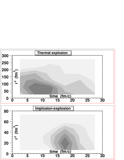
FIG. 2.: Freeze-out fields for a thermal explosion ($\eta=0$, top panel), and for an implosion ($\eta=1$, lower panel), with $100$ particles. $v_{0f}=-0.25$. We show the distribution in the $(t,r^{3})$ plane so that a uniform distribution of points in the plot corresponds to a uniform distribution in the 3 dimensional space. The distributions are based on summing the results of 10 events. In the thermal explosion, a total of $362$ last scatterings took place in the $10$ events, whereas in the implosion all particles scattered at least once in each event ($500$ scatterings in total).

An attractive way of understanding the freeze-out process is to think of the field of most recent scatterings (the scattering field): At any given time, there will be points in space where each particle had its most recent scattering. The distribution of these points in space-time is the scattering field $l(\vec{r},t;t^{\prime})$, where $\vec{r}$ and $t$ are space-time coordinates and $t^{\prime}$ is the present time (the instant at which we look at the system). The entire field $l$ as function of $\vec{r}$ and $t$ will of course change with time $t^{\prime}$, but only until complete freeze-out when the scattering field becomes fully fixed and equal to $l(\vec{r},t;\infty)$.

In addition to the freeze-out field itself, we can consider other variables defined on the freeze-out space-time coordinates. Of particular importance is the freeze-out flow field, since this may be related to the experimentally measured flow. The freeze-out flow field should be defined as a non-thermal part of the particle velocity at the freeze-out points. In general the definition of collective flow is somewhat ambiguous. However, in our case of spherical geometry it can be defined as the mean radial component of the particle velocities at the freeze-out points. In Fig. 3 we show some examples of time integrated freeze-out flow fields. Any non-zero value of these curves is a sign of collective flow.

FIG. 3.: Time integrated freeze-out flow fields for $v_{0f}=-0.25$ (the three dashed curves) and $v_{0f}=-0.5$ (the three solid curves). Within each set of curves the flow fraction $\eta$ in the initial state is varied, $\eta=0,0.5,1$ (bottom to top).

The general picture is that the freeze-out flow increases with the ingoing flow fraction $\eta$ and with the distance to the center of the explosion. Note also that even for the thermal explosion ($\eta=0$), the freeze-out flow is non-zero. One sees from the figure that within statistical errors the two families of curves reveal the scaling with the initial velocity.

Equilibration. We do not wish to make any assumptions about equilibrium, be it global or local, partial or complete. We will, however, make use of the concept of entropy, since this can formally be calculated also out of equilibrium.

To study one-body observables, we reduce the $6A$ dimensional phase-space of the $A$ particles to the one-body phase-space in $6$ dimensions in the standard way [10]. We further exploit the radial symmetry of the system by reducing the phase-space to two dimensions ($|\vec{r}|$,$|\vec{p}|$), the advantage being a gain in statistics. Then we introduce a finite grid in this reduced phase-space, dividing each of the two axes into a number of segments. But instead of working with a fixed grid in phase-space, we let the entire grid expand or contract with the majority of particles. Our experience shows that $R_{20}=(1/A\,\sum_{n=1}^{A}r_{n}^{20})^{1/20}$ is a good measure of the spatial extension of the system. This means that the physical size $\Omega_{i}$ (in units of $(2\pi\hbar)^{3}$) of cell $i$ in phase-space varies with time. We choose our grid such that all cells have equal phase space volume.

One can use the phase-space distribution of particles obtained from microscopic simulations to characterize the degree of equilibrium. First of all, for given initial conditions we perform several independent dynamical runs, and accumulate the points in different phase-space cells at each time step. In this way we obtain the occupation probability distribution $\{p_{i}\}$, where

$$p_{i}=\frac{{\mathrm{n}umber\ of\ points\ in\ box}\ i}{\mathrm{t}otal\ number\ of\ points\ in\ phase\ space}.$$ (2)

Then we repeat the simulations for a reference system where particles have sufficient time for equilibration in a fixed volume $4\pi/3R_{20}^{3}$, where $R_{20}$ is calculated from the actual spatial distribution of particles in the dynamical simulations. In this way we obtain the corresponding equilibrium distribution $\{p_{i}^{eq}\}$. We then construct the quantity

$$S=-\sum_{i}p_{i}\log(p_{i}/\Omega_{i}),$$ (3)

which in the case of equilibrium would be the real entropy [11]. Dividing by $\Omega_{i}$ inside the logarithm eliminates the trivial trend that a larger phase space cell holds more points than a smaller cell. As a measure of equilibrium we consider the quantity

$$\Sigma=\exp(S-S_{ref}).$$ (4)

$\Sigma$ is thus a measure of how close the actual phase-space distribution is to that of an equilibrized system with the same volume and energy. $\Sigma=1$ cooresponds to full equilibrium.

Since the grid expands or contracts with the particles, the information on flow is somewhat erased. One would thus expect $\Sigma$ to reach a constant value after freeze-out.

In Fig. 4 we show the behavior of the equilibrium measure $\Sigma$ in the following three cases: (a): The particles are kept inside a spherical container of radius $R=4.4$ fm until $t=20$ fm/c, when the container walls are removed; (b): $100$% ingoing flow ($\eta=1$), intended to simulate an implosion-explosion process; (c): The particles are started with $50$% thermal energy and $50$% outgoing flow ($\eta=0.5$), simulating an explosion from a not fully thermalized state.

FIG. 4.: The equilibration measure $\Sigma$ calculated for the three cases discussed in the text. The results are based on an emsemble of $20$ events with $50$ particles. Here, $r_{c}=0.4$ fm.

We notice the following features of $\Sigma$ in this figure: In the case (a) $\Sigma\simeq 1$ as long as particles are kept in the container, reflecting the fact that the system is in equilibrium. Then when the container is removed, the system goes out of equilibrium and $\Sigma$ decreases until collisions between the particles cease. This is as intuitively expected. Now, in the implosion-explosion case (b), we do not know in advance if the system will reach a state of equilibrium or not. Here, $\Sigma$ starts from a low value, since the initial state is far from equilibrium. As collisions tend to equilibrize the system, $\Sigma$ increases, but does not reach the equilibrium $\Sigma=1$. However, additional analyses show that the particles obtain a nearly Maxwellian velocity distribution from $t=6$ fm/c, which is also the time of maximum compression. During the de-equilibration time, $\Sigma$ decreases, and the rate of decrease reflects the dynamics of freeze-out. It is interesting to note that the thermal explosion (a) and the “non-thermal explosion” (c) both approach the same asymptotic value $\Sigma\simeq 0.55$, as does the implosion-explosion case. Therefore we cannot use the asymtotic behavior of $\Sigma$ to conclude about the degree of equilibrium at early stages of the system evolution. The asymptotic value of $\Sigma$ is not universal, for instance for $100$% outgoing flow $\Sigma$ is approximately constant $\simeq 0.4$.

Conclusions. We have performed dynamical simulations within a simple gas model and analysed the results both with regard to freeze-out, flow, and degree of equilibrium. The space-time distributions of last scatterings are broad in both space and time. Without using any assumptions about equilibrium we have defined the freeze-out collective flow, at least for the simple geometry adopted here. A general trend is that the freeze-out distribution is sharper and the freeze-out flow is stronger when the system goes through a state of high compression. Our calculations show that the maximum compression coincides with the maximum degree of equilibrium, but even at this stage equilibration is not complete. The present investigation uses a very schematic interaction. In the future we are planning to extend the study to other types of interaction.

Our general conclusion is that small systems evolving under fast dynamics exhibit many features which cannot be described adequately by equilibrium concepts.

Acknowledgments. This work was in part supported by the Danish Natural Science Research Council. JPB thanks the Nuclear Theory Group at GSI Darmstadt, where part of this work was done. GN thanks the Niels Bohr Institute, and and The Leon Rosenfeld Foundation and the Lørup Foundations for financial support. INM thanks The Niels Bohr Institute, and The Humbold Foundation for financial support.

REFERENCES

- [1] J.P. Bondorf, D. Idier, I.N. Mishustin, Phys. Lett. B 359 (1995) 261.
- [2] J. Randrup, Nucl. Phys. A314 (1979) 429–453.
- [3] G. Baym, Phys. Lett. 138B (1984) 18–22.
- [4] H. Heiselberg and X.-N. Wang, Phys. Rev. C 53 (1996) 1892–1902 and references herein.
- [5] J.P. Bondorf, O. Friedrichsen, D. Idier, I.N. Mishustin, Nucl. Phys. A 624 (1997) 706–737.
- [6] G. Neergaard, J.P. Bondorf, I.N. Mishustin: Thermodynamics of explosions, in the Proceedings of “Bologna 2000 – Structure of the nucleus”, nucl-th/0009009.
- [7] J.P. Bondorf, H.T. Feldmeier, S. Garpman, E.C. Halbert, Phys. Lett. B (1976) 217.
- [8] F. Cooper and G. Frye, Phys. Rev. D 10, 186 (1974).
- [9] L.V. Bravina, I.N. Mishustin, J.P. Bondorf, A. Faessler, and E.E. Zabrodin, Phys. Rev. C 60 44905 (1999).
- [10] E.H. Kennard: Kinetic Theory of Gases, McGraw-Hill, 1938.
- [11] Landau and Lifshitz: Statistical Physics I, Pergamon Press, 1968.