Abstract

The elastic backward proton-deuteron scattering is analyzed within a covariant approach based on the invariant expansion of the reaction amplitude. The relativistic invariant equations for all the polarization observables are presented. Within the impulse approximation the relation of the tensor analyzing power $T_{20}$ and the polarization transfer $\kappa_{0}$ to $P$-wave components of the deuteron wave function is found. The comparison of the theoretical calculations with experimental data is presented. An experimental verification of the reaction mechanism is suggested by constructing some combinations of different observables.

As known, the study of polarization phenomena in hadron and hadron-nucleus collisions gives more detailed information about dynamics of their interaction and the structure of colliding particles. Among the simplest reactions with hadron probes are processes of forward or backward scattering of protons off the deuteron. In particular the tensor analyzing power $T_{20}$ by backward $pD$ elastic scattering has been measured in Saclay yet fifteen years ago [1]. These interesting data yet can’t be understood theoretically especially at the kinetic energy of protons emitted backward $T_{p}>0.6$ GeV. The intensive experimental study of the elastic and inelastic $pD$ reaction has been continued in Dubna and Saclay (see for instance [2, 3]) and is also planed to be investigated in the nearest future at COSY [4]. All these data can’t be described within the impulse approximation by using the usual deuteron wave function having only $S$- and $D$-waves as it is shown in [5].

In this paper we concentrate our attention on the study of the contribution of a possible $P$-wave component in the deuteron wave function (DWF) by using helicity amplitudes formalism to all the polarization observables and in particular such as the tensor analyzing power $T_{20}$ and deuteron-proton polarization transfer $\kappa_{0}$. This contribution is investigated within the impulse approximation. We suggest an experimental test of the reaction mechanism by measuring some combinations of the polarization characteristics.

$\bullet~{}~{}$Invariant expansion of $pD\to Dp$ backward reaction amplitude
Let us start from the basic relativistic invariant expansion of elastic backward proton-deuteron amplitude using Itzykson-Zuber conventions [6]. (see FIG.1)

In general case the relativistic amplitude for the elastic scattering of two particles with spins $1$ and $1/2$ has $12$ relativistic invariant amplitudes, if all particles are on-mass shell and taking into account the $P$- and $T$-invariance. ($3\times 2\times 3\times 2=36$, $P$-invariance results in $18$ functions and $T$-invariance results in $12$ functions). The general form for the amplitude of reaction $pD\to Dp$ can be written in the following form:

$${\cal M}_{\sigma_{f}\sigma_{i}}^{\beta_{f}\beta_{i}}(s,t,u)~{}=~{}\left[\bar{u}_{\sigma_{f}}(p_{f})~{}{\cal Q}^{\mu\nu}(s,t,u)~{}u_{\sigma_{i}}(p_{i})\right]\xi^{*(\beta_{f})}_{\mu}(D_{f})~{}\xi^{~{}(\beta_{i})}_{\nu}(D_{i}),$$ (1)

where $u_{\sigma_{i}}(p_{i})\equiv u_{i}$ and $\bar{u}_{\sigma_{f}}(p_{f})\equiv\bar{u}_{f}$ are the spinors of the initial and final nucleons with spin projections $\sigma_{i}$ and $\sigma_{f}$ respectively; $\xi_{\mu}(D)$ is the polarization vectors of deuterons; $s,t,u$ are invariant Mandelstam’s variables

$$s=(D_{i}+p_{i})^{2}~{}~{};~{}~{}t=(D_{i}-D_{f})^{2}~{}~{};~{}~{}u=(D_{i}-p_{f})^{2}=\bar{s}~{}~{},$$ (2)

For the backward $pD\to Dp$ scattering the amplitude (1) depends only on the one kinematical variable which is chosen usually as $s$, e.g., square of the initial energy in the c.m.s. The amplitude ${\cal Q}_{\mu\nu}$ for this process contents four amplitudes and can be written in the form:

$${\cal Q}_{\mu\nu}(s)~{}=~{}{\cal Q}_{0}(s)\left(-g_{\mu\nu}+q_{\mu}q_{\nu}\right)+{\cal Q}_{1}(s)q_{\mu}q_{\nu}+{\cal Q}_{2}(s)q_{\{\mu}\gamma_{\nu\}}+i{\cal Q}_{3}(s)\gamma_{5}\varepsilon_{\mu\nu\rho\sigma}\gamma^{\rho}q^{\sigma}~{},$$ (3)

where we introduce the unit 4-vector $q=Q/\sqrt{Q^{2}},~{}Q=(D_{i}+D_{f})/2$.

$\bullet~{}~{}$ Helicity amplitudes
To calculate the observables, differential cross sections and polarization characteristics, it would be very helpful to construct the helicity amplitudes of the considered process $pD\to Dp$. Let us introduce initial (final) proton helicities $\mu_{i,f}=\pm 1/2$ and the initial (final) deuteron helicities $\lambda_{i,f}=\pm 1,0$. The number of independent helicity amplitudes is the same as the one for corresponding amplitudes incoming to ${\cal Q}^{\mu\nu}(s)$ (3) and equal to four. They can be chosen as the following

$$\Phi_{{}^{1}_{3}}={\cal M}_{+-}^{\pm\mp}=-{\cal M}_{-+}^{\mp\pm}~{};~{}~{}\Phi_{2}={\cal M}_{+-}^{00}=-{\cal M}_{-+}^{00}~{};$$ (4)

$$\Phi_{4}={\cal M}_{++}^{+0}=-{\cal M}_{++}^{0+}={\cal M}_{--}^{0-}=-{\cal M}_{--}^{-0}~{},$$ (5)

They are related to each other by using the symmetry properties:
$\bullet~{}~{}$ Parity

$${\cal M}_{-\mu_{f}-\mu_{i}}^{-\lambda_{f}-\lambda_{i}}=(-1)^{2(\mu_{i}-\lambda_{i})}{\cal M}_{\mu_{f}\mu_{i}}^{\lambda_{f}\lambda_{i}}~{};$$ (6)

$\bullet~{}~{}$ Time - reversal

$${\cal M}_{\mu_{f}\mu_{i}}^{\lambda_{f}\lambda_{i}}=(-1)^{2(\mu_{i}-\lambda_{i})}{\cal M}_{\mu_{i}\mu_{f}}^{\lambda_{i}\lambda_{f}}~{}.$$ (7)

The Eqs.(6,7) result in the following relation: ${\cal M}_{-\mu_{f}-\mu_{i}}^{-\lambda_{f}-\lambda_{i}}={\cal M}_{\mu_{i}\mu_{f}}^{\lambda_{i}\lambda_{f}}~{}.$

Using the expansion (3) for ${\cal Q}^{\mu\nu}(s)$ one can relate the relativistic invariants ${\cal Q}_{i}$ to the corresponding helicity amplitudes $\Phi_{i}$:

$$\Phi_{{}^{1}_{3}}={\varepsilon\over m}{\cal Q}_{0}\pm{\cal Q}_{3}~{};$$ (9)

$$\Phi_{2}=-{\varepsilon\over m}{\cal Q}_{0}-{p^{2}\over M^{2}}\left({\varepsilon\over m}[{\cal Q}_{0}-{\cal Q}_{1}]-2{\cal Q}_{2}\right)~{};$$ (10)

$$\Phi_{4}=-\sqrt{2}{p^{2}\over Mm}{\cal Q}_{2}-\sqrt{2}{\varepsilon\varepsilon_{D}\over Mm}{\cal Q}_{3}~{}.$$ (11)

And these helicity amplitudes can be related to the corresponding Pauli’s amplitudes $g_{i}$:

$$\Phi_{{}^{1}_{3}}=g_{1}\mp g_{4}~{};~{}~{}\Phi_{2}=-g_{2}~{};~{}~{}\Phi_{4}=\sqrt{2}g_{3}~{}.$$ (12)

$\bullet~{}~{}$ Polarization observables
Having the helicity amplitudes given by Eq.(5) one may define various polarization characteristics for the discussed process. Applying the notations used in Refs. [7, 8] we define the set of all the possible polarization observables as the following:

$$\left(\alpha;\mu|\beta;\nu\right)={Tr\left[\sigma_{\alpha}{\cal O}_{\mu}{\cal M}^{+}\sigma_{\beta}{\cal O}_{\nu}{\cal M}\right]\over Tr\left[{\cal M}^{+}{\cal M}\right]}~{},$$ (13)

with a normalization $\left(0;0|0;0\right)=1$. The subscripts $\alpha$ and $\mu$ ($\beta$ and $\nu$) refer to the polarization characteristics of the initial (final) proton and deuteron respectively; $\sigma_{\alpha}$ is the Pauli matrix, and ${\cal O}_{\mu}$ stands for a set of $3\times 3$ operators defining the deuteron polarization. The quantity $\Sigma=Tr\left[{\cal M}^{+}{\cal M}\right]$

$$\Sigma=\sum_{\text{all}{\hskip 1.42271pt}\mu,\lambda}|{\cal M}_{\mu_{f}\mu_{i}}^{\lambda_{f}\lambda_{i}}(W)|^{2}=2(|\Phi_{1}|^{2}+|\Phi_{2}|^{2}+|\Phi_{3}|^{2}+2|\Phi_{4}|^{2})$$ (14)

is related to the unpolarized differential cross section as

$${d\sigma\over d\Omega}={1\over 6}\left({m\over 4\pi\sqrt{s}}\right)^{2}\cdot\Sigma=\sigma_{0}\cdot\Sigma~{},$$ (15)

Using the time-reversal invariance one can get the relation: $\left(\alpha;\mu|\beta;\nu\right)_{\pi}=\left(\beta;\nu|\alpha;\mu\right)_{\pi}$. Another relation as the consequence from the parity invariance is $\left(\alpha;\mu|\beta;\nu\right)=0$ if $n_{L}+n_{S}$ is odd, where $n_{L,S}$ are the numbers of the indexes $L$ or $S$ appearing in the symbols $\alpha,\mu,\beta,\nu$.

As mentioned in Ref.[9], one of the goals of the future experiments is a direct reconstruction of the complex amplitudes (5). A overfull set of polarization observables for complete measurement has been proposed in Refs.[9, 10]. In terms of the helicity amplitudes this overfull set can be written as the following:

$$\left(0;NN|0;0\right)=\left(0;0|0;NN\right)=-\left[|\Phi_{1}|^{2}-2|\Phi_{2}|^{2}+|\Phi_{3}|^{2}-|\Phi_{4}|^{2}\right]\cdot\Sigma^{-1}=A_{yy}=-T_{20}/\sqrt{2}~{};$$ (17)

$$\left(0;N|0;N\right)=\left(0;S|0;S\right)=-2\left[\text{Re}\left(\Phi_{1}+\Phi_{3}\right)\Phi_{2}^{*}-|\Phi_{4}|^{2}\right]\cdot\Sigma^{-1}=D_{N}=D_{S}=A_{y}~{};$$ (18)

$$\left(0;L|0;L\right)=2\left[|\Phi_{1}|^{2}+|\Phi_{3}|^{2}\right]\cdot\Sigma^{-1}=D_{L}~{};$$ (19)

$$\left(0;LL|0;LL\right)=-2\left(0;NN|0;LL\right)=2\left[|\Phi_{1}|^{2}+4|\Phi_{2}|^{2}+|\Phi_{3}|^{2}-4|\Phi_{4}|^{2}\right]\cdot\Sigma^{-1}=D_{LL}~{};$$ (20)

$$\left(0;NN|0;NN\right)=\left[|\Phi_{1}|^{2}/2+9\text{Re}(\Phi_{1}\Phi_{3}^{*})+|\Phi_{3}|^{2}/2+2|\Phi_{2}|^{2}-2|\Phi_{4}|^{2}\right]\cdot\Sigma^{-1}=D_{NN}~{};$$ (21)

$$\left(0;NN|0;SS\right)=\left[|\Phi_{1}|^{2}/2-9\text{Re}(\Phi_{1}\Phi_{3}^{*})+|\Phi_{3}|^{2}/2+2|\Phi_{2}|^{2}-2|\Phi_{4}|^{2}\right]\cdot\Sigma^{-1}~{};$$ (22)

$$\left(0;SN|0;SN\right)=\left[\left(0;NN|0;NN\right)-\left(0;NN|0;SS\right)\right]/2=9\text{Re}(\Phi_{1}\Phi_{3}^{*})\cdot\Sigma^{-1}=D_{SN}~{};$$ (23)

$$\left(0;LN|0;LN\right)=\left(0;LS|0;LS\right)=-\left(9/2\right)\left[\text{Re}\left(\Phi_{1}+\Phi_{3}\right)\Phi_{2}^{*}+|\Phi_{4}|^{2}\right]\cdot\Sigma^{-1}=D_{LN}=D_{LS}~{};$$ (24)

$$\left(0;N|0;LS\right)=\left(0;LN|0;S\right)=-\left(0;S|0;LN\right)=-\left(0;LS|0;N\right)=3\text{Im}\left[\left(\Phi_{1}+\Phi_{3}\right)\Phi_{2}^{*}\right]\cdot\Sigma^{-1}~{};$$ (25)

$$\left(L;L|0;0\right)=\left(0;0|L;L\right)=-2\left[|\Phi_{1}|^{2}-|\Phi_{3}|^{2}+|\Phi_{4}|^{2}\right]\cdot\Sigma^{-1}=2A_{l}~{};$$ (26)

$$\left(N;N|0;0\right)=\left(0;0|N;N\right)=\left(0;0|S;S\right)=\left(S;S|0;0\right)=2\sqrt{2}\text{Re}\left[\left(\Phi_{1}-\Phi_{2}\right)\Phi_{4}^{*}\right]\cdot\Sigma^{-1}=2A_{t}~{};$$ (27)

$$\left(N;LS|0;0\right)=\left(0;0|N;LS\right)=-3\sqrt{2}\text{Im}\left[\left(\Phi_{1}+\Phi_{2}\right)\Phi_{4}^{*}\right]\cdot\Sigma^{-1}~{};$$ (28)

$$\left(0;L|L;0\right)=\left(L;0|0;L\right)=-2\left[|\Phi_{1}|^{2}-|\Phi_{3}|^{2}-|\Phi_{4}|^{2}\right]\cdot\Sigma^{-1}=-(4/3)\kappa_{l}~{};$$ (29)

$$\left(0;N|N;0\right)=\left(N;0|0;N\right)=2\sqrt{2}\text{Re}\left[\left(\Phi_{3}-\Phi_{2}\right)\Phi_{4}^{*}\right]\cdot\Sigma^{-1}=(4/3)\kappa_{t}=(2/3)\kappa_{0}~{};$$ (30)

$$\left(0;LS|N;0\right)=\left(N;0|0;LS\right)=-3\sqrt{2}\text{Im}\left[\left(\Phi_{3}+\Phi_{2}\right)\Phi_{4}^{*}\right]\cdot\Sigma^{-1}=3A_{4}~{};$$ (31)

$$\left(L;0|L;0\right)=\left[|\Phi_{1}+\Phi_{3}|^{2}+2|\Phi_{2}|^{2}-2|\Phi_{4}|^{2}\right]\cdot\Sigma^{-1}=P_{L}~{};$$ (32)

$$\left(N;0|N;0\right)=\left(S;0|S;0\right)=2\left[2\text{Re}(\Phi_{1}\Phi_{3}^{*})+|\Phi_{2}|^{2}\right]\cdot\Sigma^{-1}=P_{N}=P_{S}~{}.$$ (33)

We use a righthand coordinate system, defined in accordance with Madison convention [11]. This system is specified by a set of three orthogonal vectors $\textstyle L$, $\textstyle N$ and $\textstyle S$, where $\textstyle L$ is the unit vector along the momenta of the incident particle, $\textstyle N$ is taken to be orthogonal to $\textstyle L$, $\mathchoice{{\hbox{\boldmath$\displaystyle S$}}}{{\hbox{\boldmath$\textstyle S$}}}{{\hbox{\boldmath$\scriptstyle S$}}}{{\hbox{\boldmath$\scriptscriptstyle S$}}}=\mathchoice{{\hbox{\boldmath$\displaystyle N$}}}{{\hbox{\boldmath$\textstyle N$}}}{{\hbox{\boldmath$\scriptstyle N$}}}{{\hbox{\boldmath$\scriptscriptstyle N$}}}\times\mathchoice{{\hbox{\boldmath$\displaystyle L$}}}{{\hbox{\boldmath$\textstyle L$}}}{{\hbox{\boldmath$\scriptstyle L$}}}{{\hbox{\boldmath$\scriptscriptstyle L$}}}$.

Since the process is described by using four complex amplitudes, one needs to measure at least seven independent observables. The magnitudes of amplitudes $|\Phi_{i}|$ can be extracted from the cross section $\Sigma$, tensor analyzing power $T_{20}$, tensor-tensor spin transfer coefficient sum: $D=[(0;NN|0;NN)+(0;NN|0,SS)]$ and the spin correlation parameter $\kappa_{l}$. It has to be noted, since the observables have forms as bilinear combinations of the amplitudes, the finding of the common phase is impossible. For simplicity we put the phase of the amplitude $\Phi_{3}$ equal to zero: $\varphi_{3}=0~{}\to~{}{\text{Im}}(\Phi_{3})=0,~{}{\text{Re}}(\Phi_{3})=\sqrt{\Phi_{3}^{2}}=|\Phi_{3}|$. Then, the other phases can be obtained from the three observables: the spin transfer coefficient from the deuteron to proton, $\kappa_{0}$, and the spin correlation parameters $(N;N|0;0)$ and $(N;LS|0;0)$. These observables are mostly realistic to be measured at the moment with the existing experimental techniques [10].

$\bullet~{}~{}$ The one-nucleon exchange mechanism (ONE)
Let us consider our reaction within the framework of the impulse approximation, FIG.2. In ONE model the amplitude of the $pD\to Dp$ backward reaction has a very simple form [5]:

$${\cal Q}_{\mu\nu}^{N}=\Gamma_{\nu}{\widehat{n}-m\over m^{2}-u}\bar{\Gamma}_{\mu}~{},$$ (34)

where $\Gamma_{\nu}(\bar{\Gamma}_{\mu}=\gamma_{0}\Gamma^{+}_{\mu}\gamma_{0})$ is a deuteron vertex with one off-shell nucleon and can be written with four form factors parameterization exactly coinciding with the one used, for instance, by Gross [12, 13, 14] or Keister and Tjon [15, 16]:

$$\Psi_{\nu}={\Gamma_{\nu}(D,q)\over m^{2}-n^{2}-i0}=\varphi_{1}(u)\gamma_{\nu}+\varphi_{2}(u){n_{\nu}\over m}+\left(\varphi_{3}(u)\gamma_{\nu}+\varphi_{4}(u){n_{\nu}\over m}\right){\widehat{n}+m\over m}~{}.$$ (35)

The form factors $\varphi_{i}(u)$ are invariant scalar functions depending on the invariant $n^{2}=u$ may be computed in any reference frame. To connect this relativistic invariant formalism with the non-relativistic one we also express $\varphi_{i}$ in the deuteron rest frame in terms of partial amplitudes, namely in the $\rho$-spin classification, the two large components of the DWF $U=^{3}{\cal S}^{++}_{1}$ and $W=^{3}{\cal D}^{++}_{1}$, and the small components $V_{s}=^{1}{\cal P}^{+-}_{1}$ and $V_{t}=^{3}{\cal P}^{+-}_{1}$ as like as in [12].

By substituting Eq.(35) into Eq.(34) and making use of the identities $n=D_{i}-p_{f}=D_{f}-p_{i},~{}n^{2}=u\leq(M-m)^{2}$, after computing the quantities (3), one can find the forms of the helicity amplitudes (*) within the ONE model in terms of this positive- and negative-energy wave functions:

$$\Phi_{1}^{N}(W)=0~{};$$ (37)

$$\Phi_{2}^{N}(W)=-2\pi^{2}\left(m^{2}-u\right)\left[{\varepsilon_{D}\over M}\left(U+\sqrt{2}W\right)-2\sqrt{3}{p\over m}V_{s}\right]\left(U+\sqrt{2}W\right)-6\pi^{2}M\varepsilon_{D}V_{s}^{2}~{};$$ (38)

$$\Phi_{3}^{N}(W)=2\pi^{2}\left(m^{2}-u\right)\left[{\varepsilon_{D}\over M}\left(\sqrt{2}U-W\right)-2\sqrt{3}{p\over m}V_{t}\right]\left(\sqrt{2}U-W\right)+6\pi^{2}M\varepsilon_{D}V_{t}^{2}~{};$$ (39)

$$\Phi_{4}^{N}(W)=2\pi^{2}\left(m^{2}-u\right)\left[{\varepsilon_{D}\over M}\left(\sqrt{2}U-W\right)\left(U+\sqrt{2}W\right)\right.$$ (40)

$$\hskip 99.58464pt\left.-\sqrt{3}{p\over m}\left\{\left(\sqrt{2}U-W\right)V_{s}+\left(U+\sqrt{2}W\right)V_{t}\right\}\right]+~{}6\pi^{2}M\varepsilon_{D}V_{s}V_{t}.$$ (41)

where $P_{\text{lab}}$ is the final proton momentum. Firstly, one can see, that all the $\Phi_{i}^{N}(W)$ amplitudes are real, e.g., all the T-odd polarization correlations are equal to zero within this approximation. For example, $(N;LS|0;0)=0$. Secondly, within the ONE approximation the helicity amplitude $\Phi_{1}^{N}(W)$ is vanished because the spin-down proton in the incident channel cannot result in the spin-down deuteron in the final channel due to the lack of the spin non-flip of the proton. This leads to $(0;NN|0;NN)=(0;NN|0;SS)$. This consequence of the ONE mechanism can be verified experimentally by measuring and combining the different observables given by Eqs.(*). For example, combine the Eq.(17) and Eq.(29) one can find the helicity amplitude $\Phi_{1}(W)$: $|\Phi_{1}(W)|^{2}=(1+T_{20}/\sqrt{2}+2\kappa_{l})\cdot\Sigma/6.$

And finally, the following relation between amplitudes:

$$\Delta^{N}\equiv\Phi_{2}^{N}\Phi_{3}^{N}+(\Phi_{4}^{N})^{2}=-12\pi^{4}{M^{3}E_{\text{lab}}^{2}(2E_{\text{lab}}-M)\over m^{2}}\left[\left(\sqrt{2}U-W\right)V_{s}-\left(U+\sqrt{2}W\right)V_{t}\right]^{2}~{}$$ (42)

has a purely P-wave dependence. We have for a “Magic Circle” in the $\kappa_{0}$-$T_{20}$ plane [17] the following equation:

$${(\kappa_{0}^{N})^{2}\over 9/8}+{(T_{20}^{N}+1/(2\sqrt{2}))^{2}\over 9/8}=1-\left(4{{\Delta^{N}}\over\Sigma^{N}}\right)^{2}~{}.$$ (43)

Using general formulas for the polarization observables in terms of the $\Phi_{i}^{N}(W)$ helicity amplitudes, one can calculate all observables in terms of positive- and negative-energy wave functions, $U,W$ and $V_{s},V_{t}$ respectively. The contribution of the positive-energy wave $U,W$ to the observables is reffered to as the non-relativistic result. The parts containing the negative-energy waves $V_{s},V_{t}$ are of a purely relativistic origin and consequently they manifest genuine relativistic correction effects. Additionally there is another source for the relativistic corrections, namely so-called Lorenz boost effects coming from the transformation of the DWF from the c.m.s. to the deuteron rest frame [18].

In terms of positive-energy waves $U$ and $W$ only the helicity amplitudes have a well-known non-relativistic form. For this simple case there is the following relation: $\Delta^{N}=\Phi_{2}^{N}\Phi_{3}^{N}+(\Phi_{4}^{N})^{2}=0$. And the Lorenz boost effects do not contribute to the polarization observables.

$\bullet~{}~{}$ Results and Discussions
Let us present the calculation results for the deuteron tensor analyzing power $T_{20}$, the polarization transfer $\kappa_{0}$ and their link given by Eq.(43) obtained within the relativistic impulse approximation. In FIG’s.(3,4) $T_{20}$ and $\kappa_{0}$ for different kinds of the DWF are presented. It can be seen from these figures the inclusion of the $P$-wave to the DWF according to [13] changes the form of $T_{20}$ at $P_{lab}>0.2$ GeV/c. The shape of these observables is changed towards the experimental data by increasing the probability of $P$-wave $P_{V}$ in the DWF. The form of the polarization transfer $\kappa_{0}$ is closed to the experimental data at $P_{V}=0.4\%-0.5\%$. Although the description of the experimental data about $T_{20}$ and $\kappa_{0}$ isn’t satisfactory even by inclusion of the $P$-wave to the DWF nevertheless the $P$-wave contribution improves the description of data and shows a big sensitivity of the polarization observables presented in FIG’s.(3,4) to this effect.

The link between $T_{20}$ and $\kappa_{0}$ given by Eq.(43) is presented in FIG.5. The big sensitivity of this relation to the contribution of the $P$-wave probability $P_{V}$ is also seen from this figure. There isn’t also a satisfactory description of the experimental data nevertheless the shape of the ”Magic Circle” which is right for the conventional DWF is deformed towards the experimental data.

In principle, there is some analogy between the effects of the deuteron $P$-wave and secondary interactions contributing to the discussed observables for elastic and inelastic backward $pD$ reactions [19, 20] and [21]. The contribution of secondary interactions, in particular the triangle graphs with a pion in intermediate state, results in an improvement of the description of discussed experimental data on observables for the deuteron striping reaction $Dp\to pX$ [21].

The consequence of the ONE mechanism can be verified experimentally by measuring and combining the different observables given by Eqs,(*). For example, one can combine the Eq.(17) and Eq.(29) in order to find the helicity amplitude $\Phi_{1}^{N}(W)$. At least, one can find experimentally the kinematical region where $\Phi_{1}^{N}(W)=0$ and the ”Magic Circle” Eq.(43) can be applicable to find some information about the $P$-wave contribution to the DWF.

$~{}\bullet~{}$ Conclusions
The performed analysis has shown the following. The discussed polarization observables $T_{20}$ and $\kappa_{0}$ are very sensitive to a possible contribution of $P$-wave to the relativistic DWF. There is some analogy between the inclusion of $P$-wave to the DWF and effect of the secondary interactions which are some corrections to the ONE graph. One can propose a verification of the reaction mechanism for the elastic backward $pD$ scattering from the measuring of the polarization observable like as $\left(0;SN|0;SN\right)$ given by Eq.(23), which have to be equal zero within the relativistic ONE approximation as it is seen from Eq.(37). Any way, combining the another polarization observables which are more available for the measurement one can find experimentally whether the helicity amplitude $\Phi_{1}^{N}(W)$ is equal zero or not at some kinematical region. Therefore one can verify experimentally the validity of the relativistic invariant impulse approximation. At least, one can find some kinematical region where it is valid more less and extract some information about the $P$-wave contribution to the DWF.

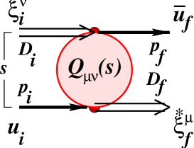
FIG. 1.: Elastic backward proton-deuteron amplitude.

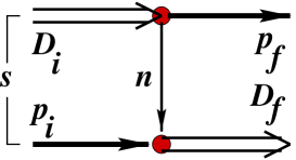
FIG. 2.: The one-nucleon exchange diagram.

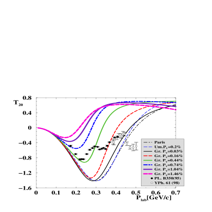
FIG. 3.: Tensor analyzing power $T_{20}$.

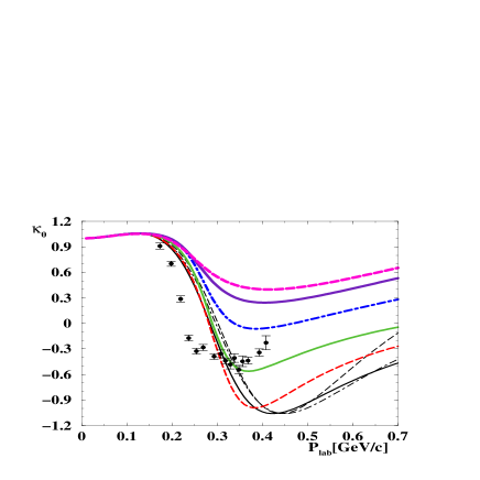
FIG. 4.: Polarization transfer coefficient $\kappa_{0}$.

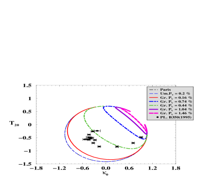
FIG. 5.: “Magic Circle” in the $\kappa_{0}$–$T_{20}$ plane.

REFERENCES

• [1] J.ย Arvieux et al., Nucl.Phys. A431 (1984) 613; Phys.Rev.Lett. 50 (1983) 19.
• [2] L.S.ย Azhgirei et al., JINR Preprint E1-94-156, Dubna, 1994; 14th Int. IUPAP Conf. on Few Body Problems in Physics (ICFBP 14), Williamsburg, VA, 26-31 May 1994; Few Body (ICFBP 14) (1994) 423; Phys.Lett. B361 (1995) 21; B391 (1997) 22.
• [3] V.ย Punjabi et al., Phys.Lett. B350 (1995) 178; S.L.ย Belostotski et al., Phys.Rev. B391 (1997) 22.
• [4] V.I.ย Komarov et al., COSY Proposal 20 โ€œExclusive deuteron break-up study with polarized protons and deuterons at COSY โ€; KFA Annual Rep. Jรผlich (1995) 64;
A.K.ย Kacharava et al., JINR Communication E1-96-42, Dubna, 1996.
• [5] A.K.ย Kerman and L.S.ย Kisslinger, Phys.Rev. 180 (1969) 1483.
• [6] C.ย Itzykson and J.B.ย  Zuber, โ€œQuantum Field Theory โ€, McGraw-Hill, 1980.
• [7] C.ย Bourrely, E.ย Leader and J.ย Soffer, Phys.Rep. 59 (1980) 95.
• [8] Ghazikhanian et al., Phys.Rev. C 43 (1991) 1532.
• [9] V.P.ย Ladygin and N.B.ย Ladygina, J.Phys.G: Nucl.Part.Phys. 23 (1997) 847.
• [10] V.P.ย Ladygin, JINR Preprint E2-96-333, Dubna, 1996.
• [11] Proceedings of the Third International Symposium on Polarization Phenomena in Nuclear Reactions. edited by H.Hย Barschall and W.ย Haeberli, (Madison) 1970.
• [12] W.W.ย Buck and F.ย Gross, Phys.Rev. D20 (1979) 2361; Phys.Lett. B63 (1976) 286.
• [13] F.ย Gross, J.W.ย VanOrden and Karlย Holinde, Phys.Rev. C45 (1992) 2094; C41 (1990) R1909.
• [14] R.G.ย Arnold, C.E.ย Carlson and F.ย Gross, Phys.Rev. C21 (1980) 1426; J.ย Hornstein and F.ย Gross, Phys.Lett. B47 (1973) 205; F.ย Gross, Phys.Rev. C26 (1982) 2203; 2226; D10 (1974) 223; 186 (1969) 1448; 140 (1965) 410B; 136 (1964) B140.
• [15] B.D.ย Keister and J.A.ย Tjon, Phys.Rev. C26 (1982) 578.
• [16] B.D.ย Keister, Phys.Rev. C24 (1981) 2628.
• [17] B.ย Kuehn, C.F.ย Perdrisat and E.A.ย Strokovsky, in: International Symposium โ€œDubna Deuteron-93โ€ (Dubna, September, 1993), unpublished; JINR, Dubna preprint E1-95-7 (1995).
• [18] L.P.ย Kaptari et al., Phys.Rev. C57 (1998) 1097.
• [19] L.A.ย Kondratyuk and F.M.ย Lev, Yad.Fiz. 26 (1977) 294.
• [20] L.A.ย Kondratyuk, F.M.ย Lev and L.V.ย Shevchenko, Preprint ITEP-120, 1980; Yad.Fiz. 33 (1981) 1208; Phys.Lett. B100 (1981) 448.
• [21] G.I.ย Lykasov, Phys.Part.Nucl. 24 (1993) 59.
Refer to caption
FIG.โ€„1.: Elastic backward proton-deuteron amplitude.
Refer to caption
FIG.โ€„2.: The one-nucleon exchange diagram.
Refer to caption
FIG.โ€„3.: Tensor analyzing power $T_{20}$.
Refer to caption
FIG.โ€„4.: Polarization transfer coefficient $\kappa_{0}$.
Refer to caption
FIG.โ€„5.: โ€œMagic Circleโ€ in the $\kappa_{0}$ $T_{20}$ plane.