The pairing Hamiltonian for one pair of nucleons bound in a potential well

M.B.Barbaro^1,2, L.Fortunato¹, A.Molinari^1,2 and M.R.Quaglia^1,2

¹ Dipartimento di Fisica Teorica dell’Università di Torino, via P.Giuria 1, I–10125, Torino, Italy
² INFN Sezione di Torino

ABSTRACT

The problem of one pair of identical nucleons sitting in ${\cal N}$ single particle levels of a potential well and interacting through the pairing force is treated introducing, in the Hamiltonian formalism, even Grassmann variables. The eigenvectors are analytically expressed solely in terms of these with coefficients fixed by the eigenvalues and the single particle energies. For these a specific model is needed: in the case of the harmonic oscillator well, for any strength of the pairing interaction, an accurate expression is derived for both the collective eigenvalue and for those trapped in between the single particle levels. Notably the latter are labelled through an index upon which they depend parabolically.

PACS:  24.10.Cn, 21.60.-n

Keywords: Grassmann algebra; Nuclear pairing interaction; Bosonization.

We have recently obtained, in the framework of the Grassmann algebra, the analytic expressions for the eigenvalues and the eigenvectors of $n$ pairs of like-nucleons interacting through the pairing Hamiltonian and sitting in one single-particle level [1].

When the single-particle levels, with angular momentum $j_{1},j_{2},\cdots j_{\cal N}$ and energies $e_{1},e_{2},\cdots e_{\cal N}$ (all the $j$’s being assumed to be different), are ${\cal N}$ usually the problem is dealt with numerically. In this case the Hamiltonian of the system reads

$$H=\sum_{\nu=1}^{\cal N}e_{\nu}\sum_{m_{\nu}=-j_{\nu}}^{j_{\nu}}\lambda^{*}_{j_{\nu}m_{\nu}}\lambda_{j_{\nu}m_{\nu}}-G\sum_{\mu,\nu=1}^{\cal N}\sum_{m_{\mu}=1/2}^{j_{\mu}}\lambda^{*}_{j_{\mu}m_{\mu}}\lambda^{*}_{j_{\mu}{\bar{m}_{\mu}}}\sum_{m_{\nu}=1/2}^{j_{\nu}}\lambda_{j_{\nu}{\bar{m}_{\nu}}}\lambda_{j_{\nu}m_{\nu}}\ ,$$

(1)

where $\lambda_{jm}$ and $\lambda^{*}_{jm}$ are the odd (anticommuting, nilpotent) Grassmann variables (associated to the nucleons annihilation and creation, respectively) and

$$\lambda_{j{\bar{m}}}\equiv(-1)^{j-m}\lambda_{j-m}\ .$$ (2)

Introducing even (commuting, nilpotent) Grassmann variables to describe a pair of fermions with vanishing third component of the total angular momentum ($M$=0), namely [2]

$$\varphi_{jm}\equiv(-1)^{j-m}\lambda_{j-m}\lambda_{jm}\ ,$$ (3)

(1) becomes

$$H=\sum_{\nu=1}^{\cal N}e_{\nu}\sum_{m_{\nu}=-j_{\nu}}^{j_{\nu}}\lambda^{*}_{j_{\nu}m_{\nu}}\lambda_{j_{\nu}m_{\nu}}-G\sum_{\mu,\nu=1}^{{\cal N}}\sum_{m_{\mu}=1/2}^{j_{\mu}}\sum_{m_{\nu}=1/2}^{j_{\nu}}\varphi^{*}_{j_{\mu}m_{\mu}}\varphi_{j_{\nu}m_{\nu}}\ .$$ (4)

In this letter we provide the eigenvectors of one pair of fermions interacting through the Hamiltonian (4) in the presence of ${\cal N}$ single particle levels in terms of (3) with coefficients expressed through the eigenvalues and the single particle energies. When the latter are those of an harmonic oscillator, an accurate, almost analytic expression is given for all the eigenvalues as well.

We start by counting the total number $N_{s}$ of states available to the system: it is given by

$$N_{s}={2\Omega\choose 2}=N_{s}^{(1)}+N_{s}^{(2)}=\frac{1}{2}\sum_{\mu\neq\nu=1}^{\cal N}2\Omega_{\mu}\cdot 2\Omega_{\nu}+\sum_{\nu=1}^{\cal N}{2\Omega_{\nu}\choose 2}$$ (5)

where

$$\Omega=\sum_{\nu=1}^{\cal N}\Omega_{\nu}=\sum_{\nu=1}^{\cal N}(j_{\nu}+1/2)\ .$$ (6)

In the above the states with the two fermions sitting on two different levels are $N_{s}^{(1)}$, those with the two fermions placed on the same level are $N_{s}^{(2)}$. Since we are interested in the physics where the pairing force is active, we consider of the $N_{s}^{(2)}$ states only the ones having the two fermions in time reversal orbits: these are $\sum_{\nu=1}^{\cal N}\Omega_{\nu}$.

Notwithstanding the presence of both the $\lambda$’s and the $\varphi$’s in (4), we search for eigenstates in the form

$$\psi=\sum_{\nu=1}^{{\cal N}}\sum_{m_{\nu}=1/2}^{j_{\nu}}\beta_{j_{\nu}m_{\nu}}\varphi^{*}_{j_{\nu}m_{\nu}}\ .$$ (7)

Using the Grassmann algebra rules, the coefficients $\beta$ are then found to obey the system of $\Omega$ equations

$$\left({\cal E}-2\varepsilon_{\nu}\right)\beta_{j_{\nu}m_{\nu}}+\sum_{{\mu}=1}^{{\cal N}}\sum_{m_{\mu}=1/2}^{j_{\mu}}\beta_{j_{\mu}m_{\mu}}=0\ ,$$ (8)

where $1\leq\nu\leq{\cal N}$, $1/2\leq m_{\nu}\leq j_{\nu}$.

We cast the above system in the $\Omega\times\Omega$ matrix form

$${\bf M}\vec{\beta}=\left(\begin{array}[]{cccccc}B_{11}&B_{12}&\cdot&\cdot&\cdot&B_{1{\cal N}}\\ B_{21}&B_{22}&\cdot&\cdot&\cdot&B_{2{\cal N}}\\ \cdot&\cdot&\cdot&\cdot&\cdot&\cdot\\ \cdot&\cdot&\cdot&\cdot&\cdot&\cdot\\ \cdot&\cdot&\cdot&\cdot&\cdot&\cdot\\ B_{{\cal N}1}&B_{{\cal N}2}&\cdot&\cdot&\cdot&B_{{\cal N}{\cal N}}\end{array}\right)\left(\begin{array}[]{c}\beta_{j_{1}1/2}\\ \beta_{j_{1}3/2}\\ \cdot\\ \cdot\\ \cdot\\ \beta_{j_{\cal N}j_{\cal N}}\end{array}\right)=0\ ,$$ (21)

where the elements of the blocks $B_{\mu\nu}$, of dimensions $\Omega_{\nu}\times\Omega_{\mu}$, are $[B_{\mu\nu}]_{\alpha\beta}=\left({\cal E}-2\varepsilon_{\nu}\right)\delta_{\mu\nu}\delta_{\alpha\beta}+1$.

In the above all the energies are expressed in units of $G$, i.e.

$$\varepsilon_{\nu}=e_{\nu}/G\ \mbox{and}\ \ {\cal E}=E/G\ .$$ (22)

The matrix ${\bf M}$ is easily diagonalized, the associated determinant being

$$\det{\bf M}=\left[\prod_{\rho=1}^{\cal N}({\cal E}-2\varepsilon_{\rho})^{\Omega_{\rho}-1}\right]\left[\prod_{\mu=1}^{\cal N}({\cal E}-2\varepsilon_{\mu})+\sum_{\nu=1}^{\cal N}\Omega_{\nu}\prod_{\mu\neq\nu=1}^{\cal N}({\cal E}-2\varepsilon_{\mu})\right]$$ (23)

and the corresponding secular equation admits $2{\cal N}$ distinct solutions. Clearly ${\cal N}$ of these are

$${\cal E}_{\rho}=2\varepsilon_{\rho}\ ,\ \mbox{with degeneracy}\ d_{\rho}=\Omega_{\rho}-1\ ,\ \ 1\leq\rho\leq{\cal N}\ ,$$ (24)

the remaining ${\cal N}$ (non-degenerate) fulfilling instead the equation [3]

$$1+f({\cal E})=0\ \ \ \mbox{with}\ \ \ f({\cal E})=\sum_{\nu=1}^{\cal N}\frac{\Omega_{\nu}}{{\cal E}-2\varepsilon_{\nu}}\ .$$ (25)

The eigenvalues (24) clearly correspond to states insensitive to the pairing interaction, being associated to a pair with non vanishing angular momentum. The solutions of (25) correspond instead to states (describing a pair coupled to an angular momentum $J=0$) affected by the pairing force.

Now, beyond the trivial solutions (24), also the eigenvalues fulfilling (25) and the associated eigenstates can be analytically obtained (at least, as we shall see, for an harmonic oscillator potential well) in a basis, of dimensions lower than (3), which generalizes the one we introduced in ref.[1].

To show how this occurs we organize, as in ref.[1], the states associated with each of the ${\cal N}$ single particle levels into two sets, embodying $\Omega_{\nu}-1$ and 1 levels, respectively (of course it must be $\Omega_{\nu}\neq 1$). Correspondingly we define the following new basis of $2{\cal N}$ normalized states $\Phi^{(a)}_{\nu}$, with $1\leq\nu\leq{\cal N}$ and $a=0,1$:

$$\left\{\begin{array}[]{cclc}\Phi^{(0)}_{\nu}&=&\frac{1}{\sqrt{d_{\nu}}}\sum_{m_{\nu}=1/2}^{j_{\nu}-1}\varphi_{j_{\nu},m_{\nu}}\ ,&\ \ \ \ \ \nu=1,\cdots{\cal N}\\ \Phi^{(1)}_{\nu}&=&\varphi_{j_{\nu},j_{\nu}}&\end{array}\ .\right.$$ (26)

In this basis the rectangular blocks $B_{\mu\nu}$ become

$$B_{\mu\nu}=\left(\begin{array}[]{cc}B^{(0)}_{\mu\nu}&{\bf a}^{T}_{\nu}\\ {\bf a}_{\mu}&B^{(1)}_{\mu\nu}\end{array}\right)\ ,$$ (29)

where the row vector ${\bf a}_{\mu}$, of dimension $(\Omega_{\mu}-1)$, is filled with ones and $B_{\mu\nu}^{(0)}$ and $B_{\mu\nu}^{(1)}$ are two matrices of dimensions $(\Omega_{\nu}-1)\times(\Omega_{\mu}-1)$ and $1\times 1$, respectively.

Then the $2{\cal N}\times 2{\cal N}$ matrix ${\bf{\cal M}}$, representing the operator ${\cal H}={\cal E}-H/G$ in the basis (26), is obtained by replacing each $B_{\mu\nu}$ with a $2\times 2$ matrix with elements given by the sum of the elements of each block in (29) (divided by the corresponding normalization factors). One thus gets

$${\bf{\cal M}}=\left(\begin{array}[]{cccccc}{\cal E}-2\varepsilon_{1}+d_{1}&\sqrt{d_{1}}&\cdot&\cdot&\sqrt{d_{1}d_{\cal N}}&\sqrt{d_{1}}\\ \sqrt{d_{1}}&{\cal E}-2\varepsilon_{1}+1&\cdot&\cdot&\sqrt{d_{\cal N}}&1\\ \cdot&\cdot&\cdot&\cdot&\cdot&\cdot\\ \cdot&\cdot&\cdot&\cdot&\cdot&\cdot\\ \sqrt{d_{\cal N}d_{1}}&\sqrt{d_{\cal N}}&\cdot&\cdot&{\cal E}-2\varepsilon_{\cal N}+d_{\cal N}&\sqrt{d_{\cal N}}\\ \sqrt{d_{1}}&1&\cdot&\cdot&\sqrt{d_{\cal N}}&{\cal E}-2\varepsilon_{\cal N}+1\end{array}\right)\ ,$$ (30)

whose determinant reads

$$\det{\bf{\cal M}} = \det\left(\begin{array}[]{cccccc}1+\frac{{\cal E}-2\varepsilon_{1}}{d_{1}}&1&\cdot&\cdot&1&1\\ 1&1+{\cal E}-2\varepsilon_{1}&\cdot&\cdot&1&1\\ \cdot&\cdot&\cdot&\cdot&\cdot&\cdot\\ \cdot&\cdot&\cdot&\cdot&\cdot&\cdot\\ 1&1&\cdot&\cdot&1+\frac{{\cal E}-2\varepsilon_{\cal N}}{d_{\cal N}}&1\\ 1&1&\cdot&\cdot&1&1+{\cal E}-2\varepsilon_{\cal N}\end{array}\right)\prod_{\nu=1}^{\cal N}d_{\nu}$$ (37)

$$= \left[\prod_{\rho=1}^{\cal N}({\cal E}-2\varepsilon_{\rho})\right]\left[\prod_{\mu=1}^{\cal N}({\cal E}-2\varepsilon_{\mu})+\sum_{\nu=1}^{\cal N}\Omega_{\nu}\prod_{\mu\neq\nu=1}^{\cal N}({\cal E}-2\varepsilon_{\mu})\right]\ .$$ (38)

From (38) both the ${\cal N}$ unperturbed solutions ${\cal E}_{\rho}=2\varepsilon_{\rho}$ and the ${\cal N}$ ones affected by the pairing interaction follow.

The latter are also obtained in the normalized basis (introduced long ago by Richardson [4] with a different technique)

$$\widetilde{\Phi}_{\nu}=\sqrt{1-\frac{1}{\Omega_{\nu}}}\left[\Phi^{(0)}_{\nu}+\frac{1}{\sqrt{d_{\nu}}}\Phi^{(1)}_{\nu}\right]\ ,\ \ \ \ \ \ \ \ \ \nu=1,\cdots{\cal N}\ ,$$ (39)

which linearly combines the building blocks of (26). Note that the index of nilpotency of the commuting variables $\widetilde{\Phi}_{\nu}$ is $\Omega_{\nu}$: hence the (39) are “more bosonic” than the (3). Indeed they are often referred to as $s$-quasibosons ($J=0$) and lead to the following ${\cal N}$ dimensional representation of ${\cal H}$

$${\bf{\widetilde{\cal M}}}=\left(\begin{array}[]{cccccc}{\cal E}-2\varepsilon_{1}+\Omega_{1}&\sqrt{\Omega_{1}\Omega_{2}}&\cdot&\cdot&\cdot&\sqrt{\Omega_{1}\Omega_{\cal N}}\\ \sqrt{\Omega_{1}\Omega_{2}}&{\cal E}-2\varepsilon_{2}+\Omega_{2}&\cdot&\cdot&\cdot&\sqrt{\Omega_{2}\Omega_{\cal N}}\\ \cdot&\cdot&\cdot&\cdot&\cdot&\cdot\\ \cdot&\cdot&\cdot&\cdot&\cdot&\cdot\\ \cdot&\cdot&\cdot&\cdot&\cdot&\cdot\\ \sqrt{\Omega_{1}\Omega_{\cal N}}&\sqrt{\Omega_{2}\Omega_{\cal N}}&\cdot&\cdot&\cdot&{\cal E}-2\varepsilon_{\cal N}+\Omega_{\cal N}\end{array}\right)\ .$$ (40)

It is worth noticing that Richardson’s basis, being of lower dimension, only yields the so-called seniority $v=0$ solutions. In contrast, our basis (26) provides the whole spectrum (any seniority) of the pairing hamiltonian eigenvalues: in the present case, of course, the $v=2$ solutions are trivial, but when several pairs are present the $v\neq 0$ solutions are important.

In general the roots of Eq.(25) cannot be given analytically for ${\cal N}>4$. Only the lowest collective eigenvalue, when $G$ is large, turns out to be (in dimensional units)

$$E_{c}\stackrel{{\scriptstyle G\to\infty}}{{\sim}}-G\sum_{\nu=1}^{\cal N}\Omega_{\nu}=-G\Omega\$$ (41)

for any potential well.

The other ${\cal N}-1$ solutions, as is well-known, get instead “trapped” between the unperturbed energies

$$2e_{\nu-1}<E_{\nu}<2e_{\nu}\ \ \ \ \ \ \ \ \ \nu=2,\cdots{\cal N}\$$ (42)

and in the limit $G\to\infty$ are given by the zeros of $f(E/G)$ and depend upon the ${\cal N}$ single particle energies $e_{\nu}$ and their degeneracies $\Omega_{\nu}$.

Remarkably, when one degeneracy, say $\Omega_{\nu}$, becomes very large, then the “trapped” eigenvalues, for any value of $G$, coincide with the free ones, i.e.

$$\lim_{\Omega_{\nu}\to\infty}E_{\mu}=\left\{\begin{array}[]{l}2e_{\mu-1}\ \ \ \ \ \ \ \mbox{for}\ \ 2\leq\mu\leq\nu\\ 2e_{\mu}\ \ \ \ \ \ \ \mbox{for}\ \ \nu<\mu\leq{\cal N}\ ,\end{array}\right.$$

whereas the lowest collective energy tends to $-\infty$.

Concerning the eigenfunctions, those (normalized) corresponding to the eigenvalues ${\cal E}_{\nu}=2\varepsilon_{\nu}$ $(\nu=1,\cdots{\cal N})$ (seniority $v=2$ states) in the basis (26) are

$$\psi_{\nu,v=2}(\Phi^{*})=\sqrt{1-\frac{1}{\Omega_{\nu}}}\left\{\left[\Phi_{\nu}^{(1)}\right]^{*}-\frac{1}{\sqrt{d_{\nu}}}\left[\Phi_{\nu}^{(0)}\right]^{*}\right\}$$ (43)

and describe a free pair sitting in the level $j_{\nu}$.

The $v=0$ eigenfunctions are more conveniently expressed in the basis (39). Here they read

$$\psi_{v=0}(\widetilde{\Phi}^{*})=\sum_{\nu=1}^{\cal N}\sqrt{\Omega_{\nu}}w_{\nu}\widetilde{\Phi}^{*}_{\nu}\ ,$$ (44)

the coefficients $w_{\nu}$ fulfilling the system of equations

$$\left({\cal E}-2\varepsilon_{\nu}\right)w_{\nu}+\sum_{\mu=1}^{\cal N}\Omega_{\mu}w_{\mu}=0\ .$$ (45)

The above is easily solved and yields the noticeable formula

$$w_{\nu}=\frac{{\cal E}-2\epsilon_{\cal N}}{{\cal E}-2\epsilon_{\nu}}w_{{\cal N}}\ .$$ (46)

Since (46) entails for large ${\cal E}$

$$w_{1}=w_{2}=\cdots=w_{\cal N}\ ,$$ (47)

the collective eigenstate in the $G\rightarrow\infty$ limit corresponds to a coherent superposition of all the $s$-quasibosons reading

$$\psi_{v=0}(E_{c})\stackrel{{\scriptstyle G\to\infty}}{{\sim}}\sum_{\nu=1}^{\cal N}\sqrt{\Omega_{\nu}}\widetilde{\Phi}^{*}_{\nu}=\sum_{\nu=1}^{\cal N}\sum_{m_{\nu}=1/2}^{j_{\nu}}\varphi^{*}_{j_{\nu}m_{\nu}}\ ,$$ (48)

which is completely symmetric in the exchange of any pair of $\varphi$, thus exhibiting the same symmetry of the pairing Hamiltonian.

Also from (46) one sees that, in the limit $G\rightarrow 0$ where ${\cal E}_{\nu}\simeq 2\epsilon_{\nu}$, only one component of the basis, i.e. the $\nu$-th one, survives in the wavefunction of the “trapped” states. The same occurs when one degeneracy, say $\Omega_{\nu}$, becomes very large: as for the eigenvalues, the eigenvectors then coincide with the $\mu$-th component of the basis for $\mu>\nu$ and with the $(\mu-1)$-th component for $\mu\leq\nu$.

We now choose the harmonic oscillator potential for the single particle energies

$$e_{N}=\left(N+\frac{3}{2}\right)\hbar\omega\ \ \ \ \ \ N=0,\cdots,\infty\$$ (49)

and for the degeneracies of the states available to a pair

$$\Omega_{N}=\frac{1}{2}(N+1)(N+2)\ .$$ (50)

In this instance the secular equation (25), when the lowest ${\cal N}$ levels are considered, becomes

$$\sum_{N=0}^{{\cal N}-1}\frac{(N+1)(N+2)}{2N+3-\widetilde{E}}=\frac{1}{\widetilde{G}}\$$ (51)

where $\widetilde{G}=G/2\hbar\omega$ and the energies are measured in units of $\hbar\omega$ $(2{\widetilde{e}}_{N}=2N+3)$.

Figure 1: The figure shows the solutions $\widetilde{E}$ of Eq.(51), for ${\cal N}$=6 (upper curves) and 8 (lower curves), as functions of $\widetilde{G}$. One can see that with the harmonic oscillator well each trapped solution $\widetilde{E}_{N}$ for $\widetilde{G}>0.1$ tends approximatively to the single particle energy $2\widetilde{e}_{N}$.

In Fig.1 the numerical solutions of (51) are displayed for ${\cal N}$=6 and 8 versus $\widetilde{G}$. Remarkably, the dependence upon $\widetilde{G}$ is lost for $\widetilde{G}\geq 0.1$. Furthermore in this regime the number of trapped solutions is obviously fixed by ${\cal N}$, but their dependence upon ${\cal N}$ is quite mild.

We now conjecture the ${\cal N}$ trapped solutions of (51), which we label with the index $\bar{N}$, to depend parabolically upon the latter, namely

$$\widetilde{E}_{\bar{N}}=a{\bar{N}}^{2}+b{\bar{N}}+c\ \ \ \ \ \ \ \ \ \ \ \ \ \ {\bar{N}}=0,\cdots{\cal N}-2$$ (52)

(the collective solution $\widetilde{E}_{c}$ will be separately treated).

To fix the coefficients $a$, $b$ and $c$, we recast (51) in the polynomial form

$$\widetilde{E}^{\cal N}+a_{1}\widetilde{E}^{{\cal N}-1}+a_{2}\widetilde{E}^{{\cal N}-2}+\cdots a_{{\cal N}-1}\widetilde{E}+a_{\cal N}=0$$ (53)

and compute the first three coefficients. They turn out to be

$$a_{1} = \frac{1}{3}{\cal N}({\cal N}+2)[\widetilde{G}({\cal N}+1)-3]$$ (54)

$$a_{2} = \frac{1}{6}{\cal N}({\cal N}-1)[-\widetilde{G}({\cal N}+1)({\cal N}+2)(2{\cal N}+3)+3{\cal N}^{2}+11{\cal N}+11]$$ (55)

$$a_{3} = \frac{1}{90}{\cal N}({\cal N}-1)({\cal N}^{2}-4)[\widetilde{G}({\cal N}+1)(15{\cal N}^{2}+40{\cal N}+27)-15({\cal N}^{2}+3{\cal N}+3)]\ .$$

Then the first three Viete equations, namely

$$\sum_{\bar{N}=0}^{{\cal N}-2}\widetilde{E}_{\bar{N}} = -a_{1}-\widetilde{E}_{c}$$ (57)

$$\sum_{\bar{N}=0}^{{\cal N}-2}\widetilde{E}^{2}_{\bar{N}} = a_{1}^{2}-2a_{2}-\widetilde{E}_{c}^{2}$$ (58)

$$\sum_{\bar{N}=0}^{{\cal N}-2}\widetilde{E}^{3}_{\bar{N}} = -3a_{3}-a_{1}(a_{1}^{2}-3a_{2})-\widetilde{E}_{c}^{3}\ ,$$ (59)

yield a non-linear system in the unknowns $a$, $b$ and $c$, if $\widetilde{E}_{c}$ is known. This system can be solved by expressing, via eq.(57), $c$ as a function of $a$ and $b$

$$c(a,b) = -\frac{1}{{\cal N}-1}\left\{\widetilde{E}_{c}+\frac{b}{2}({\cal N}-1)({\cal N}-2)+\frac{a}{6}({\cal N}-1)({\cal N}-2)(2{\cal N}-3)\right.$$ (60)

$$+ \left.\frac{1}{3}{\cal N}({\cal N}+2)\left[{\widetilde{G}}({\cal N}+1)-3\right]\right\}\ .$$

In turn (60), inserted into (58), yields $b$ as a function of $a$. One finds

$$b(a)=-\frac{15a({\cal N}^{4}-6{\cal N}^{3}+13{\cal N}^{2}-12{\cal N}+4)\pm\sqrt{\Delta}}{15({\cal N}-1)^{2}({\cal N}-2)}$$ (61)

with

$$\Delta = -15({\cal N}-1)^{2}({\cal N}-2)\left\{a^{2}({\cal N}-1)^{2}({\cal N}-1)({\cal N}-2)({\cal N}-3)\right.$$

$$+ 20\left[9\widetilde{E}_{c}^{2}+6\widetilde{E}_{c}({\cal N}+2)(\widetilde{G}{\cal N}+\widetilde{G}-3)-3({\cal N}^{3}-4{\cal N}^{2}-13{\cal N}-11)\right.$$

$$- \left.\left.\widetilde{G}^{2}{\cal N}({\cal N}-2)({\cal N}+1)^{2}({\cal N}+2)^{2}+3\widetilde{G}({\cal N}+1)({\cal N}+2)({\cal N}^{2}-4{\cal N}-3)\right]\right\}\ .$$

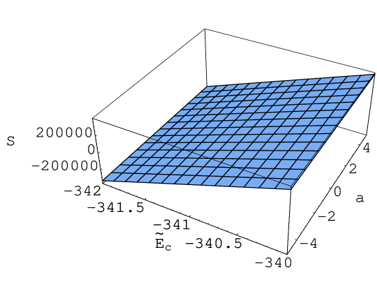
Figure 2: The figure shows the surface $S(a,\widetilde{E}_{c})$ for $-342<\widetilde{E}_{c}<-340$ and $-5<a<5$. Here the number of levels is ${\cal N}=5$ and the pairing coupling constant is $\widetilde{G}=5$.

Finally, from (59), an equation for $a$ follows, not reported here, being quite cumbersome. While we have analytically solved (57) and (58) (they are of first and second degree in $c$ and $b$, respectively), the non linear equation (59) for $a$ can only be solved numerically. Note that in (61) the plus sign in front of the square root should be taken: however both options, when inserted in (59), lead to the same equation for $a$.

It should be stressed that, because of the high degree of non-linearity of the latter, its solutions, when $\widetilde{G}$ is large, turn out to be extremely sensitive to the collective energy $\widetilde{E}_{c}$. To illustrate this issue we display in Fig.2, for ${\cal N}=5$ and $\widetilde{G}=5$, the surface (see (59))

$$S(a,\widetilde{E}_{c})=\sum_{\bar{N}=0}^{{\cal N}-2}\widetilde{E}^{3}_{\bar{N}}+3a_{3}+a_{1}(a_{1}^{2}-3a_{2})+\widetilde{E}_{c}^{3}\$$ (63)

whose zeros clearly give the values of the parameter $a$ entering into (52). It appears from the figure that even a tiny variation of $\widetilde{E}_{c}$ induces a gigantic variation in $S$, implying that $\widetilde{E}_{c}$ should be fixed with extreme precision in order to obtain the correct results for $a$, $b$ and $c$.

Now a very good expression for the collective energy, obtained by expanding Eq.(51) in the parameter $(2N+3)/\widetilde{E}$ and retaining the leading order, reads

$$\widetilde{E}_{c}^{(0)}=-\frac{\widetilde{G}}{3}{\cal N}({\cal N}+1)({\cal N}+2)+\frac{3}{2}({\cal N}+1)\ .$$ (64)

	$\widetilde{G}=1$			$\widetilde{G}=5$
${\cal N}$	$\widetilde{E}_{c}^{(e)}$	$\widetilde{E}_{c}^{(0)}$	$\widetilde{E}_{c}^{(1)}$	$\widetilde{E}_{c}^{(e)}$	$\widetilde{E}_{c}^{(0)}$	$\widetilde{E}_{c}^{(1)}$
2	-3.6055513	-3.5	-3.6041143	-35.5192213	-35.5	-35.5192121
3	-14.096330	-14.0	-14.095861	-94.0182425	-94.	-94.0182392
4	-32.582181	-32.5	-32.582012	-192.515882	-192.5	-192.515881
5	-61.070599	-61.0	-61.070528	-341.013793	-341.	-341.013793
6	-101.56156	-101.5	-101.56152	-549.512104	-549.5	-549.512104
7	-156.05444	-156.0	-156.05442	-828.010748	-828.	-828.010748
8	-226.54874	-226.5	-226.54873	-1186.50965	-1186.5	-1186.50965

Table 1: Comparison between the exact $(e)$ and the approximate $(0)$ (eq.(64)) and $(1)$ (eq.(67)) collective energies for some values of ${\cal N}$ and $\widetilde{G}$=1 and 5.

Table 1 demonstrates the validity of (64). Yet, its level of precision is not sufficient to allow a reliable determination, through (59), of $a$, because of the dramatic non-linearity displayed in Fig.2. We are thus forced to improve upon (64). To this purpose we insert into (51) the following expression for the collective energy

$$\widetilde{E}_{c}=\widetilde{E}_{c}^{(0)}+\delta$$ (65)

and again expand in the very small parameter $\delta/M(N)$ where

$$M(N)=2N+3-\widetilde{E}_{c}^{(0)}\ .$$ (66)

We thus obtain, in lieu of (64), the expression

$$\widetilde{E}_{c}^{(1)} = \widetilde{E}_{c}^{(0)}+\left[\frac{1}{\widetilde{G}}-\sum_{N=0}^{{\cal N}-1}\frac{(N+1)(N+2)}{2N+3-\widetilde{E}_{c}^{(0)}}\right]\left[\sum_{N=0}^{{\cal N}-1}\frac{(N+1)(N+2)}{{\left(2N+3-\widetilde{E}_{c}^{(0)}\right)}^{2}}\right]^{-1}$$ (67)

$$= \widetilde{E}_{c}^{(0)}-\frac{{\cal L}({\cal N},\widetilde{E}_{c}^{(0)})+2{\cal N}\left(\widetilde{E}_{c}^{(0)}+{\cal N}+2\right)-8/\widetilde{G}}{2{\cal N}+\frac{\partial{\cal L}({\cal N},\widetilde{E}_{c}^{(0)})}{\partial\widetilde{E}_{c}^{(0)}}}\ ,$$

where

$${\cal L}({\cal N},\widetilde{E}_{c}^{(0)})\equiv\left[{\left(\widetilde{E}_{c}^{(0)}\right)}^{2}-1\right]\left[\Psi\left({\cal N}+\frac{3-\widetilde{E}_{c}^{(0)}}{2}\right)-\Psi\left(\frac{3-\widetilde{E}_{c}^{(0)}}{2}\right)\right]$$ (68)

($\Psi$ being the Digamma function). Eq.(67) provides the exact collective energy, for all practical purposes, as shown in the fourth and last column of Table 1.

However, for weaker $\widetilde{G}$, (67) becomes less accurate, because the expansion parameter $(2N+3)/\widetilde{E}$ is no longer small. But this occurrence is of no consequence for the trapped solutions (up to about $\widetilde{G}=1$), since a weaker $\widetilde{G}$ also means a less severe non linearity. If, however, a more accurate value for the collective energy is wished, it can be found through the recursion relation

$$\widetilde{E}_{c}^{(k+1)}=\widetilde{E}_{c}^{(k)}+\left[\frac{1}{\widetilde{G}}-\sum_{N=0}^{{\cal N}-1}\frac{(N+1)(N+2)}{2N+3-\widetilde{E}_{c}^{(k)}}\right]\left[\sum_{N=0}^{{\cal N}-1}\frac{(N+1)(N+2)}{{\left(2N+3-\widetilde{E}_{c}^{(k)}\right)}^{2}}\right]^{-1}\ ,$$ (69)

the index $k$ labelling the order of the iteration. We have numerically checked that the iterative expansion (69) converges to the exact solution for $\widetilde{G}>0.2$.

However, the physical interesting domain for the pairing problem occurs for $\widetilde{G}=0.05-0.1$, since [5]

$$G\simeq\left\{\begin{array}[]{ll}27/A\ \mbox{MeV}&\mbox{for protons}\\ 22/A\ \mbox{MeV}&\mbox{for neutrons}\end{array}\right.$$ (70)

$A$ being the nuclear mass number, and $\hbar\omega$ should correspond to the average distance between the single particle levels inside the last occupied shell, namely $\approx 0.69$ MeV in Pb and $\approx 0.74$ MeV in Sn.

Interestingly an accurate expression for the collective energy can also be given in the regime $0\leq\widetilde{G}\leq 0.2$. Indeed here of ${\widetilde{E}}_{c}(\widetilde{G},{\cal N})$ we know the value for $\widetilde{G}=0$ (namely 3) and where it vanishes, namely for

$$\widetilde{G}_{0}=\left[\sum_{N=0}^{{\cal N}-1}\frac{(N+1)(N+2)}{\left(2N+3\right)}\right]^{-1}\ .$$ (71)

	$\widetilde{G}=0.05$
${\cal N}$	$\widetilde{E}_{c}^{(0)}$	$\widetilde{E}_{c}^{(1)}$	$\widetilde{E}_{c}^{(2)}$	$\widetilde{E}_{c}^{(3)}$	$\widetilde{E}_{c}^{(4)}$	$\widetilde{E}_{c}^{(e)}$
2	2.87617	2.88394	2.88349	2.88348	2.88348	2.88348
3	2.81180	2.87628	2.86196	2.86014	2.86012	2.86012
4	2.70198	2.89185	2.84845	2.82471	2.82056	2.82046
5	2.53580	2.86975	2.80333	2.75484	2.74104	2.74028
6	2.24594	2.63571	2.54951	2.52958	2.52886	2.52886
7	1.61587	1.84837	1.83108	1.83094	1.83094	1.83094
8	.134714	.136135	.136135	.136135	.136135	.136135
	$\widetilde{G}=0.1$
${\cal N}$	$\widetilde{E}_{c}^{(0)}$	$\widetilde{E}_{c}^{(1)}$	$\widetilde{E}_{c}^{(2)}$	$\widetilde{E}_{c}^{(3)}$	$\widetilde{E}_{c}^{(4)}$	$\widetilde{E}_{c}^{(e)}$
2	2.70757	2.72972	2.72822	2.72822	2.72822	2.72822
3	2.45586	2.61626	2.58336	2.58335	2.58335	2.58335
4	1.96617	2.21918	2.18238	2.18238	2.18238	2.18238
5	0.919942	1.00125	1.00000	1.00000	1.00000	1.00000
6	-1.66966	-1.47625	-1.48025	-1.48025	-1.48025	-1.48025
7	-8.37559	-4.88888	-5.44566	-5.44568	-5.44568	-5.44568
8	-24.4931	-3.26859	-10.7011	-11.0491	-11.0546	-11.0546

Table 2: Comparison between the exact $\widetilde{E}_{c}^{(e)}$ and the approximate $\widetilde{E}_{c}^{(k)}$ [eq.(73) and eq.(69)] collective energies for some values of ${\cal N}$ and $\widetilde{G}$=0.05 and 0.1

Moreover, the value of its derivative is $-2$ in $\widetilde{G}=0$ and

$$\left.\frac{\partial\widetilde{E}_{c}}{\partial\widetilde{G}}\right|_{{\widetilde{G}}_{0}}=-\left[\sum_{N=0}^{{\cal N}-1}\frac{(N+1)(N+2)}{2N+3}\right]^{2}\left[\sum_{N=0}^{{\cal N}-1}\frac{(N+1)(N+2)}{{\left(2N+3\right)}^{2}}\right]^{-1}$$ (72)

in $\widetilde{G}={\widetilde{G}}_{0}$.

These four constraints are fulfilled by the cubic

$$\widetilde{E}_{c}^{(0)}(\widetilde{G})=3-2\widetilde{G}-\left\{9+\left[\left.\frac{\partial\widetilde{E}_{c}}{\partial\widetilde{G}}\right|_{{\widetilde{G}}_{0}}-4\right]\widetilde{G}_{0}\right\}\frac{\widetilde{G}^{2}}{\widetilde{G}_{0}^{2}}+\left\{6+\left[\left.\frac{\partial\widetilde{E}_{c}}{\partial\widetilde{G}}\right|_{{\widetilde{G}}_{0}}-2\right]\widetilde{G}_{0}\right\}\frac{\widetilde{G}^{3}}{\widetilde{G}_{0}^{3}}\ ,$$ (73)

which thus provides an excellent starting point for the evaluation of the collective energy. Proceeding indeed as done in the large $\widetilde{G}$ domain, a perturbative expansion in a parameter $\delta$ can be set up, leading again to formula (67), but with the input $\widetilde{E}_{c}^{(k)}$ now given by the k-th iteration of (73). How remarkably accurate the results we obtain are, is displayed in Table 2.

	$\widetilde{G}=0.05$		$\widetilde{G}=0.1$		$\widetilde{G}=1$		$\widetilde{G}=5$
$\bar{N}$	$\widetilde{E}_{\bar{N}}^{(e)}$	$\widetilde{E}_{\bar{N}}^{(app)}$	$\widetilde{E}_{\bar{N}}^{(e)}$	$\widetilde{E}_{\bar{N}}^{(app)}$	$\widetilde{E}_{\bar{N}}^{(e)}$	$\widetilde{E}_{\bar{N}}^{(app)}$	$\widetilde{E}_{\bar{N}}^{(e)}$	$\widetilde{E}_{\bar{N}}^{(app)}$
0	4.2872	4.2812	3.4245	3.4266	3.1583	3.1601	3.1493	3.1510
1	6.0892	6.1056	5.6302	5.6237	5.3673	5.3621	5.3524	5.3472
2	8.1171	8.1021	7.8422	7.8485	7.6136	7.6190	7.5965	7.6015
3	10.266	10.271	10.103	10.101	9.9314	9.9297	9.9157	9.9140

Table 3: Comparison between exact $(e)$ “trapped” solutions of Eq.(51) and approximate $(app)$ ones, obtained from the ansatz (52) for ${\cal N}=5$ levels. The coefficients $(a,b,c)$ of the parabola are (0.086,1.738,4.281) when $\widetilde{G}=0.05$, (0.014,2.183,3.427) when $\widetilde{G}=0.1$, (0.027,2.175,3.160) when $\widetilde{G}=1$ and (0.029,2.167,3.151) when $\widetilde{G}=5$.

With the collective energy fixed, the coefficients $a$, $b$ and $c$ can be found.

It should be reminded that, being the system of the equations (57), (58) and (59) non-linear, more than one set of solutions is generally found: however the appropriate set is easily selected, being the one yielding energies in between the single particle levels.

We quote in Table 3 our predictions for the eigenvalues of the pairing hamiltonian for one pair in the ${\cal N}=5$ case, using as input (64) when $\widetilde{G}=1$ and $\widetilde{G}=5$ and (73) when $\widetilde{G}=0.05$ and $\widetilde{G}=0.1$. These leading orders are iterated via (69) until self-consistency is reached. Our results are seen to agree with the exact ones obtained via the numerical solution of (51) to better than $0.27\%$.

In this letter, to pave the way to the problem of any number of fermions pairs, we have solved, almost analytically, the pairing problem for one pair living in any number of harmonic oscillator levels. Crucial for this achievement has been the conjecture (52), possibly related to the specific degeneracy of the harmonic oscillator single particle levels. If this is true formulas like (52) can as well hold valid for others one body potentials, providing their degeneracy is known.

References

• [1] M.B. Barbaro, A. Molinari, F. Palumbo and M.R. Quaglia, Phys. Lett. B476 (2000) 477.
• [2] M.B. Barbaro, A. Molinari and F. Palumbo, Nucl. Phys. B 487 (1997) 492.
• [3] D.J. Rowe, β€œNuclear Collective Motion”, Metuen and Co. Ltd. (1970).
• [4] R.W. Richardson and N. Sherman, Nucl. Phys. 52 (1964) 221.
• [5] A. de-Shalit and H. Feshbach, β€œTheoretical Nuclear Physics” Vol.1 β€œNuclear Structure”, John Wiley & Sons (1990).