Hypernuclear Weak Decay Puzzle

Abstract

A general shell model formalism for the nonmesonic weak decay of the hypernuclei has been developed. It involves a partial wave expansion of the emitted nucleon waves, preserves naturally the antisymmetrization between the escaping particles and the residual core, and contains as a particular case the weak $\Lambda$-core coupling formalism. The Extreme Particle-Hole Model and the Quasiparticle Tamm-Dancoff Approximation are explicitly worked out. It is shown that the nuclear structure manifests itself basically through Pauli Principle, and a very simple expression is derived for the neutron and proton induced decays rates, $\Gamma_{n}$ and $\Gamma_{p}$, which does not involve the spectroscopic factors. We use the standard strangeness-changing weak $\Lambda N\to NN$ transition potential which comprises the exchange of the complete pseudoscalar and vector meson octets ($\pi,\eta,K,\rho,\omega,K^{*}$), taking into account some important parity violating transition operators that are systematically omitted in the literature. The interplay between different mesons in the decay of ${{}^{12}_{\Lambda}C}$ is carefully analyzed. With the commonly used parametrization in the One-Meson-Exchange Model (OMEM), the calculated rate $\Gamma_{NM}=\Gamma_{n}+\Gamma_{p}$ is of the order of the free $\Lambda$ decay rate $\Gamma^{0}$($\Gamma_{NM}^{\rm th}\cong\Gamma^{0}$) and is consistent with experiments. Yet, the measurements of $\Gamma_{n/p}=\Gamma_{n}/\Gamma_{p}$ and of $\Gamma_{p}$ are not well accounted for by the theory ($\Gamma_{n/p}^{\rm th}\>\raisebox{-2.15277pt}{$\stackrel{{\scriptstyle\textstyle<}}{{\sim}}$}\>0.42;\Gamma_{p}^{\rm th}\>\raisebox{-2.15277pt}{$\stackrel{{\scriptstyle\textstyle>}}{{\sim}}$}\>0.60~{}\Gamma^{0}$). It is suggested that, unless additional degrees of freedom are incorporated, the OMEM parameters should be radically modified.

I Introduction

The free $\Lambda$ hyperon weak decay (with transition rate $\Gamma^{0}=2.50\cdot 10^{-6}$ eV) is radically modified in the nuclear environment. First, due to Pauli principle the mesonic decay rate $\Gamma_{M}\equiv\Gamma(\Lambda\rightarrow N\pi$) is strongly blocked for $A\geq 4$. Second, new nonmesonic (NM) decay channels $\Lambda N\rightarrow NN$ become open, where there are no pions in the final state. The corresponding transition rates can be stimulated either by protons, $\Gamma_{p}\equiv\Gamma(\Lambda p\rightarrow np)$, or by neutrons, $\Gamma_{n}\equiv\Gamma(\Lambda n\rightarrow nn)$. The ultimate result is that in the mass region above $A=12$ the total hypernuclear weak decay rates $\Gamma_{M}+\Gamma_{NM}$ ($\Gamma_{NM}=\Gamma_{n}+\Gamma_{p}$) are almost constant and close to $\Gamma^{0}$ [1].

Because of the practical impossibility of having stable $\Lambda$ beams, the NM decays in hypernuclei offer the best opportunity to examine the $\Delta S=-1$ nonleptonic weak interaction between hadrons. Yet, the major motivation for studying these processes stems from the inability of the present theories to account for the measurements, in spite of the huge theoretical effort that has been invested in this issue over several decades [2, 3, 4, 5, 6, 7, 8, 9, 10, 11, 12, 13, 14, 15, 16, 17, 18, 19, 20, 21, 22, 23, 24, 25, 26]. More precisely, the theoretical models reproduce fairly well the experimental values of the total width $\Gamma_{NM}$ ($\Gamma_{NM}^{\rm exp}\cong\Gamma^{0}$), but the ratio $\Gamma_{n/p}\equiv\Gamma_{n}/\Gamma_{p}$ ($0.5\leq\Gamma_{n/p}^{\rm exp}\leq 2$) remains a puzzle.

In the one meson-exchange model (OMEM), which is very often used to describe the hypernuclear $\Lambda N\rightarrow NN$ decay, it is assumed that the process is triggered via the exchange of a virtual meson. The obvious candidate is the one-pion-exchange (OPE) mechanism, and following the pioneering investigations of Adams [3] , several calculations have been done in ${}^{12}_{\Lambda}C$, yielding: $\Gamma_{NM}^{\rm(OPE)}\cong{\Gamma^{0}}$ and $\Gamma_{n/p}^{\rm(OPE)}\cong 0.1-0.2$ [10, 12, 13, 21, 24].

The importance of the $\rho$ meson in the weak decay mechanism was first discussed by McKellar and Gibson [4]. They found that, because of the sensitivity of the results to the unknown $\Lambda N\rho$ vertex, the estimates for $\Gamma_{NM}$ could vary by a factor of 2 or 3 when the potential $V_{\rho}$ was included. (See also Ref. [5].) The present-day consensus is, however, that the effect of the $\rho$-meson on both $\Gamma_{NM}$ and $\Gamma_{n/p}$ is small [10, 12, 13, 15].

Until recently there have been quite dissimilar opinions regarding the full OMEM, which encompasses all pseudoscalar mesons ($\pi,\eta,K$) and all vector mesons ($\rho,\omega,K^{*}$). In fact, while Dubach et al. [12] claimed that the inclusion of additional exchanges in the $\pi+\rho$ model plays a major role in increasing the $n/p$ ratio, Parreño, Ramos and Bennhold [13], and Sasaki, Inoue and Oka [21] argued that the overall effect of the heavier mesons on this observable was very small. However, the two latter groups have recently corrected their calculations for a mistake in including the $K$ and $K^{*}$ mesons, and so their estimates of $\Gamma_{n/p}$ have augmented quite substantially [22, 24]. Almost simultaneously, Oset, Jido and Palomar [25] have also shown that the $K$ meson contribution was essential to increase $\Gamma_{n/p}$. However, the experimental data have not been fully explained yet.

In the last few years, many other attempts have not been particularly successful either in accounting for the measured $\Gamma_{n/p}$ ratio. To mention just a few of them: 1) analysis of the two-nucleon stimulated process $\Lambda NN\rightarrow NNN$ [7, 9, 14], 2) inclusion of interaction terms that violate the isospin ${\Delta}T=1/2$ rule [16, 20], 3) description of the short range baryon-baryon interaction in terms of quark degrees of freedom [17, 21], and 4) introduction of correlated two-pion exchange potentials besides the OPE [18]. Consistent (though not sufficient) increases of the ${n/p}$ ratio were found in the last two works. (For instance, $\Gamma_{n/p}$ was boosted up to $0.36$ for the decay of ${}^{12}_{\Lambda}C$ [18].) In fact, only Jun [26] was able so far to reproduce well the $\Gamma_{NM}$, $\Gamma_{p}$ and $\Gamma_{n/p}$ data. He has employed, in addition to the OPE, an entirely phenomenological 4-baryon point interaction for short range interaction, including the ${\Delta}T=3/2$ contribution as well, and has conveniently fixed the different model coupling constants. Let us also note that after the present work had been completed, Itonaga et al. [27] have updated their studies and have performed extensive calculations of the NM decays in the mass region $4\leq A\leq 209$, which have revealed that the correlated-$2\pi$ and $1\omega$ exchange potentials significantly improve the $\Gamma_{n/p}$ ratios over the OPE results.

In the OMEM’s, a weak baryon-baryon-meson (BBM) coupling is always combined with a strong BBM coupling. The strong one is determined experimentally with some help from the SU(3) symmetry, and the involving uncertainties have been copiously discussed in the literature [28, 29, 30, 31]. It is the weak BBM couplings which could become the largest source of errors. In fact, only the weak $N\Lambda\pi$ amplitude can be taken from the experiment, at the expense of neglecting the off-mass-shell corrections. All other weak BBM couplings are derived theoretically by using $SU(3)$ and $SU(6)_{w}$ symmetries, octet dominance, current algebra, PCAC, pole dominance, etc. [6, 12, 13, 32, 33, 34, 35, 36, 37]. Assortments of such methods have been developed and employed for a long time in weak interaction physics to explain the hyperon nonleptonic decays. Specifically, to obtain the weak BBM couplings for vector mesons the $SU(6)_{w}$ symmetry is used, which is not so well established as the $SU(3)$ symmetry is. Moreover, the results derived by way of the $SU(6)_{w}$ symmetry depend on the contributions of factorizable terms $a_{V}$ and $a_{T}$, which were only very roughly estimated [12, 32, 34]. Well aware of all these limitations, McKellar and Gibson [4] have allowed for an arbitrary phase between the $\rho$ and the $\pi$ amplitudes in the $\pi+\rho$ model. The same criterion was adopted by Takeuchi, Takaki and Band$\bar{\rm o}$ [5].

We wish to restate that the OMEM transition potential is purely phenomenological and that it is not derived from a fundamental underlying form, as happens for instance in the case of electro-magnetic transitions or the semileptonic weak decays. Only the OPE model is a natural and simple extrapolation of the mesonic decay mechanism of the $\Lambda$ to the NM process: the weak BBM coupling is identical to that used in the phenomenological description of the free $\Lambda$, and the strong vertex is the one traditionally used in describing the $\pi NN$ vertex. The assumption is that this is a valid approximation, although the pion is off the mass shell. Accordingly, all modern interpretations of the NM weak decay use the OPE as the basic building block for the medium and long range part of the decay interaction. On the contrary, the full OMEM is not used very often and, in place of the one-meson $\eta,K,\cdots$ exchanges, other mechanisms are employed as refer to above. One should also keep in mind that both the strong and weak BBM couplings, as well the meson masses, can become significantly renormalized by the nuclear environment [38].

The high momentum transfer in the NM decay makes the corresponding transition amplitude very sensitive to the short range behavior of the $NN$ and $N\Lambda$ interactions. In fact, quite recently it has been pointed out that the final state interactions (FSI) have very large influence on the total and partial decay rates [24] (see also Ref. [27]). Due to the same reason one could expect that the nuclear structure effects not included in the main field (such as the RPA or pairing correlations, higher order seniority excitations in the initial and final states, etc) should not play an important role. Yet, it could be useful to understand this issue more genuinely and to get a more complete control on the nuclear structure aspect of the problem. These are the main motivations for the present work.

The only existing shell model framework for the hypernuclear decay is the one based on the weak-coupling model (WCM) between the hyperon and the $(A-1)$ core [8, 13, 18, 27]. It involves the technique of coefficients of fractional parentage, and the spectroscopic factors (SF) explicitly appear in the expressions for the transition rates. Yet, in nuclear structure calculations it is in general simpler to evaluate the transition probabilities directly from the wave functions, instead of doing it via the SF. Here we first develop a fully general shell model formalism and then we work out thoroughly the extreme particle-hole model (EPHM) and the Quasiparticle Tamm-Dancoff Approximation (QTDA) for the even-mass hypernuclei.

Owing to the above mentioned characteristics of the OMEM it might be legitimate to ask whether it is possible to account for all three data $\Gamma_{NM}$, $\Gamma_{p}$ and $\Gamma_{n/p}$ by not fully complying with the constraints imposed by the $SU(3)$, $SU(6)_{w}$ and chiral symmetries on the BBM couplings. To find out in which way should these parameters be varied we perform a multipole expansion of the transition rate in the framework of the EPHM, which unravels in an analytic way the interplay between different mesons in each multipole channel.

Attention will be given also to the parity violating potential, since there are several typographical errors in the recent papers [13, 19, 24], regarding this part of the transition potential. We will also consider some important contributions due to the vector mesons, which, although always included in the description of the nuclear parity violation [32, 44, 45, 46], have been so far neglected in all studies of the NM hypernuclear decays, except those of Dubach et al. [12, 34].

The outline of this paper is as follows: The general shell model formalism for the hypernuclear $\Lambda N\rightarrow NN$ weak decay is developed in Sec. II. The nonrelativistic approximation for the effective Hamiltonian is presented in Sec. III. The EPHM and QTDA are explained in Sec. IV, where the multipole expansion of $\Gamma_{NM}$ is also done. Numerical evaluations of the ${{}^{12}_{\Lambda}C}\rightarrow{{}^{10}C}+nn$, and ${{}^{12}_{\Lambda}C}\rightarrow{{}^{10}B}+pn$ decay rates, are carried out in Sec. V, and the conclusions are presented in Sec. VI. The formulae for the nuclear matrix elements are summarized in the Appendix.

II Transition Rate

The decay rate, of a hypernucleus (with spin $J_{I}$ and energy ${{\cal E}}_{I}$) to residual nuclei (with spins $J_{F}$ and energies ${{\cal E}}_{F}$) and two free nucleons (with total spin $S$ and energies $\epsilon_{p}$ and $\epsilon_{P}$), follows from Fermi’s Golden Rule

$$\Gamma=2\pi\sum_{SM_{S}J_{F}M_{F}}\int|\langle{\bf p}{\bf P}SM_{S};J_{F}M_{F}|V|J_{I}M_{I}\rangle|^{2}\delta(\epsilon_{p}+\epsilon_{P}+{{\cal E}}_{F}-{{\cal E}}_{I})\frac{d{\bf p}}{(2\pi)^{3}}\frac{d{\bf P}}{(2\pi)^{3}}.$$ (1)

Here, $V$ is the weak hypernuclear potential, the wave functions for the kets $|{\bf p}{\bf P}SM_{S};J_{F}M_{F}\rangle$ and $|J_{I}M_{I}\rangle$ are assumed to be antisymmetrized and normalized, and a transformation to the relative and center of mass (c.m.) momenta, ${\bf p}$ and ${\bf P}$, is already implied, i.e.,

$${\bf p}=\frac{1}{2}({\bf p}_{1}-{\bf p}_{2}),~{}~{}~{}~{}~{}{\bf P}={\bf p}_{1}+{\bf p}_{2}.$$ (2)

It is convenient to define the quantity

$${{\cal I}}(p,P) = (4\pi)^{-4}\sum_{SM_{S}J_{F}M_{F}}\int d\Omega_{p}d\Omega_{P}|\langle{\bf p}{\bf P}SM_{S};J_{F}M_{F}|V|J_{I}M_{I}\rangle|^{2},$$ (3)

and rewrite (1) as:

$$\Gamma=\frac{16M_{N}^{3}}{\pi}\int_{0}^{\Delta_{F}}d{\epsilon}\sqrt{{\epsilon}(\Delta_{F}-{\epsilon})}{{\cal I}}(p,P),$$ (4)

where $P=2\sqrt{M_{N}{\epsilon}}$, $p=\sqrt{M_{N}(\Delta-{\epsilon})}$, $\Delta_{F}={{\cal E}}_{I}-{{\cal E}}_{F}-2M_{N}$, and $M_{N}$ is the nucleon mass.

The partial wave expansion of the wave function of the non-antisymmetrized two-particle ket $|{{\bf P}{\bf p}SM_{S}})$ is then performed:

$$({{\bf r}{\bf R}s_{1}s_{2}}|{{\bf P}{\bf p}SM_{S}}) = (4\pi)^{2}\sum_{lmLM}i^{l+L}Y^{*}_{lm}(\hat{{\bf p}})Y^{*}_{LM}(\hat{{\bf P}})({{\bf r}{\bf R}s_{1}s_{2}}|{plm,PLM,SM_{S}}),$$ (5)

where

$$({{\bf r}{\bf R}s_{1}s_{2}}|{plm,PLM,SM_{S}}) = Y_{lm}(\hat{{\bf r}})Y_{LM}(\hat{{\bf R}})j_{l}(pr)j_{L}(PR)\chi_{SM_{S}}(s_{1}s_{2}),$$ (6)

describe the spherical free waves for the outgoing particles,

$${\bf r}={\bf r}_{1}-{\bf r}_{2},~{}~{}~{}~{}~{}{\bf R}=\frac{1}{2}({\bf r}_{1}+{\bf r}_{2}).$$ (7)

are the relative and c.m. coordinates, and $l$ and $L$ are the quantum numbers for the relative (${\bf l}$) and c.m. (${\bf L}$) orbital angular momenta. After performing the angular integration in (3) we obtain:

$${{\cal I}}(p,P) = \sum_{SM_{S}J_{F}M_{F}}\sum_{lmLM}|\langle plm,PLM,SM_{S};J_{F}M_{F}|V|J_{I}M_{I}\rangle|^{2},$$ (8)

which goes into

$${{\cal I}}(p,P) = \sum_{SlL\lambda JJ_{F}}|\langle pPlL\lambda SJ,J_{F};J_{I}M_{I}|V|J_{I}M_{I}\rangle|^{2}.$$ (9)

when the angular momentum couplings: ${\bf l}+{\bf L}={\mbox{\boldmath$\lambda$}}$, ${\mbox{\boldmath$\lambda$}}+{\bf S}={\bf J}$ are carried out. The quantum number $M_{I}$ is superfluous and will be omitted from now on.

The transition potential is written in the Fock space as:

$$V=\sum_{lL\lambda SJj_{N}j_{\Lambda}}{\langle pPlL\lambda SJ|V|j_{\Lambda}j_{N}J\rangle}\left(a^{\dagger}_{pl\frac{1}{2}}a^{\dagger}_{PL\frac{1}{2}}\right)_{\lambda SJ}\cdot\left(a_{\overline{j}_{N}}a_{\overline{j}_{\Lambda}}\right)_{J},$$ (10)

where, in the same way as in (1), a transformation to the relative and c.m. momenta is implied. Here, $j_{\Lambda}$ and $j_{N}$ are the single-particle shell-model states of the decaying particles, and $a_{\overline{jm}}=(-)^{j+m}a_{j-m}$ [49]. One gets

$${{\cal I}}(p,P) = \hat{J}_{I}^{-2}\sum_{SlL\lambda JJ_{F}^{\alpha}}\left|\sum_{j_{N}j_{\Lambda}}{\langle pPlL\lambda SJ|V|j_{\Lambda}j_{N}J\rangle}\langle J_{I}||\left(a_{j_{N}}^{\dagger}a_{j_{\Lambda}}^{\dagger}\right)_{J}||J_{F}^{\alpha}\rangle\right|^{2},$$ (11)

where the transition amplitudes $\langle J_{I}||\left(a_{j_{N}}^{\dagger}a_{j_{\Lambda}}^{\dagger}\right)_{J}||J_{F}\rangle$ are reduced with respect to the angular momenta, the label $\alpha$ stands for different final states with the same spin $J_{F}$, and $\hat{J}\equiv\sqrt{2J+1}$.

The effective weak hypernuclear interaction is isospin dependent, i.e.,

$$V({\bf r},s_{\Lambda}s_{N},t_{\Lambda}t_{N})=\sum_{\tau=0,1}{{\cal V}}_{\tau}({\bf r},s_{\Lambda}s_{N}){\cal T}_{\tau},~{}~{}~{}~{}~{}{\cal T}_{\tau}=\left\{\begin{array}[]{c}1\\ \mbox{\boldmath$\tau$}_{\Lambda}\cdot\mbox{\boldmath$\tau$}_{N}\end{array}\right.,$$ (12)

and therefore the nuclear matrix elements have to be evaluated in the isospin formalism. This implies that (11) goes into

$${{\cal I}}_{m_{t_{N}}}(p,P) = \hat{J}_{I}^{-2}\sum_{S\lambda lLTJJ_{F}^{\alpha}}$$ (13)

$$\times \left|\sum_{j_{N}j_{\Lambda}}{{\cal M}}(pPlL\lambda SJT;{j_{\Lambda}j_{N},m_{t_{N}}})\langle J_{I}||\left(a_{j_{N}m_{t_{N}}}^{\dagger}a_{j_{\Lambda}}^{\dagger}\right)_{J}||J_{F}^{\alpha}\rangle\right|^{2},$$ (14)

where

$${{\cal M}}(pPlL\lambda SJT;{j_{\Lambda}j_{N},m_{t_{N}}}) = \frac{1}{\sqrt{2}}[1-(-)^{l+S+T}]$$ (16)

$$\times \sum_{\tau}({pPlL\lambda SJ}|{{\cal V}}_{\tau}|{j_{\Lambda}j_{N}J})({TM_{T}}=m_{t_{\Lambda}}+m_{t_{N}}|{\cal T}_{\tau}|{m_{t_{\Lambda}}m_{t_{N}}}),$$ (17)

is the antisymmetrized nuclear matrix element, and $m_{t_{p}}={\frac{1}{2}}$ and $m_{t_{\Lambda}}\equiv m_{t_{n}}=-{\frac{1}{2}}$. It is assumed, as usual [13], that $\Lambda$ behaves as a $|{\frac{1}{2}},-{\frac{1}{2}}\rangle$ isospin state. In that way the phenomenological $\Delta T={\frac{1}{2}}$ rule is incorporated in the effective interaction. Note that in (LABEL:2.13) and (17) $m_{t_{N}}=M_{T}-m_{t_{\Lambda}}$.

To evaluate $({pPlL\lambda SJ}|{{\cal V}}_{\tau}|{j_{\Lambda}j_{N}J})$ one has to carry out the $jj-LS$ recoupling and the Moshinsky transformation [50] on the ket $|{j_{\Lambda}j_{N}J})$ to get

$$({pPlL\lambda SJ}|{{\cal V}}_{\tau}|{j_{\Lambda}j_{N}J}) = \hat{j}_{\Lambda}\hat{j}_{N}\sum_{\lambda^{\prime}S^{\prime}{\sf nlNL}}\hat{\lambda^{\prime}}\hat{S^{\prime}}\left\{\negthinspace\begin{array}[]{ccc}l_{\Lambda}&\frac{1}{2}&j_{\Lambda}\\ l_{N}&\frac{1}{2}&j_{N}\\ \lambda^{\prime}&S^{\prime}&J\end{array}\right\}$$ (21)

$$\times ({\sf nlNL}\lambda^{\prime}|n_{\Lambda}l_{\Lambda}n_{N}l_{N}\lambda^{\prime})(pPlL\lambda SJ|{{\cal V}}_{\tau}|{\sf nlNL}\lambda^{\prime}S^{\prime}J),$$ (22)

where $(\cdots|\cdots)$ are the Moshinsky brackets [50]. Here, ${\sf l}$ and ${\sf L}$ stand for the quantum numbers of the relative and c.m. orbital angular momenta in the $\Lambda N$ system. The explicit expressions for the transition potentials are given in the next section, and the formulae that are needed to evaluate the matrix elements $(pPlL\lambda SJ|{{\cal V}}_{\tau}|{\sf nlNL}\lambda^{\prime}S^{\prime}J)$ and $({TM_{T}}|{\cal T}_{\tau}|{m_{t_{\Lambda}}m_{t_{N}}})$ are summarized in the Appendix.

When the hyperon is assumed to be weakly coupled to the $A-1$ core, which implies that the interaction of $\Lambda$ with core nucleons is disregarded, one has that $|J_{I}\rangle\equiv|(J_{C}j_{\Lambda})J_{I}\rangle$, where $J_{C}$ is the spin of the core. From

$$\langle J_{I}||\left(a_{j_{N}m_{t_{N}}}^{\dagger}a_{j_{\Lambda}}^{\dagger}\right)_{J}||J_{F}\rangle = (-)^{J_{F}+J+J_{I}}\hat{J}\hat{J}_{I}\left\{\negthinspace\begin{array}[]{ccc}J_{C}&J_{I}&j_{\Lambda}\\ J&j_{N}&J_{F}\end{array}\right\}\langle J_{C}||a_{j_{N}m_{t_{N}}}^{\dagger}||J_{F}\rangle,$$ (25)

we obtain

$${{\cal I}}_{m_{t_{N}}}(p,P) = \sum_{SlL\lambda JTJ_{F}^{\alpha}}\hat{J}^{2}$$ (26)

$$\times \left|\sum_{j_{N}}{{\cal M}}(pPlL\lambda SJT;j_{\Lambda}j_{N},m_{t_{N}})\left\{\negthinspace\begin{array}[]{ccc}J_{C}&J_{I}&j_{\Lambda}\\ J&j_{N}&J_{F}\end{array}\right\}\langle J_{C}||a_{j_{N}m_{t_{N}}}^{\dagger}||J_{F}^{\alpha}\rangle\right|^{2}.$$ (29)

Occasionally it could be convenient to include the isospin coupling as well into $\langle J_{C}||a_{j_{N}m_{t_{N}}}^{\dagger}||J_{F}\rangle$, and work with the spin-isospin reduced parentage coefficients

$$\langle J_{C}T_{C}|||a_{j_{N}\frac{1}{2}}^{\dagger}|||J_{F}T_{F}\rangle = \hat{T}_{C}\frac{\langle J_{C}T_{C}M_{T_{C}}||a_{j_{N}m_{t_{N}}}^{\dagger}||J_{F}T_{F}M_{T_{F}}\rangle}{(T_{F}M_{T_{F}}\frac{1}{2}m_{t_{N}}|T_{C}M_{T_{C}})},$$ (31)

where $T_{C},M_{T_{C}}$ and $T_{F},M_{T_{F}}$ are the isospin quantum numbers of the core and residual nuclei, respectively. In this case

$${{\cal I}}_{m_{t_{N}}}(p,P) = \hat{T}_{C}^{-2}\sum_{J_{F}^{\alpha}T_{F}SlL\lambda JT}\hat{J}^{2}(T_{F}M_{T_{F}}\frac{1}{2}m_{t_{N}}|T_{C}M_{T_{C}})^{2}$$ (32)

$$\times \left|\sum_{j_{N}}{{\cal M}}(pPlL\lambda SJ;{j_{\Lambda}j_{N},m_{t_{N}}})\left\{\negthinspace\begin{array}[]{ccc}J_{C}&J_{I}&j_{\Lambda}\\ J&j_{N}&J_{F}\end{array}\right\}\langle J_{C}T_{C}|||a_{j_{N}\frac{1}{2}}^{\dagger}|||J_{F}^{\alpha}T_{F}\rangle\right|^{2}.$$ (35)

Thus, knowing the transition potential $V$ and the initial and final nuclear wave functions $|J_{I}\rangle$ and $|J_{F}\rangle$ (or $|J_{C}\rangle$ and $|J_{F}\rangle$), we can evaluate the transition rate (4), with the integrations going up to

$$\Delta_{j_{N}m_{t_{N}}}=M_{\Lambda}-M_{N}+{\epsilon}_{j_{\Lambda}}+{\epsilon}_{j_{N}m_{t_{N}}},$$ (37)

where ${\epsilon}_{j_{\Lambda}}$ and ${\epsilon}_{j_{N}m_{t_{N}}}$ are the single particle energies.

III Effective Interaction

As the reduction of the relativistic one-meson exchange t-matrix, to the nonrelativistic effective potential $V$, is in the literature [4, 6, 10, 11, 12, 13, 24, 34, 37] it will not be repeated here. For the parity conserving (PC) potential we will just list a few results that are indispensable for establishing the notation and for the final discussion. More attention will be given to the parity violating (PV) potentials. In dealing with them some tricky details appear concerning the passage from the momentum space to the coordinate space. We first illustrate the procedure for one pseudoscalar meson ($\pi$) and one vector meson ($\rho$), and afterwards we generalize the results to all six mesons.

The effective strong (S) and weak (W) Hamiltonians read

$${{\cal H}}^{S}_{NN\pi} = ig_{NN\pi}\bar{\psi}_{N}\gamma_{5}\mbox{\boldmath$\pi$}\cdot\mbox{\boldmath$\tau$}\psi_{N},$$ (38)

$${{\cal H}}^{S}_{NN\rho} = \bar{\psi}_{N}\left(g^{V}_{NN\rho}\gamma^{\mu}+ig^{T}_{NN\rho}\frac{\sigma^{\nu\mu}\partial_{\nu}}{2M}\right)\mbox{\boldmath$\rho$}_{\mu}\cdot\mbox{\boldmath$\tau$}\psi_{N},$$ (40)

$${{\cal H}}^{W}_{\Lambda N\pi} = iG_{F}m_{\pi}^{2}\bar{\psi}_{N}\left(A_{\pi}+B_{\pi}\gamma_{5}\right)\mbox{\boldmath$\pi$}\cdot\mbox{\boldmath$\tau$}\psi_{\Lambda}\left(\negthinspace\begin{array}[]{c}0\\ 1\end{array}\right),$$ (44)

$${{\cal H}}^{W}_{\Lambda N\rho} = G_{F}m_{\pi}^{2}\bar{\psi}_{N}\left(A_{\rho}\gamma^{\mu}\gamma_{5}+B^{V}_{\rho}\gamma^{\mu}+iB_{\rho}^{T}\frac{\sigma^{\nu\mu}\partial_{\nu}}{2\overline{M}}\right)\mbox{\boldmath$\rho$}_{\mu}\cdot\mbox{\boldmath$\tau$}\psi_{\Lambda}\left(\negthinspace\begin{array}[]{c}0\\ 1\end{array}\right),$$ (48)

where $G_{F}m_{\pi}^{2}$ is the weak coupling constant, $\psi_{N}$ and $\psi_{\Lambda}$ are the baryon fields, $\pi$ and $\rho$ are the meson fields, $\tau$ is the isospin operator, $M$ the nucleon mass, and $\overline{M}$ the average between the nucleon and $\Lambda$ masses. The isospin spurion $\left(\negthinspace\begin{array}[]{c}0\\ 1\end{array}\right)$ is included in order to enforce the empirical $\Delta T={\frac{1}{2}}$ rule [13].

The corresponding nonrelativistic t-matrix in the momentum space (with the hyperon $\Lambda$ being always in the first vertex) is:

$$t_{\pi}({\bf q}) = -\mbox{\boldmath$\tau$}_{\Lambda}\cdot\mbox{\boldmath$\tau$}_{N}\frac{{{\cal A}}_{\pi}(\mbox{\boldmath$\sigma$}_{N}\cdot{\bf q})+{{\cal B}}_{\pi}(\mbox{\boldmath$\sigma$}_{\Lambda}\cdot{\bf q})(\mbox{\boldmath$\sigma$}_{N}\cdot{\bf q})}{m_{\pi}^{2}+{\bf q}^{2}},$$ (49)

$$t_{\rho}({\bf q},{\bf Q}) = -\mbox{\boldmath$\tau$}_{\Lambda}\cdot\mbox{\boldmath$\tau$}_{N}\frac{i{{\cal A}}_{\rho}(\mbox{\boldmath$\sigma$}_{\Lambda}\times\mbox{\boldmath$\sigma$}_{N})\cdot{\bf q}-2{{\cal A}}^{\prime}_{\rho}\mbox{\boldmath$\sigma$}_{\Lambda}\cdot{\bf Q}+{{\cal B}}_{\rho}(\mbox{\boldmath$\sigma$}_{\Lambda}\times{\bf q})(\mbox{\boldmath$\sigma$}_{N}\times{\bf q})-{{\cal B}}^{\prime}_{\rho}}{m_{\rho}^{2}+{\bf q}^{2}},$$ (51)

where the coupling constants ${{\cal A}}_{M}$, ${{\cal A}}^{\prime}_{M}$, ${{\cal B}}_{M}$ and ${{\cal B}}^{\prime}_{M}$ are defined in Table I, and

$${\bf q} = {\bf p}^{\prime}-{\bf p};~{}~{}~{}~{}{\bf Q}=\frac{1}{2}({\bf p}^{\prime}+{\bf p}),$$ (52)

with ${\bf p}^{\prime}$ and ${\bf p}$ being, respectively, the relative momenta for the initial and final states. (We have adopted this labeling to be consistent with (2).) In the momentum space the potential reads:

$$\langle{\bf p}_{1}{\bf p}_{2}|V|{\bf p}^{\prime}_{1}{\bf p}^{\prime}_{2}\rangle = -(2\pi)^{3}\delta({\bf p}^{\prime}_{1}+{\bf p}^{\prime}_{2}-{\bf p}_{1}-{\bf p}_{2})t({\bf q},{\bf Q}),$$ (53)

and in order to arrive to the coordinate space the Fourier transform is applied:

$$\langle{\bf r}_{1}{\bf r}_{2}|V|{\bf r}^{\prime}_{1}{\bf r}^{\prime}_{2}\rangle = \int\frac{d{\bf p}^{\prime}_{1}}{(2\pi)^{3}}\frac{d{\bf p}^{\prime}_{2}}{(2\pi)^{3}}\frac{d{\bf p}_{1}}{(2\pi)^{3}}\frac{d{\bf p}_{2}}{(2\pi)^{3}}\langle{\bf p}_{1}{\bf p}_{2}|V|{\bf p}^{\prime}_{1}{\bf p}^{\prime}_{2}\rangle$$ (54)

$$\times \exp\{i[{\bf p}^{\prime}_{1}\cdot{\bf r}^{\prime}_{1}+{\bf p}^{\prime}_{2}\cdot{\bf r}^{\prime}_{2}-{\bf p}_{1}\cdot{\bf r}_{1}-{\bf p}_{2}\cdot{\bf r}_{2}]\}.$$ (56)

After some trivial integrations and the coordinate transformation:

$${\bf x} = {\bf r}-{\bf r}^{\prime};~{}~{}~{}~{}{\bf X}=\frac{1}{2}({\bf r}^{\prime}+{\bf r}),$$ (57)

we get

$$\langle{\bf r}_{1}{\bf r}_{2}|V|{\bf r}^{\prime}_{1}{\bf r}^{\prime}_{2}\rangle = -\delta({\bf R}^{\prime}-{\bf R})\int\frac{d{\bf Q}}{(2\pi)^{3}}\frac{d{\bf q}}{(2\pi)^{3}}\exp[i({\bf Q}\cdot{\bf x}+{\bf q}\cdot{\bf X})]t({\bf q},{\bf Q}).$$ (58)

To carry out the integration on ${\bf q}$ and ${\bf Q}$ we make use of the result:

$$\int\frac{d{\bf Q}}{(2\pi)^{3}}\frac{d{\bf q}}{(2\pi)^{3}}{\bf q}\frac{e^{i({\bf Q}\cdot{\bf x}+{\bf q}\cdot{\bf X})}}{m_{M}^{2}+{\bf q}^{2}}=-i\delta({\bf r}^{\prime}-{\bf r}){\bf f}_{M}^{(-)}(r),$$ (59)

(60)

$$\int\frac{d{\bf Q}}{(2\pi)^{3}}\frac{d{\bf q}}{(2\pi)^{3}}{\bf Q}\frac{e^{i({\bf Q}\cdot{\bf x}+{\bf q}\cdot{\bf X})}}{m_{M}^{2}+{\bf q}^{2}}=\frac{i}{2}\delta({\bf r}^{\prime}-{\bf r}){\bf f}_{M}^{(+)}(r),$$ (61)

$$\int\frac{d{\bf Q}}{(2\pi)^{3}}\frac{d{\bf q}}{(2\pi)^{3}}(\mbox{\boldmath$\sigma$}_{1}\cdot{\bf q})(\mbox{\boldmath$\sigma$}_{2}\cdot{\bf q})\frac{e^{i({\bf Q}\cdot{\bf x}+{\bf q}\cdot{\bf X})}}{m_{M}^{2}+{\bf q}^{2}}=-\delta({\bf r}^{\prime}-{\bf r})[f^{S}_{M}(r)(\mbox{\boldmath$\sigma$}_{1}\cdot\mbox{\boldmath$\sigma$}_{2})+f^{T}_{M}(r)S_{12}(\hat{r})],$$ (62)

(63)

$$\int\frac{d{\bf Q}}{(2\pi)^{3}}\frac{d{\bf q}}{(2\pi)^{3}}(\mbox{\boldmath$\sigma$}_{1}\times{\bf q})(\mbox{\boldmath$\sigma$}_{2}\times{\bf q})\frac{e^{i({\bf Q}\cdot{\bf x}+{\bf q}\cdot{\bf X})}}{m_{M}^{2}+{\bf q}^{2}}=-\delta({\bf r}^{\prime}-{\bf r})[2f^{S}_{M}(r)(\mbox{\boldmath$\sigma$}_{1}\cdot\mbox{\boldmath$\sigma$}_{2})-f^{T}_{M}(r)S_{12}(\hat{r})],$$ (64)

where

$$S_{12}(\hat{r}) = 3(\mbox{\boldmath$\sigma$}_{1}\cdot\hat{r})(\mbox{\boldmath$\sigma$}_{2}\cdot\hat{r})-(\mbox{\boldmath$\sigma$}_{1}\cdot\mbox{\boldmath$\sigma$}_{2})=\sqrt{\frac{24\pi}{5}}Y_{2}(\hat{r})\cdot[\mbox{\boldmath$\sigma$}_{1}\times\mbox{\boldmath$\sigma$}_{2}]_{2},$$ (66)

is the tensor operator, and the radial dependence is contained in:

$${\bf f}_{M}^{(-)}(r) = \left[\mbox{\boldmath$\nabla$},f_{M}(r)\right]=\mbox{\boldmath$\nabla$}f_{M}(r)\equiv\hat{r}\frac{\partial}{\partial r}f_{M}(r)=\hat{r}f^{\prime}_{M}(r),$$ (67)

$${\bf f}_{M}^{(+)}(r) = \left\{\mbox{\boldmath$\nabla$},f_{M}(r)\right\}=\mbox{\boldmath$\nabla$}f_{M}(r)+2f_{M}(r)\mbox{\boldmath$\nabla$},$$ (69)

$$f_{M}^{S}(r) = \frac{1}{3}\left[m_{M}^{2}f_{M}(r)-\delta({\bf r})\right],$$ (71)

$$f_{M}^{T}(r) = \frac{m_{M}^{2}}{3}\left[1+\frac{3}{m_{M}r}+\frac{3}{(m_{M}r)^{2}}\right]f_{M}(r),$$ (73)

with $\mbox{\boldmath$\nabla$}\equiv\mbox{\boldmath$\nabla$}_{12}=\mbox{\boldmath$\nabla$}_{1}=-\mbox{\boldmath$\nabla$}_{2}$, and

$$f_{M}(r) = \frac{e^{-m_{M}r}}{4\pi r};~{}~{}~{}r=|{\bf r}_{1}-{\bf r}_{2}|,$$ (74)

$$f^{\prime}_{M}(r) = -m_{M}\left(1+\frac{1}{m_{M}r}\right)f_{M}(r).$$ (76)

Thus (58) reads

$$\langle{\bf r}_{1}{\bf r}_{2}|V|{\bf r}^{\prime}_{1}{\bf r}^{\prime}_{2}\rangle = \delta({\bf r}^{\prime}-{\bf r})\delta({\bf R}^{\prime}-{\bf R})V({\bf r}),$$ (77)

where the transition potential for the $\pi+\rho$ model is:

$$V_{\pi+\rho}({\bf r}) = \mbox{\boldmath$\tau$}_{\Lambda}\cdot\mbox{\boldmath$\tau$}_{N}\left\{(\mbox{\boldmath$\sigma$}_{\Lambda}\cdot\mbox{\boldmath$\sigma$}_{N})\left[{{\cal B}}_{\pi}f_{\pi}^{S}(r)+2{{\cal B}}_{\rho}f_{\rho}^{S}(r)\right]+S_{\Lambda N}(\hat{r})\left[{{\cal B}}_{\pi}f_{\pi}^{T}(r)-{{\cal B}}_{\rho}f_{\rho}^{T}(r)\right]\right.$$ (78)

$$+ \left.{{\cal B}}^{\prime}_{\rho}f_{\rho}(r)-i{{\cal A}}_{\pi}\mbox{\boldmath$\sigma$}_{N}\cdot{\bf f}_{\pi}^{(-)}(r)-i{{\cal A}}^{\prime}_{\rho}\mbox{\boldmath$\sigma$}_{\Lambda}\cdot{\bf f}_{\rho}^{(+)}(r)+{{\cal A}}_{\rho}(\mbox{\boldmath$\sigma$}_{\Lambda}\times\mbox{\boldmath$\sigma$}_{N})\cdot{\bf f}_{\rho}^{(-)}(r)\right\}.$$ (80)

The complete potential can now be cast in the form (12), with the isoscalar ($\eta,\omega$) and isovector ($\pi,\rho$) mesons giving rise to ${{\cal V}}_{0}$ and ${{\cal V}}_{1}$, respectively, while the strange mesons ($K,K^{*}$) contribute to both. We get:

$${{\cal V}}^{PV}_{0}({\bf r},s_{1}s_{2}) = -i\mbox{\boldmath$\sigma$}_{N}\cdot\left[{{\cal A}}_{\eta}{\bf f}_{\eta}^{(-)}(r)-{{\cal A}}^{\prime}_{K^{*}_{0}}{\bf f}_{K^{*}}^{(+)}(r)\right]+i\mbox{\boldmath$\sigma$}_{\Lambda}\cdot\left[{{\cal A}}_{K_{0}}{\bf f}_{K}^{(-)}(r)-{{\cal A}}^{\prime}_{\omega}{\bf f}_{\omega}^{(+)}(r)\right]$$ (82)

$$+ (\mbox{\boldmath$\sigma$}_{\Lambda}\times\mbox{\boldmath$\sigma$}_{N})\cdot\left[{{\cal A}}_{\omega}{\bf f}_{\omega}^{(-)}(r)+{{\cal A}}_{K^{*}_{0}}{\bf f}_{K^{*}}^{(-)}(r)\right],$$ (84)

$${{\cal V}}^{PV}_{1}({\bf r},s_{1}s_{2}) = -i\mbox{\boldmath$\sigma$}_{N}\cdot[{{\cal A}}_{\pi}{\bf f}_{\pi}^{(-)}(r)-{{\cal A}}^{\prime}_{K^{*}_{1}}{\bf f}_{K^{*}}^{(+)}(r)]+i\mbox{\boldmath$\sigma$}_{\Lambda}\cdot\left[{{\cal A}}_{K_{1}}{\bf f}_{K}^{(-)}(r)-{{\cal A}}^{\prime}_{\rho}{\bf f}_{\rho}^{(+)}(r)\right]$$ (86)

$$+ (\mbox{\boldmath$\sigma$}_{\Lambda}\times\mbox{\boldmath$\sigma$}_{N})\cdot\left[{{\cal A}}_{\rho}{\bf f}_{\rho}^{(-)}(r)+{{\cal A}}_{K^{*}_{1}}{\bf f}_{K^{*}}^{(-)}(r)\right],$$ (88)

for the PV potential, and

$${{\cal V}}^{PC}_{0}({\bf r},s_{1}s_{2}) = (\mbox{\boldmath$\sigma$}_{\Lambda}\cdot\mbox{\boldmath$\sigma$}_{N})\left[{{\cal B}}_{\eta}f_{\eta}^{S}(r)+{{\cal B}}_{K_{0}}f_{K}^{S}(r)+2{{\cal B}}_{\omega}f_{\omega}^{S}(r)+2{{\cal B}}_{K^{*}_{0}}f_{K^{*}}^{S}(r)\right]$$ (89)

$$+ S_{\Lambda N}(\hat{r})\left[{{\cal B}}_{\eta}f_{\eta}^{T}(r)+{{\cal B}}_{K_{0}}f_{K}^{T}(r)-{{\cal B}}_{\omega}f_{\omega}^{T}(r)-{{\cal B}}_{K^{*}_{0}}f_{K^{*}}^{T}(r)\right]$$ (91)

$$+ {{\cal B}}^{\prime}_{\omega}f_{\omega}(r)+{{\cal B}}^{\prime}_{K^{*}_{0}}f_{K^{*}}(r),$$ (93)

$${{\cal V}}^{PC}_{1}({\bf r},s_{1}s_{2}) = (\mbox{\boldmath$\sigma$}_{\Lambda}\cdot\mbox{\boldmath$\sigma$}_{N})\left[{{\cal B}}_{\pi}f_{\pi}^{S}(r)+{{\cal B}}_{K_{1}}f_{K}^{S}(r)+2{{\cal B}}_{\rho}f_{\rho}^{S}(r)+2{{\cal B}}_{K^{*}_{1}}f_{K^{*}}^{S}(r)\right]$$ (95)

$$+ S_{\Lambda N}(\hat{r})\left[{{\cal B}}_{\pi}f_{\pi}^{T}(r)+{{\cal B}}_{K_{1}}f_{K}^{T}(r)-{{\cal B}}_{\rho}f_{\rho}^{T}(r)-{{\cal B}}_{K^{*}_{1}}f_{K^{*}}^{T}(r)\right]$$ (97)

$$+ {{\cal B}}^{\prime}_{\rho}f_{\rho}(r)+{{\cal B}}^{\prime}_{K^{*}_{1}}f_{K^{*}}(r),$$ (99)

for the PC potential. The overall coupling constants ${{\cal A}}_{M}$, ${{\cal A}}^{\prime}_{M}$, ${{\cal B}}_{M}$ and , ${{\cal B}}^{\prime}_{M}$, are listed in Table I, with the weak couplings for kaons defined as:

TABLE I.: Isoscalar ($\tau=0$) and isovector ($\tau=1$) coupling constants in units of ${G_{F}m_{\pi}^{2}}=2.21\times 10^{-7}$.

M		${{\cal A}}_{M}$	${{\cal A}}^{\prime}_{M}$	${{\cal B}}_{M}$	${{\cal B}}^{\prime}_{M}$
			$\tau=0$
$\eta$		$A_{\eta}\displaystyle\frac{g_{NN\eta}}{2M}$	$-$	$\displaystyle\frac{B_{\eta}}{2M}\displaystyle\frac{g_{NN\eta}}{2\overline{M}}$	$-$
$K$		$A_{K_{0}}\displaystyle\frac{g_{\Lambda NK}}{2M}$	$-$	$\displaystyle\frac{B_{K_{0}}}{2M}\displaystyle\frac{g_{\Lambda NK}}{2\overline{M}}$	$-$
$\omega$		$A_{\omega}\displaystyle\frac{g^{\scriptscriptstyle V}_{NN\omega}+g^{\scriptscriptstyle T}_{NN\omega}}{2M}$	$2A_{\omega}\displaystyle\frac{g^{\scriptscriptstyle V}_{NN\omega}}{2M}$	$\displaystyle\frac{B^{\scriptscriptstyle V}_{\omega}+B^{\scriptscriptstyle T}_{\omega}}{2\overline{M}}\displaystyle\frac{g^{\scriptscriptstyle V}_{NN\omega}+g^{\scriptscriptstyle T}_{NN\omega}}{2M}$	${B^{\scriptscriptstyle V}_{\omega}g^{\scriptscriptstyle V}_{NN\omega}}$
$K^{*}$		$A_{K^{*}_{0}}\displaystyle\frac{g^{\scriptscriptstyle V}_{\Lambda NK^{*}}+g^{\scriptscriptstyle T}_{\Lambda NK^{*}}}{2M}$	$2A_{K^{*}_{0}}\displaystyle\frac{g^{\scriptscriptstyle V}_{\Lambda NK^{*}}}{2M}$	$\displaystyle\frac{B^{\scriptscriptstyle V}_{K^{*}_{0}}+B^{\scriptscriptstyle T}_{K^{*}_{0}}}{2M}\frac{g^{\scriptscriptstyle V}_{\Lambda NK^{*}}+g^{\scriptscriptstyle T}_{\Lambda NK^{*}}}{2\overline{M}}$	$B^{\scriptscriptstyle V}_{K^{*}_{0}}g^{\scriptscriptstyle V}_{\Lambda NK^{*}}$
			$\tau=1$
$\pi$		$A_{\pi}\displaystyle\frac{g_{NN\pi}}{2M}$	$-$	$\displaystyle\frac{B_{\pi}}{2M}\displaystyle\frac{g_{NN\pi}}{2\overline{M}}$	$-$
$K$		$2A_{K_{1}}\displaystyle\frac{g_{\Lambda NK}}{2M}$	$-$	$\displaystyle\frac{B_{K_{1}}}{2M}\displaystyle\frac{g_{\Lambda NK}}{2\overline{M}}$	$-$
$\rho$		$A_{\rho}\displaystyle\frac{g^{\scriptscriptstyle V}_{NN\rho}+g^{\scriptscriptstyle T}_{NN\rho}}{2M}$	$2A_{\rho}\displaystyle\frac{g^{\scriptscriptstyle V}_{NN\rho}}{2M}$	$\displaystyle\frac{B^{\scriptscriptstyle V}_{\rho}+B^{\scriptscriptstyle T}_{\rho}}{2\overline{M}}\displaystyle\frac{g^{\scriptscriptstyle V}_{NN\rho}+g^{\scriptscriptstyle T}_{NN\rho}}{2M}$	${B^{\scriptscriptstyle V}_{\rho}g^{\scriptscriptstyle V}_{NN\rho}}$
$K^{*}$		$A_{K^{*}_{1}}\displaystyle\frac{g^{\scriptscriptstyle V}_{\Lambda NK^{*}}+g^{\scriptscriptstyle T}_{\Lambda NK^{*}}}{2M}$	$2A_{K^{*}_{1}}\displaystyle\frac{g^{\scriptscriptstyle V}_{\Lambda NK^{*}}}{2M}$	$\displaystyle\frac{B^{\scriptscriptstyle V}_{K^{*}_{1}}+B^{\scriptscriptstyle T}_{K^{*}_{1}}}{2M}\frac{g^{\scriptscriptstyle V}_{\Lambda NK^{*}}+g^{\scriptscriptstyle T}_{\Lambda NK^{*}}}{2\overline{M}}$	$B^{\scriptscriptstyle V}_{K^{*}_{1}}g^{\scriptscriptstyle V}_{\Lambda NK^{*}}$

$$A_{K_{0}} = \frac{C_{K}^{PV}}{2}+D_{K}^{PV};~{}~{}~{}~{}A_{K_{1}}=\frac{C_{K}^{PV}}{2},$$ (100)

$$B_{K_{0}} = \frac{C_{K}^{PC}}{2}+D_{K}^{PC};~{}~{}~{}~{}B_{K_{1}}=\frac{C_{K}^{PC}}{2},$$ (102)

$$A_{K^{*}_{0}} = \frac{C_{K^{*}}^{PV}}{2}+D_{K^{*}}^{PV};~{}~{}~{}~{}A_{K^{*}_{1}}=\frac{C_{K^{*}}^{PV}}{2},$$ (104)

$$B^{V}_{K^{*}_{0}} = \frac{C_{K^{*}}^{PC,V}}{2}+D_{K^{*}}^{PC,V};~{}~{}~{}~{}B^{V}_{K^{*}_{1}}=\frac{C_{K^{*}}^{PC,V}}{2},$$ (106)

$$B^{T}_{K^{*}_{0}} = \frac{C_{K^{*}}^{PC,T}}{2}+D_{K^{*}}^{PC,T};~{}~{}~{}~{}B^{T}_{K^{*}_{1}}=\frac{C_{K^{*}}^{PC,T}}{2}.$$ (108)

The $C$’s and $D$’s are given in Ref. [13]. The operators that have been habitually omitted in ${{\cal V}}^{PV}({\bf r},s_{1}s_{2})$ are those that are proportional to ${{\cal A}}^{\prime}_{M}$.

IV Nuclear Models and Multipole Expansion

A Extreme Particle-Hole Model

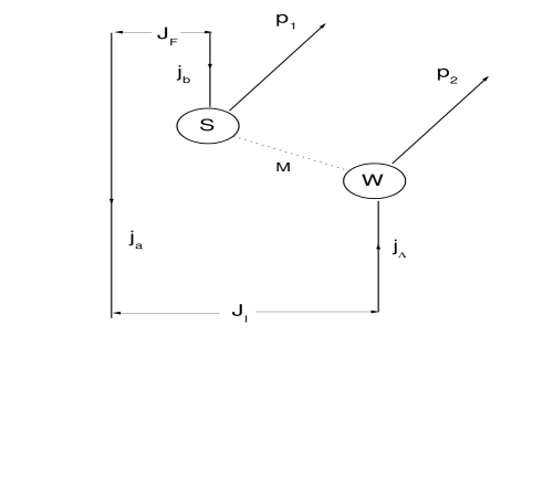
FIG. 1.: Diagramatic representation of the hypernuclear NM weak decay, from the 1p1h state $|j_{\Lambda}j^{-1}_{a};J_{I}\rangle$ to the 2h state $|j_{a}^{-1}j_{b}^{-1}J_{F}\rangle$, while two nucleons with momenta ${\bf p}_{1}$ and ${\bf p}_{2}$ are emitted into the continuum. S and W are the strong and the weak vertices, respectively, and M is a non-strange meson.

The simplest nuclear shell model is the EPHM, in which: the hypernucleus ${}^{A}_{\Lambda}Z$ is described as a $\Lambda$-hyperon in the single particle state $|j_{\Lambda}\rangle$ and a hole state $|{j_{a}}^{-1}\rangle$ relative to the ${}^{A}Z$ core, while the residual ${}^{A-2}Z$ and ${}^{A-2}(Z-1)$ nuclei are represented by the two hole states $|{j_{a}}^{-1}{j_{b}}^{-1}\rangle$ with respect to the same core. As illustrated in Fig. 1 $|J_{I}\rangle\rightarrow|j_{\Lambda}j^{-1}_{a};J_{I}\rangle$, $|J_{F}\rangle\rightarrow|{j_{a}}^{-1}{j_{b}}^{-1};J_{F}\rangle$ and $|J_{C}\rangle\rightarrow|{j_{a}}^{-1}\rangle$. The parentage coefficients in (LABEL:2.17) read

$$\langle J_{C}||a_{j_{b}m_{t_{b}}}^{\dagger}||J_{F}\rangle=(-)^{J_{F}+j_{a}+j_{b}}\sqrt{1+\delta_{ab}}\hat{J}_{F}.$$ (109)

In particular, for ${}^{12}_{\Lambda}C$ the initial state is

$$\left(a_{j_{\Lambda}}^{\dagger}\overline{a}_{j_{a}}\right)_{J_{I}}|0\rangle\equiv|j_{\Lambda}j^{-1}_{a};J_{I}\rangle=|1s_{1/2}\Lambda,1p_{3/2}n^{-1};1\rangle,$$ (110)

and the final states are:

$$\left(\overline{a}_{j_{a}}\overline{a}_{j_{b}}\right)_{J_{F}}|0\rangle\equiv|{j_{a}}^{-1}{j_{b}}^{-1};J_{F}\rangle=\left\{\begin{array}[]{ll}|(1p_{3/2}n^{-1})^{2};0,2\rangle,|1p_{3/2}n^{-1}1s_{1/2}n^{-1};1,2\rangle,\\ \\ |(1p_{3/2}n^{-1}1p_{3/2}p^{-1});0,1,2,3\rangle,|1p_{3/2}n^{-1}1s_{1/2}p^{-1};1,2\rangle,\\ \end{array}\right.$$ (114)

for $\Lambda n\rightarrow nn$ and $\Lambda p\rightarrow np$, respectively. Here $|0\rangle$ is the ${}^{12}C$ particle vacuum. As there is only one hole state for each parity, the parentage coefficients with different $j_{b}=j_{N}$ do not interfere among themselves. After summing up on the final states the integrand (LABEL:2.17) can be cast in the form

$${{\cal I}}_{m_{t_{b}}}(p,P)=\sum_{j_{b}J}F_{m_{t_{b}}J}^{j_{b}}(p_{3/2})\sum_{S\lambda lLT}{{\cal M}}^{2}(pPlL\lambda SJT;{j_{\Lambda}j_{b},m_{t_{b}}}),$$ (115)

where

$$F_{m_{t_{b}}J}^{j_{b}}(j_{a}) = \hat{J}^{2}\hat{j}_{b}^{-2}\sum_{J_{F}=|j_{a}-j_{b}|}^{j_{a}+j_{b}}\left[1+(-)^{J_{F}}\delta_{j_{a}j_{b}}\delta_{m_{t_{b}}m_{t_{a}}}\right]\hat{J}_{F}^{2}\left\{\negthinspace\begin{array}[]{ccc}j_{a}&j_{b}&J_{F}\\ J&J_{I}&j_{\Lambda}\end{array}\right\}^{2}.$$ (118)

are geometrical factors which come from the Pauli principle. Their explicit values for the $1s_{1/2},1p_{3/2},1p_{1/2}$ are listed in Table II.

TABLE II.: Geometrical factors $\hat{j}_{b}^{2}F^{j_{b}}_{m_{t_{b}J}}(j_{a})$

$j_{a}$	$j_{b}$	J	$neutrons$	$protons$
$1p_{3/2}$	$1s_{1/2}$	$0$	$1$	$1$
		$1$	$3$	$3$
$1p_{1/2}$	$1s_{1/2}$	$0$	$1$	$1$
		$1$	$3$	$3$
$1p_{3/2}$	$1p_{3/2}$	$1$	$7$	$6$
		$2$	$5$	$10$
$1p_{1/2}$	$1p_{3/2}$	$1$	$6$	$6$
		$2$	$10$	$10$
$1p_{3/2}$	$1p_{1/2}$	$0$	$1$	$1$
		$1$	$3$	$3$
$1p_{1/2}$	$1p_{1/2}$	$0$	$0$	$1$
		$1$	$2$	$3$

B Beyond Extreme Particle-Hole Model

The EPHM can be straightforwardly improved by going to the quasiparticle representation. In fact, for all even-mass hypernuclei the initial and final states can be expressed as:

$$|J_{I}\rangle = \sum_{j_{\Lambda}j_{a}}C_{j_{\Lambda}j_{a}}\left(a_{j_{\Lambda}}^{\dagger}b^{\dagger}_{j_{a}}\right)_{J_{I}}|BCS\rangle,$$ (119)

$$|J_{F}^{\alpha}\rangle = \sum_{j_{a}j_{b}}C_{j_{a}j_{b}J_{F}}^{\alpha}\left(b_{j_{a}}^{\dagger}b^{\dagger}_{j_{b}}\right)_{J_{F}}|BCS\rangle,$$ (120)

where $b_{j}^{\dagger}=u_{j}a_{j}^{\dagger}-v_{j}a_{\overline{j}}$ is the quasiparticle creation operator [48], $|BCS\rangle$ is the BCS vacuum, $j_{a}$ is always a neutron state, while $j_{b}$ can be both a neutron and a proton orbital. Note that because of the lack of hyperon-hole states, the backward going RPA contributions do not appear and one has to work within the QTDA. From (LABEL:2.13) we get

$${{\cal I}}_{m_{t_{b}}}(p,P)=\sum_{lL\lambda SJJ_{F}^{\alpha}T}\hat{J}^{2}\hat{J}_{F}^{2}$$ (121)

$$\times \left|\sum_{j_{\Lambda}j_{a}j_{b}}(-)^{j_{a}+j_{b}}\sqrt{1+\delta_{ab}}C^{\alpha}_{j_{a}j_{b}J_{F}}C_{j_{a}j_{\Lambda}}v_{j_{b}}{{\cal M}}(pPlL\lambda SJT;j_{\Lambda}j_{b},m_{t_{b}})\left\{\negthinspace\begin{array}[]{ccc}j_{a}&J_{I}&j_{\Lambda}\\ J&j_{b}&J_{F}\end{array}\right\}\right|^{2}.$$ (124)

The residual interaction in the final nuclei redistributes the transition rates among the states with the same spin and parity. But, as the NM decay is an inclusive process, i.e., the partial transition rates are summed up coherently over all final states, such a rearrangement plays only a very minor role on the total rates. (The same happens, for instance, in the neutrino-nucleus reactions and in the $\mu$ meson capture [51].) Therefore, it is justifiable to approximate the final wave functions by their unperturbed forms, i.e., $|J_{F}^{\alpha}\rangle\equiv\left(b_{j_{a}}^{\dagger}b^{\dagger}_{j_{b}}\right)_{J_{F}}|BCS\rangle$ and $C^{\alpha}_{j_{a}j_{b}J_{F}}\equiv\delta_{\alpha,{j_{a}j_{b}}}$. If, in addition, one assumes that the hyperon is always in the lowest $1s_{1/2}$ state the last equation takes the form of (115), i.e.,

$${{\cal I}}_{m_{t_{b}}}(p,P)=\sum_{j_{a}j_{b}J}F_{m_{t_{b}}J}^{j_{b}}(j_{a})C^{2}_{j_{a}j_{\Lambda}}v^{2}_{j_{b}}\sum_{S\lambda lLT}{{\cal M}}^{2}(pPlL\lambda SJT;{j_{\Lambda}j_{b},m_{t_{b}}}),$$ (126)

Only the orbitals $1s_{1/2}$, $1p_{3/2}$ and $1p_{1/2}$ will be used. In this case, as seen from Table II, $F_{pJ}^{j_{b}}(p_{1/2})=F_{pJ}^{j_{b}}(p_{3/2})$, which implies that in the case of protons the summation on $j_{a}$ can be performed analytically. Thus, as $\sum_{j_{a}}C^{2}_{j_{a}j_{\Lambda}}=1$, one finds out that $\Gamma_{p}$ does not depend at all on the initial wave function. From the same table one also finds out that $F_{nJ}^{j_{b}}(j_{a})=F_{pJ}^{j_{b}}(j_{a})$, except when $j_{b}=j_{a}$. So, one can expect as well only a weak dependence of $\Gamma_{n}$ on $|J_{I}\rangle$. This fact is verified numerically later on.

In summary, we end up with a very simple result for the transition rates:

$$\Gamma_{m_{t_{b}}} = \sum_{j_{b}J}v^{2}_{j_{b}}F_{m_{t_{b}}J}^{j_{b}}(j_{a}){{\cal R}}_{m_{t_{b}}J}^{j_{b}},$$ (127)

where

$${{\cal R}}_{m_{t_{b}}J}^{j_{b}}=\frac{16M_{N}^{3}}{\pi}\int_{0}^{\Delta_{j_{b}}}d{\epsilon}\sqrt{{\epsilon}(\Delta_{j_{b}}-{\epsilon})}\sum_{SlL\lambda T}{{\cal M}}^{2}(pPlL\lambda SJT;{j_{\Lambda}j_{b},m_{t_{b}}}).$$ (128)

Clearly, the EPHM is contained in (127) with the occupation numbers $v_{j_{b}}$ equal to one for the occupied states and to zero for the empty states.

C Multipole Expansion

The EPHM is particularly suitable for performing the multipole expansion of the integrands ${{\cal I}}_{m_{t_{b}}}$. Thus we carry out both the Racah algebra in (22) and the summations indicated in (115), keeping in mind that the allowed quantum numbers $\{{\sf lL}\}$ are: $\{00\}$ for the $s_{1/2}$ state, and $\{01\}$ and $\{10\}$ for the $p_{3/2}$ state. To simplify the results we take advantage of the relations

$$(P0|10) = \left(\frac{\pi}{2}\right)^{1/4}b^{3/2}e^{-(Pb)^{2}/4},$$ (129)

$$(P1|11) = \frac{1}{\sqrt{3}}\left(\frac{\pi}{2}\right)^{1/4}b^{5/2}Pe^{-(Pb)^{2}/4},$$ (130)

for the radial integrals $(PL|{\sf{NL}})$ defined in (195), and introduce the ratio

$$R=\frac{(bP)^{2}}{3}\equiv\left[\frac{(P1|11)}{(P0|10)}\right]^{2},$$ (131)

which allows us to work only with the ${\sf L}=0$ overlap $(P0|10)$. Thus, from now on the label ${\sf L}$ will be disregarded, and to identify the $s_{1/2}$ and $p_{3/2}$ pieces of the ${\sf l}=0$ strength we will use the ratio $R$, which appears only in the last term of (115). The results of the multipole expansion for both PC and PV potentials are displayed below.

1 Parity conserving contributions

The matrix elements of the PC operators $f_{M}(r)$, $f^{S}_{M}(r)(\mbox{\boldmath$\sigma$}_{\Lambda}\cdot\mbox{\boldmath$\sigma$}_{N})$, and $f^{T}_{M}(r)S_{\Lambda N}(\hat{r})$, given by (LABEL:A1), can be expressed by means of the radial matrix elements (195) and (196), or more precisely through the moments

$${\sf C}_{M}^{{\sf l}}(p,P) = {{\cal B}}^{\prime}_{M}(p{\sf l}|f_{M}|1{\sf l})(P0|10),$$ (132)

$${\sf S}_{M}^{{\sf l}}(p,P) = {{\cal B}}_{M}{(p{\sf l}|f^{S}_{M}|1{\sf l})}(P0|10)\times\left\{\begin{array}[]{rcc}1&\mbox{for}&\pi,\eta,K\\ 2&\mbox{for}&\rho,\omega,K^{*}\end{array}\right.,$$ (135)

$${\sf T}_{M}^{l{\sf l}}(p,P) = {{\cal B}}_{M}{(pl|f^{T}_{M}|1{\sf l})}(P0|10)\times\left\{\begin{array}[]{rcc}1&\mbox{for}&\pi,\eta,K\\ -1&\mbox{for}&\rho,\omega,K^{*}\end{array}\right..$$ (138)

Introducing the notation:

$$\begin{array}[]{ccc}\underline{\tau=0}&&\underline{\tau=1}\\ {\sf C}_{0}={\sf C}_{\omega}+{\sf C}_{K_{0}}&;&{\sf C}_{1}={\sf C}_{\rho}+{\sf C}_{K^{*}_{1}},\\ {\sf S}_{0}={\sf S}_{\eta}+{\sf S}_{\omega}+{\sf S}_{K_{0}}+{\sf S}_{K^{*}_{0}}&;&{\sf S}_{1}={\sf S}_{\pi}+{\sf S}_{\rho}+{\sf S}_{K_{1}}+{\sf S}_{K^{*}_{1}},\\ {\sf T}_{0}={\sf T}_{\eta}+{\sf T}_{\omega}+{\sf T}_{K_{0}}+{\sf T}_{K^{*}_{0}}&;&{\sf T}_{1}={\sf T}_{\pi}+{\sf T}_{\rho}+{\sf T}_{K_{1}}+{\sf T}_{K^{*}_{1}},\\ \end{array}$$ (143)

for the isoscalar ($\tau=0$) and the isovector ($\tau=1$) matrix elements, one gets:

$${\cal I}_{p} = 2\left(1+R\right)\left[3\left({\sf S}^{0}_{0}\right)^{2}+9\left({\sf S}^{0}_{1}\right)^{2}+\left({\sf C}^{0}_{0}\right)^{2}+7\left({\sf C}^{0}_{1}\right)^{2}+6\left(3{\sf T}^{20}_{1}-{\sf T}^{20}_{0}\right)^{2}\right.$$ (144)

$$- \left.4{\sf C}^{0}_{0}{\sf C}^{0}_{1}+12{\sf C}^{0}_{1}{\sf S}^{0}_{1}-6{\sf C}^{0}_{0}{\sf S}^{0}_{1}-6{\sf C}^{0}_{1}{\sf S}^{0}_{0}\right]$$ (145)

$$+ 6\left({\sf S}^{1}_{0}\right)^{2}+42\left({\sf S}^{1}_{1}\right)^{2}-24{\sf S}^{1}_{0}{\sf S}^{1}_{1}+2\left({\sf C}^{1}_{0}\right)^{2}+6\left({\sf C}^{1}_{1}\right)^{2}-24{\sf C}^{1}_{1}{\sf S}^{1}_{1}$$ (146)

$$+ 12{\sf C}^{1}_{1}{\sf S}^{1}_{0}+12{\sf C}^{1}_{0}{\sf S}^{1}_{1}+\frac{6}{5}\left({\sf T}^{11}_{0}+{\sf T}^{11}_{1}\right)^{2}+\frac{54}{5}\left({\sf T}^{31}_{0}+{\sf T}^{31}_{1}\right)^{2},$$ (147)

for the decay $\Lambda p\rightarrow np$, and

$${\cal I}_{n} = \left(1+\frac{7R}{3}\right)\left(3{\sf S}^{0}_{0}+3{\sf S}^{0}_{1}-{\sf C}^{0}_{0}-{\sf C}^{0}_{1}\right)^{2}+\frac{11}{6}\left({\sf S}^{1}_{0}+{\sf C}^{1}_{0}+{\sf S}^{1}_{1}+{\sf C}^{1}_{1}\right)^{2}$$ (148)

$$+ \frac{38}{15}\left({\sf T}^{11}_{0}+{\sf T}^{11}_{1}\right)^{2}+\frac{54}{5}\left({\sf T}^{31}_{0}+{\sf T}^{31}_{1}\right)^{2},$$ (149)

for the decay $\Lambda n\rightarrow nn$.

2 Parity violating contributions

The PV matrix elements (207) are reduced to the nuclear moments

$${\sf P}_{M}^{l{\sf l}}(p,P) = {{\cal A}}_{M}{(pl|f^{(-)}_{M}|1{\sf l})}(P0|10),$$ (150)

$${\sf Q}_{M}^{l{\sf l}}(p,P) = {{\cal A}}^{\prime}_{M}{(pl|f^{(+)}_{M}|1{\sf l})}(P0|10),$$ (151)

where the radial integrals $(pl|f^{(\pm)}_{M}|1{\sf l})$ are defined in (212). Using the notation,

$$\widetilde{{\sf P}}_{\eta} = {\sf P}_{\eta}-{\sf Q}_{K_{0}^{*}},~{}~{}\widetilde{{\sf P}}_{K_{0}}={\sf P}_{K_{0}}-{\sf Q}_{\omega},~{}~{}\widetilde{{\sf P}}_{K_{0}^{*}}={\sf P}_{K_{0}^{*}}+{\sf P}_{\omega},$$ (152)

$$\widetilde{{\sf P}}_{\pi} = {\sf P}_{\pi}-{\sf Q}_{K_{1}^{*}},~{}~{}\widetilde{{\sf P}}_{K_{1}}={\sf P}_{K_{1}}-{\sf Q}_{\rho},~{}~{}\widetilde{{\sf P}}_{K_{1}^{*}}={\sf P}_{K_{1}^{*}}+{\sf P}_{\rho},$$ (153)

we obtain:

$${\cal I}_{p} = 2\left(1+R\right)\left[3\left(\widetilde{{\sf P}}^{10}_{\pi}\right)^{2}+\left(\widetilde{{\sf P}}^{10}_{\eta}\right)^{2}+3\left(\widetilde{{\sf P}}^{10}_{K_{1}}\right)^{2}+\left(\widetilde{{\sf P}}^{10}_{K_{0}}\right)^{2}+10\left(\widetilde{{\sf P}}^{10}_{K_{1}^{*}}\right)^{2}+2\left(\widetilde{{\sf P}}^{10}_{K_{0}^{*}}\right)^{2}\right.$$ (154)

$$- \left.2\widetilde{{\sf P}}^{10}_{\eta}\widetilde{{\sf P}}^{10}_{K_{1}}+2\widetilde{{\sf P}}^{10}_{\pi}\left(2\widetilde{{\sf P}}^{10}_{K_{1}}-\widetilde{{\sf P}}^{10}_{K_{0}}+4\widetilde{{\sf P}}^{10}_{K_{1}^{*}}-2\widetilde{{\sf P}}^{10}_{K_{0}^{*}}\right)+4\widetilde{{\sf P}}^{10}_{K_{1}}(2\widetilde{{\sf P}}^{10}_{K_{1}^{*}}-\widetilde{{\sf P}}^{10}_{K_{0}^{*}})-4\widetilde{{\sf P}}^{10}_{K_{1}^{*}}\widetilde{{\sf P}}^{10}_{K_{0}^{*}}\right]$$ (155)

$$+ 14\left(\widetilde{{\sf P}}^{21}_{\pi}\right)^{2}+2\left(\widetilde{{\sf P}}^{21}_{\eta}\right)^{2}+8\left(\widetilde{{\sf P}}^{21}_{K_{1}}\right)^{2}+\frac{4}{3}\left(\widetilde{{\sf P}}^{21}_{K_{0}}\right)^{2}+14\left(\widetilde{{\sf P}}^{21}_{K_{1}^{*}}\right)^{2}+\frac{10}{3}\left(\widetilde{{\sf P}}^{21}_{K_{0}^{*}}\right)^{2}$$ (156)

$$+ 4\widetilde{{\sf P}}^{21}_{\eta}\widetilde{{\sf P}}^{21}_{K_{1}}-4\widetilde{{\sf P}}^{21}_{\pi}\left(2\widetilde{{\sf P}}^{21}_{K_{0}^{*}}+2\widetilde{{\sf P}}^{21}_{K_{1}}-\widetilde{{\sf P}}^{21}_{K_{0}}+4\widetilde{{\sf P}}^{21}_{K_{1}^{*}}-2\widetilde{{\sf P}}^{21}_{K_{0}^{*}}\right)+4\widetilde{{\sf P}}^{21}_{K_{1}}\left(\widetilde{{\sf P}}^{21}_{\eta}-\widetilde{{\sf P}}^{21}_{K_{1}^{*}}+\widetilde{{\sf P}}^{21}_{K_{0}^{*}}\right)$$ (157)

$$+ 4\widetilde{{\sf P}}^{21}_{K_{1}^{*}}\left(2\widetilde{{\sf P}}^{21}_{\eta}-\widetilde{{\sf P}}^{21}_{K_{0}^{*}}\right)+\frac{4}{3}\widetilde{{\sf P}}^{21}_{K_{0}^{*}}\widetilde{{\sf P}}^{21}_{K_{0}}$$ (158)

$$+ \frac{2}{3}\left(\widetilde{{\sf P}}^{01}_{K_{0}}\right)^{2}+6\left(\widetilde{{\sf P}}^{01}_{K_{1}}\right)^{2}+\frac{2}{3}\left(\widetilde{{\sf P}}^{01}_{K_{0}^{*}}\right)^{2}+6\left(\widetilde{{\sf P}}^{01}_{K_{1}^{*}}\right)^{2}-4\widetilde{{\sf P}}^{01}_{K_{0}}\widetilde{{\sf P}}^{01}_{K_{1}}$$ (159)

$$- \frac{4}{3}\widetilde{{\sf P}}^{01}_{K_{0}^{*}}\left(\widetilde{{\sf P}}^{01}_{K_{0}}-3\widetilde{{\sf P}}^{01}_{K_{1}}+3\widetilde{{\sf P}}^{01}_{K_{1}^{*}}\right)+4\widetilde{{\sf P}}^{01}_{K_{1}^{*}}\left(\widetilde{{\sf P}}^{01}_{K_{0}}-3\widetilde{{\sf P}}^{01}_{K_{1}}\right),$$ (160)

for the $\Lambda p\rightarrow np$ decay, and

$${\cal I}_{n} = \left(3+\frac{43R}{18}\right)\left[\left(\widetilde{{\sf P}}_{\pi}^{10}+\widetilde{{\sf P}}_{\eta}^{10}\right)^{2}+\left(\widetilde{{\sf P}}_{K_{0}}^{10}+\widetilde{{\sf P}}_{K_{1}}^{10}\right)^{2}\right]+\left(4+\frac{14R}{3}\right)\left(\widetilde{{\sf P}}_{K_{0}^{*}}^{10}+\widetilde{{\sf P}}_{K_{1}^{*}}^{10}\right)^{2}$$ (162)

$$- \left(2+\frac{R}{9}\right)\left(\widetilde{{\sf P}}_{\pi}^{10}+\widetilde{{\sf P}}_{\eta}^{10}\right)\left(\widetilde{{\sf P}}_{K_{0}}^{10}+\widetilde{{\sf P}}_{K_{1}}^{10}\right)$$ (163)

$$- \left(4+\frac{14R}{3}\right)\left(\widetilde{{\sf P}}_{K_{0}^{*}}^{10}+\widetilde{{\sf P}}_{K_{1}^{*}}^{10}\right)\left(\widetilde{{\sf P}}_{\pi}^{10}+\widetilde{{\sf P}}_{\eta}^{10}+\widetilde{{\sf P}}_{K_{0}}^{10}+\widetilde{{\sf P}}_{K_{1}}^{10}\right)$$ (164)

$$+ \frac{1}{2}\left(\widetilde{{\sf P}}_{\pi}^{21}+\widetilde{{\sf P}}_{\eta}^{21}+\widetilde{{\sf P}}_{K_{0}}^{21}+\widetilde{{\sf P}}_{K_{1}}^{21}\right)^{2}$$ (165)

$$+ 2\left(\widetilde{{\sf P}}_{K_{0}^{*}}^{21}+\widetilde{{\sf P}}_{K_{1}^{*}}^{21}\right)\left(\widetilde{{\sf P}}_{K_{0}^{*}}^{21}+\widetilde{{\sf P}}_{K_{1}^{*}}^{21}+\widetilde{{\sf P}}_{\pi}^{21}+\widetilde{{\sf P}}_{\eta}^{21}+\widetilde{{\sf P}}_{K_{0}}^{21}+\widetilde{{\sf P}}_{K_{1}}^{21}\right),$$ (166)

for the $\Lambda n\rightarrow nn$ decay.

V Numerical Results and Discussion

The numerical values of the parameters, defined in Table I and necessary to specify the transition potential, are summarized in Table III. For the sake of comparison all cutoffs appearing in (170), as well as all coupling constants, were taken from Ref. [13], where, in turn, the strong couplings have been taken from Refs. [28, 29] and the weak ones from Ref. [12]. The energy difference $\Delta_{j_{N}m_{t_{N}}}$ in (37) is evaluated from the experimental single nucleon and hyperon energies, quoted in Ref. [8].

TABLE III.: Parameters used in the calculations: masses (in MeV), cut-offs (in GeV) and the isoscalar ($\tau=0$) and isovector ($\tau=1$) coupling constants (in units of $10^{-11}$ MeV^-2).

M	$m_{M}$	$\Lambda$	${{\cal A}}_{M}/m_{M}$	${{\cal A}}^{\prime}_{M}/m_{M}$	${{\cal B}}_{M}$	${{\cal B}}^{\prime}_{M}/m_{M}^{2}$
			$\tau=0$
$\eta$	$548.6$	$1.3$	$0.247$		$-0.525$
$K$	$495.8$	$1.2$	$-0.828$		$0.228$
$\omega$	$783.4$	$1.5$	$-0.274$	$-0.420$	$-0.923$	$-1.395$
$K^{*}$	$892.4$	$2.2$	$0.376$	$0.237$	$0.632$	$1.016$
			$\tau=1$
$\pi$	$140.0$	$1.3$	$1.175$		$-0.546$
$K$	$495.8$	$1.2$	$-0.127$		$0.764$
$\rho$	$775.0$	$1.4$	$0.273$	$0.105$	$-0.907$	$-0.407$
$K^{*}$	$892.4$	$2.2$	$0.514$	$0.324$	$1.072$	$0.274$

The finite nucleon size (FNS) effects at the interaction vertices are gauged by the monopole form factor $F_{M}^{\rm(FNS)}({\bf q}^{2})=\displaystyle\frac{\Lambda_{M}^{2}-m_{M}^{2}}{\Lambda_{M}^{2}+{\bf q}^{2}}$, which implies that the propagators in (73) and (76) must be replaced by

$$f_{M}(r)\rightarrow\overline{f}_{M}(r) = f_{M}(r)-f_{\Lambda_{M}}(r)-\frac{r(\Lambda_{M}^{2}-m_{M}^{2})}{2\Lambda_{M}}f_{\Lambda_{M}}(r),$$ (167)

$$f^{S}_{M}(r)\rightarrow\overline{f}^{S}_{M}(r) = f^{S}_{M}(r)-f^{S}_{\Lambda_{M}}(r)-\frac{1}{6}(\Lambda_{M}^{2}-m_{M}^{2})(\Lambda_{M}r-2)f_{\Lambda_{M}}(r),$$ (168)

$$f^{T}_{M}(r)\rightarrow\overline{f}^{T}_{M}(r) = f^{T}_{M}(r)-f^{T}_{\Lambda_{M}}(r)-\frac{1}{6}(\Lambda_{M}^{2}-m_{M}^{2})(\Lambda_{M}r+1)f_{\Lambda_{M}}(r),$$ (169)

$$f^{\prime}_{M}(r)\rightarrow\overline{f}^{\prime}_{M}(r) = f^{\prime}_{M}(r)-f^{\prime}_{\Lambda_{M}}(r)+\frac{r(\Lambda_{M}^{2}-m_{M}^{2})}{2}f_{\Lambda_{M}}(r),$$ (170)

where $f_{\Lambda_{M}}(r)$ has the same structure as ${f}_{M}(r)$ but with $m_{M}\rightarrow\Lambda_{M}$.

The initial and final short range correlations (SRC) are taken into account, respectively, via the correlation functions [13],

$$g_{i}(r) = \left(1-e^{-r^{2}/\alpha^{2}}\right)^{2}+\beta r^{2}e^{-r^{2}/\gamma^{2}},$$ (171)

$$g_{f}(r) = 1-j_{0}(q_{c}r),$$ (172)

with $\alpha=0.5$ fm, $\beta=0.25$ fm^-2, and $\gamma=1.28$ fm, and $q_{c}=3.93$ fm^-1.

It is a general belief nowadays that, in any realistic evaluation of the hypernuclear NM decay, the FNS and SRC have to be included simultaneously. Therefore, in the present paper we will discuss only the numerical results, in which both of these renormalization effects are considered. Under these circumstances, and because of the relative smallness of pion mass, the transition is dominated by the OPE [13].

TABLE IV.: Parity conserving (PC) and parity violating (PV) nonmesonic decay rates for ${}^{12}_{\Lambda}C$, in units of $\Gamma^{0}=2.50\cdot 10^{-6}$ eV. All coupling constants and the cutoff parameters are from Table III and $b=1.51$ fm. All calculations were done within the EPHM, except for a few results which were evaluated in the QTDA and are shown parenthetically.

Mesons	$\Gamma_{n}^{\scriptstyle\rm PC}$	$\Gamma_{n}^{\scriptstyle\rm PV}$	$\Gamma_{p}^{\scriptstyle\rm PC}$	$\Gamma_{p}^{\scriptstyle\rm PV}$
$\pi$	$0.009$	$0.151$	$0.734$	$0.383$
	($0.016$)	($0.153$)	($0.732$)	($0.373$)
$\eta$	$0.003$	$0.004$	$0.006$	$0.003$
$K$	$0.008$	$0.069$	$0.097$	$0.043$
$\rho$	$0.005$	$0.003$	$0.109$	$0.008$
$\omega$	$0.004$	$0.007$	$0.066$	$0.004$
$K^{*}$	$0.025$	$0.034$	$0.056$	$0.028$
$\pi+\eta$	$0.013$	$0.204$	$0.630$	$0.383$
$\pi+K$	$0.013$	$0.258$	$0.325$	$0.512$
$\pi+\rho$	$0.009$	$0.133$	$0.583$	$0.461$
$\pi+\omega$	$0.015$	$0.176$	$0.902$	$0.406$
$\pi+K^{*}$	$0.044$	$0.075$	$1.020$	$0.455$
$\pi+\eta+K$	$0.008$	$0.318$	$0.259$	$0.505$
	($0.011$)	($0.330$)	($0.258$)	($0.516$)
$\pi+\eta+K+K^{*}$	$0.052$	$0.268$	$0.486$	$0.602$
all mesons	$0.037$	$0.240$	$0.347$	$0.714$
	($0.039$)	($0.250$)	($0.346$)	($0.702$)

The major part of the numerical calculations were done in the EPHM where the only free parameter is the harmonic oscillator length $b$. The most commonly used estimate is $b=A^{1/6}$ fm [49, 48], which corresponds to the oscillator energy $\hbar\omega=41A^{-1/3}$ MeV, and gives $b=1.51$ fm. For light nuclei it is sometimes preferred to employ $\hbar\omega=45A^{-1/3}-25A^{-2/3}$ MeV, which yields $b=1.70$ fm. Moreover, a $\Lambda$ particle in a hypernucleus is typically less bound than the corresponding nucleon and hence $b_{\Lambda}$ could be larger than $b_{N}$. For instance, in Ref. [13] was used $b=(b_{\Lambda}+b_{N})/2=1.75$ fm, which comes from $b_{N}=1.64$ fm and $b_{\Lambda}=1.87$ fm. As there is no deep motivation for preferring one particular value of $b$, the numerical results will be exhibited for both $b=1.51$ fm and $b=1.75$ fm.

First, a few illustrative results, obtained in the EPHM (Eq. (115)) and the simplified version of the QTDA (Eq. (126)), are displayed in the Table IV. The hyperon-nucleon interaction in the later approach was taken to be a simple $\delta$ force, which has been recently used with success as the nucleon-nucleon interaction to explain the weak decay processes in ${}^{12}C$ [51]. The resulting pairing BCS factors were: $v_{s_{1/2}}=0.9868$, $v_{p_{3/2}}=0.8978$ and $v_{p_{1/2}}=0.6439$. Although we have expected to obtain small differences between the EPHM and the QTDA, it came as a surprise that they turned out to be so tiny. Thus, henceforth only the first one will be used.

Next, we combine results from Table IV with the multipole expansion done in the previous section to find out the roles played by different mesons. Note that the formulas (LABEL:N.14) and (166) depend on the ratio (131), and it was found numerically that the approximation

$$R=1,$$ (173)

reproduces fairly well the exact calculations. This estimate helped us to formulate the following comments:

PC potential; The dominant contributions to $\Gamma_{p}$ and $\Gamma_{n}$ come from the ${\sf l}=0$ matrix elements, while the ${\sf l}=1$ wave contributes relatively little: $\cong 2\%$ to $\Gamma_{p}$ and $\cong 10\%$ to $\Gamma_{n}$. On the other hand, for the parametrization displayed in Table III, one finds that: (1) the $\omega$ and $K^{*}$ mesons mainly cancel out in ${\sf C}^{0}_{0}$, as the $\rho$ and $K^{*}$ mesons do in ${\sf C}^{0}_{1}$, and (2) the matrix elements ${\sf S}^{0}_{0}$ and ${\sf S}^{0}_{1}$ are small in comparison with $(3{\sf T}^{20}_{1}-{\sf T}^{20}_{0})$, which makes $\Gamma_{p}$ to be large vis-$\grave{a}$-vis $\Gamma_{n}$. Thus, using the estimate (173), one ends up with the following approximate result for the PC contributions:

$${\cal I}_{p}+{\cal I}_{n} \cong {\cal I}_{p}\cong 2{{\cal I}}_{p}^{s_{1/2}}\cong\ 24\left(3{\sf T}^{20}_{1}-{\sf T}^{20}_{0}\right)^{2}.$$ (174)

From Table III and (143) one can also see that: (i) the $\omega$ and $K^{*}$ mesons contribute coherently with the pion, while the remaining three mesons contribute out of phase, and (ii) the different vector meson contributions have the tendency to cancel among themselves. As is shown in Table IV, the overall effect is a reduction of the pion transition rate by approximately a factor of two.

PV potential; As in the PC case, the dominant PV transition strengths come from the ${\sf l}=0$ wave, through the $\widetilde{{\sf P}}^{10}_{M}$ moments. The ${\sf l}=1$ wave from the $p_{3/2}$ state gives rise to $l=0$ and $l=2$ outgoing channels. The first one can always be neglected, while the second one contributes with $15\%$ to $\Gamma_{p}$ and with $2\%$ to $\Gamma_{n}$, when only the $\pi$ meson is considered. After including all mesons these percentages drop to $6\%$ and $1\%$, respectively. Also here the partial $s_{1/2}$ and $p_{3/2}$ contributions are approximately equal for all mesons in the proton induced channel and notably different in the neutron induced channel.

From Table IV it is easily found that the most important PV contributions arise from the ${\sf P}^{10}_{\pi}$ moment, and from its interference with the ${\sf P}^{10}_{\eta}$, ${\sf P}^{10}_{K}$ and ${\sf P}^{10}_{K^{*}}$ moments. Thus, retaining only the most relevant terms in (LABEL:N.14) and (166), the following rough estimates are obtained:

$${\cal I}_{p}\cong 2{{\cal I}}_{p}^{s_{1/2}} \cong 4\left[3\left({\sf P}^{10}_{\pi}\right)^{2}+3\left({\sf P}^{10}_{K_{1}}\right)^{2}+\left({\sf P}^{10}_{K_{0}}\right)^{2}\right]$$ (176)

$$+8{\sf P}^{10}_{\pi}\left(2{\sf P}^{10}_{K_{1}}-{\sf P}^{10}_{K_{0}}+4{\sf P}^{10}_{K_{1}^{*}}-2{\sf P}^{10}_{K_{0}^{*}}-3{\sf Q}^{10}_{K_{1}^{*}}\right),$$

and

$${\cal I}_{n} \cong \frac{97}{18}\left[\left({\sf P}^{10}_{\pi}\right)^{2}+\left({\sf P}_{K_{1}}^{10}+{\sf P}_{K_{0}}^{10}\right)^{2}\right]-\frac{19}{9}{\sf P}^{10}_{\pi}\left({\sf P}_{K_{1}}^{10}+{\sf P}_{K_{0}}^{10}\right)$$ (178)

$$+\frac{97}{9}{\sf P}^{10}_{\pi}\left({\sf P}_{\eta}^{10}-{\sf Q}_{K^{*}_{1}}^{10}-{\sf Q}_{K^{*}_{0}}^{10}\right)-\frac{78}{9}{\sf P}^{10}_{\pi}\left({\sf P}_{K^{*}_{1}}^{10}+{\sf P}_{K^{*}_{0}}^{10}\right).$$

These relations are notably more complicated than (174). Nevertheless, it can be concluded that: (1) the $\eta$ meson is only significant for $\Gamma_{n}$, and (2) the $K$ and $K^{*}$ mesons increase both transition rates, but in a different way.

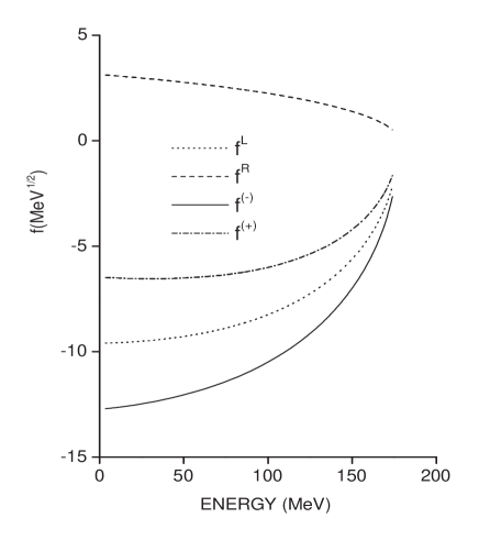
FIG. 2.: Matrix elements of the radial operators $f^{L}_{K^{*}}$, $f^{R}_{K^{*}}$, $f^{(+)}_{K^{*}}$, and $f^{(-)}_{K^{*}}$, as a function of the energy.

Before proceeding it is worth to say a few words on the ”new” nuclear moments ${\sf Q}_{M}^{10}$ and compare them with the well known moments ${\sf P}_{M}^{10}$. As seen from (151) and (212)-(214) they basically differ in the radial dependence. Specifically, we discuss the radial matrix element

$$\overline{(p,1|f^{(+)}_{K^{*}}|10)}=\overline{(p,1|f^{L}_{K^{*}}|10)}+\overline{(p,1|f^{R}_{K^{*}}|10)},$$ (179)

which appears in ${\sf Q}_{K^{*}}^{10}$, together with the usual matrix element

$$\overline{(p,1|f^{(-)}_{K^{*}}|10)}=\overline{(p,1|f^{L}_{K^{*}}|10)}-\overline{(p,1|f^{R}_{K^{*}}|10)},$$ (180)

which is contained in ${\sf P}_{K^{*}}^{10}$. The overline indicates that both the FNS and SRC are included, as explained in the Appendix.

As can be seen from Fig. 2, the matrix elements of $f^{L}_{K^{*}}$ and $f^{R}_{K^{*}}$ have opposite signs, and as a consequence the matrix element of $f^{(-)}_{K^{*}}$ is larger in magnitude than that of $f^{(+)}_{K^{*}}$. A rough approximation for the mean values is:

$$\left|\left<\overline{(p1|f^{(+)}_{K^{*}}|10)}\right>\right|\cong\frac{1}{2}\left|\left<\overline{(p1|f^{(-)}_{K^{*}}|10)}\right>\right|.$$ (181)

As ${{\cal A}}_{K^{*}}\>\raisebox{-2.15277pt}{$\stackrel{{\scriptstyle\textstyle>}}{{\sim}}$}\>{{\cal A}}^{\prime}_{K^{*}}$ (see Table III) we end up with the estimate:

$$\left|\left<{\sf Q}^{10}_{K^{*}}\right>\right|\cong 0.3\left|\left<{\sf P}^{10}_{K^{*}}\right>\right|.$$ (182)

Thus, equations (176) and (178) show that the $K^{*}$ meson mainly contributes through the moments ${\sf P}^{10}_{K^{*}}$, augmenting the magnitude of $\Gamma_{p}^{\scriptstyle\rm PV}$ and diminishing that of $\Gamma_{n}^{\scriptstyle\rm PV}$. The matrix elements ${\sf Q}^{10}_{K^{*}}$, in contrast, reduce both transition rates.

Furthermore, the equation (153) indicates that each vector moment ${\sf Q}^{10}_{\rho,\omega,K^{*}}$ is accompanied by a pseudo-scalar moment ${\sf P}^{10}_{\pi,\eta,K}$. Both integrals $(p1|f_{M}^{(\pm)}|10)$ are negative for all mesons. Then, using the values of the coupling constants ${{\cal A}}_{\pi,\eta,K}$ and ${{\cal A}}^{\prime}_{\rho,\omega,K^{*}}$ listed in Table III, it can be inferred that ${\sf Q}^{10}_{\rho,\omega,K^{*}}$ and ${\sf P}^{10}_{\pi,\eta,K}$ moments mostly add incoherently.

TABLE V.: Parity conserving (PC) and parity violating (PV) nonmesonic decay rates for ${}^{12}_{\Lambda}C$, in units of $\Gamma^{0}=2.50\cdot 10^{-6}$ eV. The data are taken from Refs. [39, 40, 41, 42, 43], and large experimental errors are due to the low efficiencies and large backgrounds in neutron detection. The calculations were performed for both $b=1.51$ fm and $b=1.75$ fm, being the later given parenthetically. In Calculation A all parameters are from Table III, and PS and V stand, respectively, for the pseudo-scalar ($\pi+\eta+K$) and the vector ($\rho+\omega+K^{*}$) mesons, while the label $({\sf P})$ indicates that only the moments ${\sf P}_{M}$ are considered (see (151)). In Calculation B the coupling constants listed in Table III are modified as: ${{\cal A}}_{\eta}\rightarrow 3{{\cal A}}_{\eta}$, ${{\cal A}}_{K_{1}}\rightarrow 5{{\cal A}}_{K_{1}}$, ${{\cal B}}_{\eta}\rightarrow 3{{\cal B}}_{\eta}$ and ${{\cal B}}_{K}\rightarrow 2{{\cal B}}_{K}$, and the signs of all vector meson potentials are inverted.

	$\Gamma_{NM}=\Gamma_{n}+\Gamma_{p}$	$\Gamma_{p}$	$\Gamma_{n/p}=\Gamma_{n}/\Gamma_{p}$
$Measurements$:
Ref. [39]			$0.70\pm 0.3$
Ref. [39]			$0.52\pm 0.16$
Ref. [40]	$1.14\pm 0.2$		$1.33^{+1.12}_{-0.81}$
Ref.[41]	$0.89\pm 0.15\pm 0.03$	$0.31^{+0.18}_{-0.11}$	$1.87\pm 0.59^{+0.32}_{-1.00}$
Ref. [42]	$1.14\pm 0.08$
Ref. [43]			$1.17^{+0.09+0.22}_{-0.08-0.18}$
$Calculation~{}A$:
$\pi$	$1.277(1.006)$	$1.116(0.885)$	$0.143(0.137)$
$PS$	$1.100(0.851)$	$0.774(0.601)$	$0.420(0.416)$
$PS+K^{*}$	$1.408(1.091)$	$1.088(0.846)$	$0.294(0.290)$
$PS+V$	$1.338(1.038)$	$1.061(0.825)$	$0.261(0.259)$
$PS+V({\sf P})$	$1.539(1.190)$	$1.196(0.927)$	$0.287(0.284)$
$Calculation~{}B$:
$PS^{\prime}$	$1.145(0.874)$	$0.555(0.419)$	$1.064(1.089)$
$PS^{\prime}-K^{*}$	$1.273(0.971)$	$0.540(0.407)$	$1.355(1.384)$
$PS^{\prime}-V$	$1.297(0.989)$	$0.542(0.408)$	$1.394(1.423)$

The experimental results for the total transition rate $\Gamma_{NM}$, the proton partial width $\Gamma_{p}$, and the ratio $\Gamma_{n/p}$ in ${}^{12}_{\Lambda}C$ are displayed in Table V. In the same table the theoretical estimates are also shown, grouped as:

1. Calculation A. All the parametrization is taken from Table III, and the following cases are shown and commented:

   • $(\pi)$: The simple OPE model accounts for $\Gamma_{NM}$, but it badly fails regarding $\Gamma_{p}$ and $\Gamma_{n/p}$.

   • $(PS)$: When $\eta$ and $K$ mesons are included, the total transition rate is only slightly modified, while $\Gamma_{p}$ and $\Gamma_{n/p}$ change significantly, coming somewhat closer to the measured values.

   • $(PS+K^{*})$: The incorporation of the $K^{*}$ meson increases $\Gamma_{NM}$ and $\Gamma_{p}$, decreases $\Gamma_{n/p}$, and in this way worsens the agreement with the data.

   • $(PS+V)$: The results are not drastically modified when all vector mesons are built-in.

   • $(PS+V({\sf P}))$: All 6 mesons are included, but only the PV moments ${\sf P}_{M}$ are considered. The importance of the new moments ${\sf Q}_{M}$ is evident from the comparison with the previous case.

   The main conclusion is that it is not possible to reproduce simultaneously the data for all three observables $\Gamma_{NM}$, $\Gamma_{p}$ and $\Gamma_{n/p}$, when the BBM coupling are constrained by the $SU(3)$ and $SU(6)_{w}$ symmetries.

2. Calculation B. We discuss now what happens when the just mentioned constraints are relaxed, and the FNS and SRC parametrizations, as well as the the pion couplings, are kept unchanging. That is, the transition potential is considered to be given by a series of Yukawa like potentials with different spin and isospin dependence. The simple increase of the $K$ coupling does not solve the problem by itself. For instance, for ${{\cal A}}_{K}\rightarrow 2{{\cal A}}_{K}$ and ${{\cal B}}_{K}\rightarrow 2{{\cal B}}_{K}$, the contribution of all three pseudo-scalar mesons is (when $b=1.51$ fm): $\Gamma_{NM}=1.404~{}\Gamma^{0}$, $\Gamma_{p}=0.815~{}\Gamma^{0}$ and $\Gamma_{n/p}=0.723$, and when the vector mesons are added one gets: $\Gamma_{NM}=1.714~{}\Gamma^{0}$, $\Gamma_{p}=1.130~{}\Gamma^{0}$ and $\Gamma_{n/p}=0.518$. Namely, $\Gamma_{NM}$ turns out to be too large. But from the previous discussion, in relation to equations (174), (176) and (178), we have learned that it could be possible to reproduce at the same time the data for all three observables by: (i) making the total tensor interaction in $\Gamma_{p}^{\scriptstyle\rm PC}$ small, and simultaneously (ii) decreasing $\Gamma_{p}^{\scriptstyle\rm PV}$ and increasing $\Gamma_{n}^{\scriptstyle\rm PV}$, without modifying $\Gamma_{\scriptstyle\rm NM}$ too much. The first goal can be accomplished, for instance, through the modifications: ${{\cal B}}_{\eta}\rightarrow 3{{\cal B}}_{\eta}$ and ${{\cal B}}_{K}\rightarrow 2{{\cal B}}_{K}$, and the second one with ${{\cal A}}_{\eta}\rightarrow 3{{\cal A}}_{\eta}$ and ${{\cal A}}_{K_{1}}\rightarrow 5{{\cal A}}_{K_{1}}$. The following cases are illustrated in Table V:

   • $(PS^{\prime})$: Only the pseudoscalar mesons are included with the above changes in $\eta$ and $K$ meson couplings.

   • $(PS^{\prime}-K^{*})$: The $K^{*}$ meson potential is incorporated but with the inverted sign.

   • $(PS^{\prime}-V)$: All vector meson potentials are included with the inverted signs.

No best fit to data has been attempted. Yet, it is clear that there are many other set of parameters that reproduce reasonable well the data. We wish to stress as well that, when the vector mesons are considered, the correct values of $\Gamma_{n/p}$ are obtained only by overturning the signs of the vector meson potentials.

VI Summary and Conclusions

A novel shell model formalism for the nonmesonic weak decay of the hypernuclei has been developed. It involves a partial wave expansion of the emitted nucleon waves and preserves naturally the antisymmetrization between the escaping particles and the residual core. The general expression (LABEL:2.13) is valid for any nuclear model and it shows that the NM transition rates should depend, in principle, on both: (i) the weak transition potential, through the elementary transition amplitudes ${{\cal M}}(pPlL\lambda SJT;{j_{\Lambda}j_{N},m_{t_{N}}})$, and (ii) the nuclear structure, through the two-particle $N\Lambda$ parentage coefficients $\langle J_{I}||\left(a_{j_{N}m_{t_{N}}}^{\dagger}a_{j_{\Lambda}}^{\dagger}\right)_{J}||J_{F}\rangle$. The explicit evaluation of the matrix elements ${{\cal M}}$ is illustrated as well.

Two nuclear models for even-mass hypernuclei, namely the EPHM and the QTDA, were worked out in detail, and the Eqs. (115) and (LABEL:M.2) were derived. The last one explicitly depends on the initial and final wave functions. But, because of: i) the inclusive nature of the nonmesonic decay, and ii) the peculiar properties of the coefficients $F_{m_{t_{b}}J}^{j_{b}}(j_{a})$ this dependence is totally washed out for all practical purposes. In this way we have arrived at a very simple result for transition rates, given by the Eq. (127), which except for the BCS pairing factors $v^{2}_{j_{b}}$, agrees with the EPHM result. Thus, it can be stated that the two-particle correlations in the initial and final state are only of minor importance if of any. With some additional effort can also be incorporated the higher order nuclear structure effects such as the four quasi-particle excitations, collective vibrations, rotations, etc.. Yet, it is hard to imagine a scenario where the later could be relevant at the same time that the former are not. Therefore, we conclude that the nuclear structure manifests basically through the factor $F_{m_{t_{b}}J}^{j_{b}}(j_{a})$, which is engendered by the Pauli principle; $j_{a}$ stands for the hyperon partner in the initial state, and $j_{b}$ runs over all proton and neutron occupied states in the initial nucleus. It is amazing to notice that the Eq. (127) is valid for any even-mass system, which can be so light as ${{}^{4}_{\Lambda}H}$ and ${{}^{4}_{\Lambda}He}$ are or so heavy as ${{}^{208}_{\Lambda}Pb}$ is. (A quite similar result is also obtained for the odd-mass hypernuclei, and this issue will be discussed elsewhere.) One should also add that the last equation contains the same physics as the Eq. (5) in Ref. [13] or the Eq. (30) in Ref. [27], with the advantage that we do not have to deal with spectroscopic factors. Of course, neither the initial and final wave functions are needed.

Attention has been given to the nonrelativistic approximation, used to derive the weak effective hypernuclear one-meson exchange potentials (88) and (99). Same errors and misprints that appear in the recent papers [13, 19, 24] have been corrected. Additional parity violating vector meson operators $\mbox{\boldmath$\sigma$}_{N}\cdot{\bf f}^{(+)}(r)$ and $\mbox{\boldmath$\sigma$}_{\Lambda}\cdot{\bf f}^{(+)}(r)$, usually neglected, have been considered as well. The matrix elements of these new terms were fully discussed, and it was found that they are quite important quantitatively and therefore should not be omitted.

With the OMEM parametrization from the literature [13], and keeping the treatment of the FSI at the simple Jastrow like level ($g(r)=1-j_{0}(q_{c}r)$), we reproduce satisfactorily the data for the total transition rate ($\Gamma_{NM}^{\rm th}\cong\Gamma^{0}$), but the $n/p$-ratio ($\Gamma_{n/p}^{\rm th}\>\raisebox{-2.15277pt}{$\stackrel{{\scriptstyle\textstyle<}}{{\sim}}$}\>0.42$) and the proton partial width ($\Gamma_{p}^{\rm th}\>\raisebox{-2.15277pt}{$\stackrel{{\scriptstyle\textstyle>}}{{\sim}}$}\>0.60\Gamma^{0}$) are not well accounted for. More elaborate treatments of the FSI increase sensibly the $n/p$-ratio, but they are unable to solve the puzzle [13, 24], especially after the last experimental result for this observable [43]. We have found that the new vector meson operators are not of much helpful in this regard either.

Finally, bearing in mind the phenomenological nature of the OMEM, we have also tried to reproduce all three data simultaneously by varying the coupling strengths in a significant way. As the only guide were used the simple formulas (178), (179) and (180), which come out from the multipole expansion done within the EPHM. Such an attempt was successful, and we get: $0.87\>\raisebox{-2.15277pt}{$\stackrel{{\scriptstyle\textstyle<}}{{\sim}}$}\>\Gamma^{\rm th}_{NM}/\Gamma^{0}\>\raisebox{-2.15277pt}{$\stackrel{{\scriptstyle\textstyle<}}{{\sim}}$}\>1.30$, $1.06\>\raisebox{-2.15277pt}{$\stackrel{{\scriptstyle\textstyle<}}{{\sim}}$}\>\Gamma^{\rm th}_{n/p}\>\raisebox{-2.15277pt}{$\stackrel{{\scriptstyle\textstyle<}}{{\sim}}$}\>1.42$, and $0.41\>\raisebox{-2.15277pt}{$\stackrel{{\scriptstyle\textstyle<}}{{\sim}}$}\>\Gamma_{p}^{\rm th}/\Gamma^{0}\>\raisebox{-2.15277pt}{$\stackrel{{\scriptstyle\textstyle<}}{{\sim}}$}\>0.55$. We are conscious that changing a coupling by up to a factor of 5, with the sole justification of accounting for the data, is a rather a desperate way out of the $\Gamma_{n/p}$ puzzle. Thought no profound physical significance is attached to the ”new” parameters, it even can be said that such a procedure is not physical. However, after having acquired full control of the nuclear structure involved in the process, and after having convinced ourselves that the nuclear structure correlations can not play a crucial role, we firmly believe that the currently used OMEM should be radically changed. Either its parametrization has to be modified or additional degrees of freedom have to be incorporated, such as the correlated $2\pi$ from Ref. [27] or the $4$-barion point interaction from Ref. [26], avoiding clearly the double counting. In fact, it would be very nice to see the outcomes of such studies.

The authors acknowledge the support of ANPCyT (Argentina) under grant BID 1201/OC-AR (PICT 03-04296), of Fundación Antorchas (Argentina) under grant 13740/01-111, and of Croatian Ministry of Science and Technology under grant 119222. D.T. thanks the Abdus Salam ICTP Visiting Scholar programme for two travel fares. F.K. and C.B. are fellows of the CONICET Argentina. One of us (F.K.) would like to thank A.P. Galeão for very helpful and illuminating discussions, and for a careful and critical reading of the manuscript.

Nuclear Matrix Elements

Here we evaluate the transition matrix elements that appear in (22) for the potentials ${{\cal V}}({\bf r},s_{1}s_{2})$ defined in (88) and (99).

The PC potential contains the operators $f_{M}(r)$, $f^{S}_{M}(r)(\mbox{\boldmath$\sigma$}_{\Lambda}\cdot\mbox{\boldmath$\sigma$}_{N})$, and $f^{T}_{M}(r)S_{\Lambda N}(\hat{r})$, and the corresponding matrix elements read:

$$({pPlL\lambda SJ}|f_{M}(r)|{1{\sf lNL}\lambda^{\prime}S^{\prime}J}) = \delta_{l{\sf l}}\delta_{\lambda\lambda^{\prime}}\delta_{SS^{\prime}}\delta_{L{\sf{L}}}(PL|{\sf{NL}})(pl|f_{M}(r)|1{{\sf{l}}}),$$ (183)

$$({pPlL\lambda SJ}|f^{S}_{M}(r)(\mbox{\boldmath$\sigma$}_{\Lambda}\cdot\mbox{\boldmath$\sigma$}_{N})|{1{\sf lNL}\lambda^{\prime}S^{\prime}J}) = \delta_{l{\sf l}}\delta_{\lambda\lambda^{\prime}}\delta_{SS^{\prime}}\delta_{L{\sf{L}}}(PL|{\sf{NL}})(pl|f^{S}_{M}(r)|1{{\sf{l}}})[2S(S+1)-3],$$ (185)

$$({pPlL\lambda SJ}|f^{T}_{M}(r)S_{\Lambda N}(\hat{r})|{1{\sf lNL}\lambda^{\prime}S^{\prime}J}) = (-)^{L+l+J+1}\delta_{SS^{\prime}}\delta_{L{\sf{L}}}\delta_{S1}\sqrt{120}\hat{\lambda}\hat{\lambda^{\prime}}\hat{l}(PL|{\sf{NL}})$$ (187)

$$\times (pl|f^{T}_{M}(r)|1{{\sf{l}}})\left\{\negthinspace\begin{array}[]{ccc}\lambda^{\prime}&1&J\\ 1&\lambda&2\end{array}\right\}\left\{\negthinspace\begin{array}[]{ccc}l&{\sf l}&2\\ \lambda^{\prime}&\lambda&L\end{array}\right\}(l020|{\sf l}0),$$ (193)

with

$$(PL|{\sf{NL}})=\delta_{L{\sf{L}}}\int R^{2}dRj_{L}(PR){{\cal R}}_{\sf{NL}}(R),$$ (195)

and

$$(pl|f_{M}|1{\sf{l}}) = \int r^{2}drj_{l}(pr){f}_{M}(r){{\cal R}}_{1\sf{l}}(r),etc.$$ (196)

The PV potentials are of the form

$${{\cal V}}^{PV}({\bf r},s_{1},s_{2})\sim{\bf S}\cdot{\bf f}^{(\pm)}(r)~{}~{}~{}~{}\mbox{with}~{}~{}~{}~{}~{}{\bf S}=\left\{\begin{array}[]{l}\mbox{\boldmath$\sigma$}_{\Lambda}\\ \mbox{\boldmath$\sigma$}_{N}\\ i\mbox{\boldmath$\sigma$}_{\Lambda}\times\mbox{\boldmath$\sigma$}_{N}\end{array}\right.,$$ (200)

and we obtain:

$$({pPlL\l SJ}|{{\cal V}}_{M}^{PV}|{{\sf{nlNL}}\l^{\prime}S^{\prime}J^{\prime}}) = \delta_{L{\sf{L}}}\hat{\l}\hat{\l^{\prime}}\hat{{\sf{l}}}({\sf{l}}010|l0)\left\{\negthinspace\begin{array}[]{ccc}\sf{l}&{\sf{L}}&\l^{\prime}\\ \l&1&l\end{array}\right\}\left\{\negthinspace\begin{array}[]{ccc}\l^{\prime}&S^{\prime}&J\\ S&\l&1\end{array}\right\}$$ (205)

$$\times (-)^{J+S+l+L}\langle S||{\bf S}_{M}||S^{\prime}\rangle{(pl|f_{M}^{(\pm)}|{{\sf{nl}}})}(PL|{\sf{NL}}).$$ (207)

The spin dependent matrix elements are:

$$\langle S||\mbox{\boldmath$\sigma$}_{N}||S^{\prime}\rangle = \sqrt{6}\hat{S}\hat{S}^{\prime}(-)^{S}\left\{\negthinspace\begin{array}[]{ccc}1/2&1/2&S^{\prime}\\ 1&S&1/2\end{array}\right\}=(-)^{S+S^{\prime}}\langle S||\mbox{\boldmath$\sigma$}_{\Lambda}||S^{\prime}\rangle,$$ (210)

and

$$\langle S||i(\mbox{\boldmath$\sigma$}_{\Lambda}\times\mbox{\boldmath$\sigma$}_{N})||S^{\prime}\rangle=\sqrt{12}(\delta_{S0}\delta_{S^{\prime}1}+\delta_{S1}\delta_{S^{\prime}0})=-\langle S||i(\mbox{\boldmath$\sigma$}_{N}\times\mbox{\boldmath$\sigma$}_{\Lambda})||S^{\prime}\rangle.$$ (211)

The matrix elements $(pl|f_{M}^{(\pm)}|{{\sf{nl}}})$ are easily evaluated and one obtains,

$$(pl|f_{M}^{(\pm)}|{{\sf{nl}}})=(pl|f^{L}_{M}|{{\sf{nl}}})\pm(pl|f^{R}_{M}|{{\sf{nl}}}).$$ (212)

with

$$(pl|f^{R}_{M}|{{\sf{nl}}}) \equiv \int r^{2}drj_{l}(pr)f_{M}(r)\left(\frac{1}{r}\frac{d}{dr}r+\frac{{\sf{l}}({\sf{l}}+1)-l(l+1)}{2r}\right){{\cal R}}_{\sf{nl}}(r),$$ (213)

and

$$(pl|f^{L}_{M}|{{\sf{nl}}}) \equiv -\int r^{2}dr{{\cal R}}_{\sf{nl}}(r)f_{M}(r)\left(\frac{1}{r}\frac{d}{dr}r+\frac{l(l+1)-{\sf{l}}({\sf{l}}+1)}{2r}\right)j_{l}(pr).$$ (214)

Note that the ”sum rule”

$$(pl|f^{L}_{M}|{{\sf{nl}}})-(pl|f^{R}_{M}|{{\sf{nl}}})=(pl|f^{\prime}_{M}|{{\sf{nl}}})=\int r^{2}drj_{l}(pr)f^{\prime}_{M}(r){{\cal R}}_{\sf{nl}}(r),$$ (215)

should always be obeyed.

The radial integral (214) can be expressed as

$$(pl|f^{L}_{M}|{{\sf{nl}}})=-p\int r^{2}dr{{\cal R}}_{\sf{nl}}(r)f_{M}(r)$$ (216)

$$\times \left\{\frac{(l+2)(l+1)-{\sf{l}}({\sf{l}}+1)}{2(2l+1)}j_{l-1}(pr)+\frac{l(l-1)-{\sf{l}}({\sf{l}}+1)}{2(2l+1)}j_{l+1}(pr)\right\},$$ (218)

which immediately leads to

$$(pl|f^{L}_{M}|{{\sf{nl}}}) = \mp p\int r^{2}drj_{\sf l}(pr)f_{M}(r){{\cal R}}_{\sf nl}(r);\;\mbox{for}\;l={\sf l}\pm 1.$$ (219)

We are interested here only in

$${{\cal R}}_{1l}=(\pi b^{2})^{-1/4}\sqrt{\frac{l!}{(2l+1)!}}\left(\frac{2}{b}\right)^{l+1}r^{l}\exp(-\frac{r^{2}}{2b^{2}}),$$ (220)

and, in order to simplify the integral (213), the following relationship can be used

$$\frac{1}{r}\frac{d}{dr}r{{\cal R}}_{1l} = \left(\frac{l+1}{r}-\frac{r}{b^{2}}\right){{\cal R}}_{1l}.$$ (221)

We obtain

$$(pl|f^{R}_{M}|{1{\sf{l}}})=-\frac{1}{{\sf b}^{2}}\left\{\begin{array}[]{cc}\int r^{3}drj_{l}(pr)f_{M}(r){{\cal R}}_{1{\sf l}}(r);&\;\;\mbox{for}\;l={\sf l}+1\;,\\ \\ \int(r^{2}-\hat{{\sf l}}^{2}{\sf b}^{2})rdrj_{l}(pr)f_{M}(r){{\cal R}}_{1{\sf l}}(r);&\;\;\mbox{for}\;l={\sf l}-1\;.\\ \end{array}\right.$$ (225)

It should be remembered that the radial wave functions ${{\cal R}}_{{\sf nl}}(r)$ and ${{\cal R}}_{{\sf NL}}(R)$ have to be evaluated with harmonic oscillator parameters $\sqrt{2}b$ and $b/\sqrt{2}$, respectively, being $b$ the oscillator length for the harmonic mean field potential.

As indicated in (170) the FNS effects are incorporated directly in the radial integrals through the replacements $f_{M}(r)\rightarrow\overline{f}_{M}(r)$, etc. At variance, the SRC, given by (172), are added by the substitutions

$$|{1{\sf{lm}}}\rangle\rightarrow\overline{|{{1\sf{lm}}}\rangle}=g_{i}(r)|1{\sf{lm}}\rangle;~{}~{}~{}|plm\rangle\rightarrow\overline{|plm\rangle}=g_{f}(r)|plm\rangle,$$ (226)

in (LABEL:A1) and (196), and when the FNS and the SRC are included simultaneously, the radial integrals (196) become:

$$\overline{(pl|f_{M}|1{\sf{l}})} = \int r^{2}drj_{l}(pr)g_{f}(r)\overline{f}_{M}(r)g_{i}(r){{\cal R}}_{1\sf{l}}(r).$$ (227)

Thus, it is equivalent to comprise the SRC either through the wave functions, as done in (226), or by renormalizing the radial form factor: $\overline{f}_{M}(r)\rightarrow g_{f}(r)\overline{f}_{M}(r)g_{i}(r)$. The same is valid for $f^{\prime}_{M}(r)$, $f^{S}_{M}(r)$ and $f^{T}_{M}(r)$. On the contrary, for the integrals (213) and (214) which contain derivatives, from (226) one has:

$$\overline{(pl|f^{L}_{M}|1{{\sf{l}}})} = -\int r^{2}dr[j_{l}(pr)g^{\prime}_{f}(r)\pm pj_{\sf l}(pr)g_{f}(r)]\overline{f}_{M}(r)g_{i}(r){{\cal R}}_{1{\sf l}}(r);\;\mbox{for}\;l={\sf l}\pm 1,$$ (228)

$$\overline{(pl|f^{R}_{M}|{1{\sf{l}}}}) = \left\{\begin{array}[]{cc}\int r^{2}drj_{l}(pr)g_{f}(r)\overline{f}_{M}(r)[g^{\prime}_{i}(r)-r{\sf b}^{-2}g_{i}(r)]{{\cal R}}_{1{\sf l}}(r);&\;\;\mbox{for}\;l={\sf l}+1\;,\\ \\ \int r^{2}drj_{l}(pr)g_{f}(r)\overline{f}_{M}(r)[g^{\prime}_{i}(r)-(r{\sf b}^{-2}-\hat{{\sf l}}^{2}r^{-1})g_{i}(r)]{{\cal R}}_{1{\sf l}}(r);&\;\;\mbox{for}\;l={\sf l}-1\;,\\ \end{array}\right.$$ (233)

being $g^{\prime}(r)\equiv dg(r)/dr$. In this case it is no longer possible to include the SRC via the form factor, which is a direct consequence of the fundamental difference between the FNS effects and the SRC. Namely, while the SRC modify the nuclear wave functions, the FNS renormalization is done directly on the vertices of the Feynman diagrams that determine the one-meson exchange transition potential.

Finally, the isospin matrix elements needed in the calculation are:

$$\begin{array}[]{ll}\langle 1,-1|{\cal T}_{0}|{-\frac{1}{2}},{-\frac{1}{2}}\rangle=1;&\langle 1,-1|{\cal T}_{1}|{-\frac{1}{2}},{-\frac{1}{2}}\rangle=1,\\ \\ \langle 0,0|{\cal T}_{0}|{-\frac{1}{2}},{\frac{1}{2}}\rangle=-\frac{1}{\sqrt{2}};&\langle 1,0|{\cal T}_{0}|{-\frac{1}{2}},{\frac{1}{2}}\rangle=\frac{1}{\sqrt{2}},\\ \\ \langle 0,0|{\cal T}_{1}|{-\frac{1}{2}},{\frac{1}{2}}\rangle=\frac{3}{\sqrt{2}};&\langle 1,0|{\cal T}_{1}|{-\frac{1}{2}},{\frac{1}{2}}\rangle=\frac{1}{\sqrt{2}}.\end{array}$$ (240)

REFERENCES

[1] H. Park et al., Phys. Rev. C61, 054004 (2000).
[2] M.M. Block and Dalitz, Phys. Rev. Lett. 11, 96 (1963).
[3] J.B. Adams, Phys. Rev. 156, 1611 (1967).
[4] B. H. J. McKellar and B. F. Gibson, Phys. Rev. C30, 322 (1984).
[5] K. Takeuchi, H. Takaki and H. Band,
Prog. Theor. Phys. 73 (1985) 841.
[6] J. Cohen, Prog. Part. Nucl. Phys. 25, 139, edited by
A. Faessler, (Pergamon, 1990).
[7] W.M. Alberico, A. De Pace, M. Ericson and A. Molinari,
Phys. Lett. B256, 134 (1991).
[8] A. Ramos, E. van Meijgaard, C. Bennhold and B.K. Jennings, Nucl. Phys.
A644, 703 (1992).
[9] A. Ramos, E. Oset, and L. L. Salcedo,
Phys. Rev. C50, 2314 (1995).
[10] A. Parreño, A. Ramos and E. Oset,
Phys. Rev. C51, 2477 (1995).
[11] A. Parreño, A. Ramos and C. Bennhold, Phys. Rev. C52,
R1768 (1995): C54, 1500 (E) (1996).
[12] J. F. Dubach, G. B. Feldman, B. R. Holstein and L. de la Torre,
Ann. Phys. (N.Y.) 249, 146 (1996).
[13] A. Parreño, A. Ramos and C. Bennhold,
Phys. Rev. C56, 339 (1997).
[14] A. Ramos, M.J. Vicente-Vacas and E. Oset,
Phys. Rev. C55, 735 (1997).
[15] E. Oset and A. Ramos, Prog. Part. Nucl. Phys. 41, 191, edited by
A. Faessler, (Pergamon, 1998).
[16] A. Parreño, A. Ramos, C. Bennhold and K. Maltman, Phys. Lett.
B 435, 1 (1998).
[17] T. Inoue, M. Oka, T. Motoba and K. Itonaga, Nucl. Phys.
A633, 312 (1998).
[18] K. Itonaga, T. Ueda, T. Motoba, Nucl. Phys.
A639, 329c (1998).
[19] A. Parreño, A. Ramos, N.G. Kelkar and C. Bennhold,
Phys. Rev. C59, 2122 (1999).
[20] W. M. Alberico and G. Garbarino,
Phys. Lett. B486, 362 (2000).
[21] K. Sasaki, T. Inoue and M. Oka, Nucl. Phys.
A669, 331 (2000), Erratum-ibid A678, 455 (2000).
[22] K. Sasaki, T. Inoue and M. Oka, Nucl. Phys. A678, 455 (2000).
[23] W. M. Alberico, A. De Pace, G. Garbarino, and A. Ramos,
Phys. Rev. C61, 044314 (2000).
[24] A. Parreño and A. Ramos, Phys. Rev. C65, 015204 (2001);
A. Parreño, A. Ramos and C. Bennhold, Phys. Rev. C65, 015205
(2001)
[25] E. Oset, D. Jido and J.E. Palomar,
Nucl.Phys. A691, 146 (2001); D. Jido, E. Oset and J.E. Palomar,
arXiv nucl-th/0101051.
[26] J-H. Jun, Phys. Rev. C63, 044012 (2001);
[27] K. Itonaga, T. Ueda, T. Motoba, Phys. Rev. C65, 034617 (2002).
[28] M.N. Nagels, T.A. Rijken, and J.J. de Swart, Phys. Rev.
D15, 2547 (1977).
[29] P.M.M. Maessen, Th. A. Rijken and J.J. de Swart,
Phys. Rev. C40, 2226 (1989).
[30]D. Halderson, Phys. Rev. C48, 581 (1993).
[31]
A. Parreño, A. Ramos, C. Bennhold, and D. Halderson, in
Dynamical Features of Nuclei and Finite Fermi
Systems,(World Scientific, Singapore, 1994) p. 318.
[32] B. Desplanques, J. Donoghue and B. R. Holstein,
Ann. Phys. (N.Y.) 124, 449 (1980).
[33] R. E. Marshak, Riazuddin and C.P. Ryan:
Theory of Weak Interactions in
Particle Physics, (Wiley Interscience, New York, 1969).
[34] L. de la Torre, Ph.D. thesis, University of Masscusetts, 1982.
[35] L.B. Okun: Leptons and Quarks (North Holland, Amsterdam,1982).
[36] E.D. Commins and P.H. Bucksbaum: Weak Interactionc of Leptons and
Quarks (Cambridge University Press, Cambridge, 1983).
[37] G. Nardulli, Phys. Rev. C38, 832 (1988).
[38] G.E. Brown and M. Rho, Phys.Rept. 363, 85 (2002).
[39] A. Montwill et al., Nucl. Phys. A234, 413 (1974).
[40] J. J. Szymanski et al., Phys. Rev. C43, 849 (1991).
[41] H. Noumi et al., Phys. Rev. C52, 2936 (1995).
[42] H. Bhang et al., Phys. Rev. Lett. 81, 4321 (1998).
[43] O. Hashimoto et al., Phys. Rev. Lett. 88, 042503 (2002).
[44] E.G. Adelberger and W.C. Haxton,
Ann. Phys. Nucl. Part. Sci. 35, 501 (1985).
[45] W. Haeberli and B.R. Holstein, arXiv: nucl-th/9510062.
[46] W.C. Haxton and C.E. Wieman, arXiv: nucl-th/0104026.
[47] J. Golak, H. Kamada, K. Miyagama, H. Witala and W. Glöckle,
Phys. Rev. Lett. 83, 3142 (1999).
[48] P. Ring and P. Schuck, The Nuclear Many Body Problem
(Springer-Verlag, New York, 1980).
[49] A. Bohr B. R. Mottelson, Nuclear StructureVol.I
(W.A. Benjamin Inc., New York, Amsterdam, 1969).
[50] M. Moshinsky, Nucl. Phys. 13 104 (1959).
[51] F. Krmpotić, A. Mariano and A. Samana,
Phys. Lett. B541 (2002) 298.