Two-body effects in coherent $\eta$-meson photoproduction on the deuteron in the region of the $S_{11}(1535)$ resonance

Abstract

Coherent $\eta$-meson photoproduction on the deuteron has been studied, where the emphasis is on the relative importance of two-body contributions from hadronic rescattering and electromagnetic meson exchange currents besides the impulse approximation. For the elementary photoproduction amplitude a coupled resonance model developed by Bennhold and Tanabe has been used which fits reasonably well the experimental data. The rescattering effects are treated within a coupled channel approach considering the intermediate excitation of the $P_{11}(1440)$, $D_{13}(1520)$, and $S_{11}(1535)$ nucleon resonances. The hadronic interaction between nucleon and resonances is modeled by one boson exchange potentials, which we have considered both in the static approximation as well as fully retarded. The sum of all considered two-body effects results in an enhancement of the total cross section between 10 in the maximum and 25 percent closer to threshold around 680 MeV if the hadronic interaction is treated retarded. This enhancement shows up in the differential cross sections mainly at backward angles. It increases steadily from only a few percent at $0^{\circ}$ to more than a factor two at $180^{\circ}$ for a photon energy of 680 MeV. Two-body effects become also significant in certain polarization observables. Finally, no discrepancy has been found for the ratio of the isoscalar amplitude to the proton amplitude between coherent and incoherent $\eta$-photoproduction on the deuteron due to a nonvanishing complex and energy dependent phase relation.

I Introduction

The photoproduction of $\eta$-mesons on a nucleon is an extremely interesting process because the $\eta$, being an isoscalar particle, can act as a hadronic isospin filter, i.e., only isospin $t=1/2$ resonances can couple to an $\eta{}N$ state. Consequently, there exists no $\eta{}N\Delta$ vertex, and any contribution of the $\Delta(1232)$ resonance, dominant in pion photoproduction, to $\eta$-mesonic processes is strongly suppressed. Thus, $\eta$-meson production is an important tool to study the rather small contributions of those $t=1/2$ resonances which lie above the $\Delta(1232)$ and which usually are overshadowed in other reactions like, e.g., in pion photoproduction by the $\Delta$ resonance.

Moreover, the $\eta$-meson selects from the set of $t=1/2$ nucleon resonances only the $S_{11}(1535)$, which has almost equal partial decay widths into the $\pi{}N$ and $\eta{}N$ channels, while all other resonances in this energy region decay predominantly into pionic channels. This property appears very peculiar in comparison to the slightly heavier $S_{11}(1650)$ resonance, which carries the same quantum numbers as the $S_{11}(1535)$, but does not couple to the $\eta{}N$ state at all. Thus experimentally one can exploit this property of the $\eta$-meson to discriminate this particular resonance from the other $N^{\ast}$ resonances by simply selecting the $\eta{}N$ final state. This means, that $\eta$-photoproduction is specifically suited in order to study the electromagnetic (e.m.) properties of the $S_{11}(1535)$ resonance.

The corresponding process on the deuteron is of considerable interest, because one hopes to obtain information about the unknown reaction on the neutron, considering the deuteron as an approximate neutron target in view of its weak binding. In order to extract this information, the incoherent process appears to be very suited, since in this case the reaction is dominated by the quasifree contribution, for which interference effects between the elementary amplitudes of proton and neutron are very small, so that the contributions from proton and neutron add incoherently to a very good approximation. On the other hand, the coherent process offers a special bonus, because the deuteron constitutes an e.m. isospin filter, which means that in the coherent reaction one selects the isospin $t=0$ channels, in other words, only the isoscalar excitation strength determines the reaction. Thus, the coherent process will provide information on this small quantity almost independently from the incoherent reaction, which clearly is dominated by the isovector amplitude. Moreover, whereas one obtains from the incoherent reaction the moduli of the amplitudes only, i.e., their relative phases remain unknown, the coherent reaction allows to extract new information on these relative phases of the elementary amplitudes. This is of particular interest with respect to the question whether there exists a discrepancy between the coherent and incoherent photoproduction process as has been reported in [1]. Analyzing the experimental results by a fit to the two sets of data within the impulse approximation (IA), these authors found for the ratio of the isoscalar amplitude $A_{s}$ to the proton amplitude $A_{p}$ for the e.m. $\eta$-production from the coherent data a value which was about a factor 2 larger than the one extracted from the incoherent reaction, i.e.,

$$(A_{s}/A_{p})_{coh.}=0.2\qquad\mbox{and}\qquad(A_{s}/A_{p})_{inc.}=0.09\,.$$ (1)

This discrepancy was one of our motivations for studying this reaction, and it will turn out, that the seeming inconsistency is a result of an oversimplified analysis of the coherent reaction. Obtaining information on the neutron amplitude from the reaction under consideration, however, is possible only if competing two-body contributions from rescattering and meson exchange currents are reliably known. It is the aim of the present work, to study such effects in greater detail.

Two-body mechanisms have been neglected in a previous study [2], restricting to the IA alone. In this work, various ingredients of the IA have been studied like, e.g., different choices of the neutron resonance amplitude and different prescriptions for the assignment of the invariant mass of the elementary amplitude. Rescattering mechanisms have first been considered in first order by Hoshi et al. [3] who found large contributions explaining at least qualitatively the large experimental data of Anderson and Prepost [4]. In the mean time these experimental results have not been confirmed in more recent refined experiments [1], where indeed much smaller cross sections have been found. The large rescattering contributions in [3] came predominantly from $\eta$-exchange whereas $\pi$-exchange gave a very tiny contribution only. However, the quality of the approximations used in this work is difficult to assess. On the other hand, Halderson and Rosenthal [5] found later a much smaller rescattering effect within the one-loop approximation leaving the experimental results of [4] as a puzzle. But they confirmed the dominance of $\eta$-exchange over $\pi$-exchange. A better treatment of rescattering effects beyond the one-loop approximation within the multiple scattering approach of Kerman, McManus and Thaler has been reported by Kamalov et al. [6], finding very small two-body effects. However, based on the result of [5] they again have restricted the rescattering to $\eta$-exchange only, leaving out completely $\pi$-exchange, which in the present work we found to give an important contribution. In fact, the relative importance of $\pi$- versus $\eta$-exchange is model dependent with respect to different choices of coupling strengths [7].

Therefore, we would like to stress the point that for a consistent description it is necessary to generate the two-body operators by the same elementary vertices, which determine the one-body contribution. Otherwise, defining the rescattering mechanisms independently, one loses any predicting power. Previously, we had analyzed in [8] the two-body mechanisms for the coherent photoproduction on the deuteron with purely static nucleon-resonance interactions for which we found a sizeable reduction of the total cross section. In anticipation of the main result of the present work, we found that the introduction of retarded, and thus more appropriate interaction mechanisms leads to quite different effects. In addition to the question of the size of hadronic rescattering we also have investigated the role of two-body meson exchange currents (MEC) which have not been studied previously.

This work is structured as follows: In Sect. II we will briefly sketch the elementary model for $\eta$-photoproduction on the nucleon, which we have taken essentially from [9]. In Sect. III we will then incorporate this model into the two-nucleon system. In particular, we will discuss the two-body mechanisms arising from hadronic rescattering and from MEC. In Sect. IV we recall the definition of the observables of coherent meson photoproduction. The results are presented and discussed in Sect. V. Finally we give in Sect. VI a short summary and an outlook.

II Elementary Process

As first important step in the present work we will fix the elementary photoproduction amplitude. But we will not use a simple effective Lagrangian approach like in [10], where the undetermined parameters are fixed by fitting directly the experimental $\eta$-production data. Instead we have taken the somewhat more ambitious coupled channel model of Bennhold and Tanabe [9] in which the following open one-meson channels are considered, i.e., the hadronic processes $\pi{}N\rightarrow\pi{}N$, $\pi{}N\rightarrow\eta{}N$, and their e.m. analoga $\gamma{}N\rightarrow\pi{}N$, and $\gamma{}N\rightarrow\eta{}N$. Of course this model predicts also the processes $\eta{}N\rightarrow\eta{}N$ and $\eta{}N\rightarrow\pi{}N$, but these are not amenable to experimental observations due to the lack of $\eta$-meson beams. Further processes yet to be considered are the pion- and photo-induced two-pion production $\pi{}N\rightarrow\pi\pi{}N$ and $\gamma{}N\rightarrow\pi\pi{}N$, respectively. The presence of these reaction channels is treated in a phenomenological manner only by assigning the resonances an effective two-pion width as is discussed below (see Eq. (13)). There exists another dynamical calculation by Green and Wycech [11] using the $K$-matrix method. However, we prefer to use the model of [9] since it allows in a natural way the continuation into the off-shell region as is required if one wants to incorporate the elementary amplitude into nuclei. This off-shell continuation is not always easy and well defined in a $K$-matrix approach.

Such an involved analysis is in principle unavoidable, because of the appearance of the same resonances in the various reaction channels and the fact that each resonance possesses a hadronic width related by unitarity to the hadronic reactions. The model of Bennhold and Tanabe, being a separable resonance model, is still a simple effective one because of the limitation to only pure resonant states or meson-nucleon states in the hadronic sector. No meson-resonance and multi-meson-nucleon configurations are allowed. While the nucleon is treated as a physical particle, the resonances are considered as bare ones, being dressed by loops from the open decay channels. Thus the $T$-matrices for the two hadronic reaction channels are given in the form

$$T_{\pi{}N\rightarrow\pi{}N} = \sum_{R}v^{\dagger}_{\pi{}NR}\stackrel{{\scriptstyle\bullet}}{{g}}_{R}v_{\pi{}NR}\,\quad\mbox{and}\quad T_{\pi{}N\rightarrow\eta{}N}=\sum_{R}v^{\dagger}_{\eta{}NR}\stackrel{{\scriptstyle\bullet}}{{g}}_{R}v_{\pi{}NR}\,,$$ (2)

where we include three resonances, namely $R\in\{P_{11}(1440)\},D_{13}(1520),S_{11}(1535)\}$. These resonances are the isospin $t=1/2$ nucleon resonances below and just above the $\eta$-meson production threshold, and are thus the most likely ones to affect the $\eta$-photoproduction reaction. The operators $v^{\dagger}_{BNR}$ and $v_{BNR}$ denote the meson emission and absorption vertices, respectively, as obtained from the following Lagrangians (see e.g. [10])

$${\cal L}_{B{}NS_{11}} = -ig_{B{}NS_{11}}\bar{\Psi}\Phi\Psi_{S_{11}}+h.c.,$$ (3)

$${\cal L}_{B{}NP_{11}} = -ig_{B{}NP_{11}}\bar{\Psi}\gamma_{5}\Phi\Psi_{P_{11}}+h.c.,$$ (4)

$${\cal L}_{B{}ND_{13}} = \frac{g_{B{}ND_{13}}}{m_{\pi}}\bar{\Psi}^{\nu}_{D_{13}}\gamma_{5}\partial_{\nu}\Phi\Psi+h.c.,$$ (5)

where $B\in\{\pi,\eta\}$, and $\Psi$ and $\Psi_{R}$ denote nucleon and resonance spinors, respectively. The bare resonance masses and the relation of the coupling constants to the ones of [9] are given in Table I. Detailed expressions are listed in Appendix A.

The symbol $\stackrel{{\scriptstyle\bullet}}{{g}}_{R}$ in (2) denotes a dressed resonance propagator containing in principle an infinite number of $\pi{}N$, $\eta{}N$ and $\pi\pi{}N$ loops. It is given as a function of the invariant energy $W$ by

$$\stackrel{{\scriptstyle\bullet}}{{g}}_{R}(W) = \Big{(}W-m_{R}^{0}-\Sigma_{R}(W)+i\epsilon\Big{)}^{-1}$$ (6)

$$= \Big{(}W-m_{R}(W)+\frac{i}{2}\Gamma_{R}(W)\Big{)}^{-1}\,,$$ (7)

where the energy dependent resonance mass $m_{R}(W)$ and the pionic and $\eta$-mesonic parts of the resonance width $\Gamma_{R}(W)$ are related to real and imaginary parts of the resonance self energy $\Sigma_{R}(W)$, which arise from the above mentioned loop contributions. While the one-meson loops are evaluated explicitly within the present model (see Fig. 1), the two-pion contributions are treated effectively only by parametrizing their imaginary part and incorporating the real part as constant in the bare mass $m_{R}^{0}$. Thus we have

$$m_{R}(W) = m_{R}^{0}+\Re e\,\Sigma_{R}(W)$$ (8)

$$= m_{R}^{0}+\sum_{B\in\{\pi,\eta\}}{\cal P}\int\limits_{0}^{\infty}\!\frac{dq\,q^{2}}{(2\pi)^{3}}\frac{m_{N}}{2\omega_{B}(q)e_{N}(q)}\left(\frac{q}{m_{B}}\right)^{2L}\frac{g^{[BT]\ 2}_{BNR}f^{[BT]\ 2}_{BNR}(q)}{W-\omega_{B}(q)-e_{N}(q)}\,,$$ (9)

$$\Gamma_{R}(W) = -2\Im m\,\Sigma_{R}(W)$$ (10)

$$= \sum_{B\in\{\pi,\eta\}}\frac{1}{8\pi^{2}}\frac{m_{N}}{W}q_{0}\left(\frac{q_{0}}{m_{B}}\right)^{2L}g^{[BT]\ 2}_{BNR}f^{[BT]\ 2}_{BNR}(q_{0})+\Gamma^{\pi\pi}_{R}(W)\,,$$ (11)

where $q_{0}=q_{0}(W)$ is the asymptotic meson momentum in the meson-nucleon c.m. frame, $\omega_{B}(q)=\sqrt{m_{B}^{2}+q^{2}}$ is the on-shell energy of the meson $B$, analogously $e_{N}(q)=\sqrt{m_{N}^{2}+q^{2}}$ is the energy of the nucleon, and $L$ is the internal angular momentum of the resonance. Furthermore, $f^{[BT]}_{BNR}(q)$ denotes a hadronic form factor, which takes into account effectively the internal structure of the baryons. Its functional form

$$f^{[BT]}_{BNR}(q) = \Big{[}1+\left(\frac{q}{\Lambda_{BNR}}\right)^{2}\Big{]}^{-(1+L/2)}$$ (12)

is chosen such, that the convergence of the loop integral is guaranteed. For the two-pion contribution to the width we have adopted the effective treatment of [9, 12] and use a simple parametrization of the form

$$\Gamma_{R}^{\pi\pi}(W) = \gamma^{\pi\pi}_{R}\;\frac{W-m_{N}-2m_{\pi}}{m_{\pi}}\;\theta(\frac{W-m_{N}-2m_{\pi}}{m_{\pi}})\,.$$ (13)

The elementary $\eta$-photoproduction amplitude is driven by a background from the Born terms and by a bare resonance excitation term describing $\eta$-photoproduction via intermediate bare resonance excitation. The Born contributions considered in this work are shown diagrammatically in Fig. 2. The parameters of the Born terms are the same as used in [8], i.e., $g^{2}_{\eta N}/4\pi=0.4$ and the vector meson couplings from [2, 13]. The bare e.m. vertices $v_{\gamma NR}$ for resonance excitations are derived from the following Lagrangians

$${\cal L}_{\gamma{}NS_{11}} = \frac{\hat{k}_{S_{11}}}{2(m_{N}+m^{0}_{S_{11}})}\bar{\Psi}_{S_{11}}\gamma_{5}\sigma_{\mu\nu}\Psi\,F^{\mu\nu}+h.c.,$$ (14)

$${\cal L}_{\gamma{}NP_{11}} = -\frac{\hat{k}_{P_{11}}}{2m^{0}_{P_{11}}}\bar{\Psi}_{P_{11}}\sigma_{\mu\nu}\Psi F^{\mu\nu}+h.c.,$$ (15)

$${\cal L}_{\gamma{}ND_{13}} = \frac{i\hat{k}_{D_{13}}}{2m_{N}}\bar{\Psi}_{D_{13},\nu}\gamma_{\mu}\Psi\,F^{\mu\nu}+h.c.,$$ (16)

where $F^{\mu\nu}$ denotes the e.m. field tensor. Furthermore, the e.m. couplings $\hat{k}_{R}$ contain isoscalar and isovector contributions

$$\hat{k}_{R}=g^{(0)}_{\gamma{}NR}{\mathbb{1}}+g^{(1)}_{\gamma{}NR}\tau_{0}.$$ (17)

In a dynamical treatment, the bare e.m. vertices become dressed by hadronic rescattering as is illustrated in Fig. 3, i.e., $v_{\gamma NR}\rightarrow\widetilde{v}_{\gamma NR}(W)$ [14, 15]. The dressing of the e.m. vertices leads to complex, energy dependent couplings. This fact follows directly from the unitarity relation demanding such loop diagrams. Thus the total photoproduction amplitude reads

$$T_{\gamma{}N\rightarrow\eta{}N} = T_{\gamma{}N\rightarrow\eta{}N}^{B}+\sum_{R}v^{\dagger}_{\eta{}NR}\stackrel{{\scriptstyle\bullet}}{{g}}_{R}\widetilde{v}_{\gamma{}NR}\,,$$ (18)

where $T_{\gamma{}N\rightarrow\eta{}N}^{B}$ denotes the Born contribution. The resonance part is shown diagrammatically in Fig. 4.

In this work we do not calculate these loop contributions explicitly, but follow Bennhold and Tanabe by fitting each pion photoproduction multipole $X$, to which a given resonance $R$ contributes, to its experimental value $X_{exp}$ from which the Born contribution $X_{Born}$ has been subtracted, by defining an effective e.m. coupling

$$g_{\gamma{}NR}^{(I)}=\frac{X_{exp}-X_{Born}}{X_{R}(g_{\gamma{}NR}^{(I)}\rightarrow 1)},$$ (19)

where $X_{R}(g_{\gamma{}NR}^{(I)}\rightarrow 1)$ is the purely resonant multipole with the e.m. coupling set equal to one. For the fit we use the following complex parametrization

$$g^{(I)}_{\gamma{}NR}(W) = |g^{(I)}_{\gamma{}NR}(W)|\,\exp(i\Phi^{(I)}_{\gamma{}NR}(W)),$$ (20)

where modulus and phase are described by polynomials in $z=k_{\pi}(W)/m_{\pi}$

$$|g^{(I)}_{\gamma{}NR}(W)| = a^{(I)}+b^{(I)}\,z+c^{(I)}\,z^{2}+d^{(I)}\,z^{3}+e^{(I)}\,z^{4},$$ (21)

$$\Phi^{(I)}_{\gamma{}NR}(W) = z\,\left(f^{(I)}+g^{(I)}\,z+h^{(I)}\,z^{2}\right)\,,$$ (22)

and $I=0,1$ denotes isoscalar and isovector excitations, respectively. The open parameters are fit to the elementary photoproduction data, i.e., the pion photoproduction multipoles $E^{(0),(1/2)}_{0+}$, $M^{(0),(1/2)}_{1-}$, $E^{(0),(1/2)}_{2-}$, and the total cross section of $\eta$-production on the proton. The results of the fit are shown in Fig. 5 and the corresponding parameters of Eqs. (21) and (22) are summarized in Table II. The fit certainly is not of high precision, which is not the aim of the present work, but it is of sufficient quality (see the discussion of observables below) for our purpose, namely to assess the relative importance of interaction effects. With respect to our previous work [8] we would like to remark, that the present fit differs from the one in [8] because there the Born amplitude contained a small error resulting in a slightly different fit with different parameters. But the description of the observables of the elementary process is of the same quality. Also the size of interaction effects was not affected by this error.

With respect to unitarity we must state that our model, and also the original work of Bennhold and Tanabe, is not unitary, although the hadronic resonance model is per construction two-body unitary below the two-pion threshold. The effective treatment of the two-pion channel and the parametrization of the dressed e.m. vertices instead of evaluating the dressing loops destroys unitarity. In order to fulfil unitarity one would need to include a dynamical description of e.m. two-pion production and its hadronic analogon, pion-induced two-pion production. Such a dynamical treatment of two-pion production is quite involved. For this reason, to our knowledge, there does not exist any calculation of meson production in this energy region fulfilling unitarity. In view of the fact that our main emphasis lies on the $\eta$-photoproduction on the deuteron, we believe that the present effective description is justified.

Another remark is in order with respect to the interpretation of the parameters of effective models in view of the fact that there exists quite a number of different models in the literature. One should be extremely cautious in the interpretation of the resonance parameters in terms of microscopic nucleon resonance models because they are in general model dependent quantities, and thus are not observable. None of the effective models available today offers the possibility to extract resonance parameters in a model independent way. The reason for this is an inherent unitary ambiguity of such approaches, which makes it impossible to separate uniquely background and resonant contributions (see Wilhelm et al. [16]).

The quality of the description of the data of the elementary process by our model can be seen in Figs. 6 and 7. It is quite good for the total cross section of $\eta$-photoproduction on the proton (Fig. 6). Only above a photon energy of about 750 MeV one notices a slight overestimation of the data from [17]. Similarly, the angular dependence of the unpolarized differential cross section in Fig. 7 is described quite satisfactorily. The theory shows a slightly more isotropic behaviour than the data, and at the highest energy a small overall shift to higher values corresponding to the slight overestimation of the total cross section. But we do not consider this deviation as a serious defect which is also found in other approaches, for example in [6]. One important result with respect to the question of the strength of the scalar amplitude is that we found for the proton and neutron amplitude at the resonance energy in the present model the complex values

$$A_{n}=(-114-i1.7)\times 10^{-3}\mbox{GeV}^{-1/2},\quad A_{p}=(120.9-i66.1)\times 10^{-3}\mbox{GeV}^{-1/2},$$ (23)

from which one obtains for the ratios of the total cross sections on neutron and proton as well as for $A_{s}/A_{p}$ the values

$$(\sigma_{n}/\sigma_{p})_{res}=|A_{n}/A_{p}|^{2}=0.68\approx 2/3,\quad A_{s}/A_{p}=0.25\,e^{-i0.969}\,,$$ (24)

respectively, where the modulus of $A_{s}/A_{p}$ essentially agrees with the value extracted from the coherent process within the impulse approximation but the phase is different from 0 and $\pi$. The neglect of this nonvanishing phase in the analysis of [1] appears to be the origin of the above mentioned disagreement between the ratios extracted from the coherent and incoherent reactions.

III Process on the Deuteron

For the photoproduction on the deuteron we include in addition to the impulse approximation, i.e., the one-body contribution, various two-body diagrams which arise (i) from the off-shell behaviour (disconnected Born diagrams), (ii) hadronic rescattering between photon absorption and meson emission, and (iii) from two-body meson exchange currents. A diagrammatical overview of the various contributions considered in this work is given in Fig. 8. The first two diagrams describe the impulse approximation comprising the Born and resonance contributions, the former including the disconnected graphs and the latter containing the dressed photon vertex. The next four diagrams comprise the various hadronic interactions of the intermediate two-baryon states including nucleon-resonance transition interactions. The last three diagrams describe the MEC contributions combined with hadronic rescattering.

For the impulse approximation we have to embed the elementary photoproduction amplitude into the two-nucleon system. To this end we need this amplitude full off-shell in an arbitrary frame of reference. This can be achieved in our model by a straightforward construction from the appropriate time ordered diagrams using the Lagrangians given in Eqs. (3)–(5) and (14)–(16). It is in contrast to other approaches, where the elementary amplitude is constructed first on-shell in the photon-nucleon c.m. frame with subsequent boost into an arbitrary reference frame and some prescription for the off-shell continuation. In the latter method, one loses terms which by chance vanish in the c.m. frame [2]. In our approach, the only uncertainty arises from the assignment of the invariant energy for the photon-nucleon subsystem in the resonance propagators as has been discussed in detail in [2]. Here we use the spectator on-shell approach as in [18].

As already mentioned, the Born currents are constructed from the off-shell expressions of the corresponding elementary operators. The construction is straightforward and explicit formulae can be found in [19]. A remark is in order with respect to the vector meson contribution. The expressions in [19] differ from those in [2], where the vector meson contribution was derived from on-shell Feynman diagrams with implicit time ordering. Because in the present process both nucleon lines are off-shell, this method is, strictly speaking, not applicable. However, in view of the very small energy transfer of the vector meson, this approximation turns out to be quite reliable.

The hadronic rescattering mechanisms are treated by solving a system of coupled Lippmann-Schwinger equations in the space of $NN$ and various isobar configurations ($NR$) neglecting $RR$ configurations, i.e.

$$T=V+V\,G_{0}\,T\,,$$ (25)

where $T$-matrix, potential $V$ and free propagator $G_{0}$ are matrices with respect to the various two-baryon channels

$$T = \left(\begin{array}[]{cccc}T_{NN\leftarrow NN}&T_{NN\leftarrow NR_{1}}&\dots&T_{NN\leftarrow NR_{n}}\\ T_{NR_{1}\leftarrow NN}&T_{NR_{1}\leftarrow NR_{1}}&\dots&T_{NR_{1}\leftarrow NR_{n}}\\ \vdots&&\ddots&\vdots\\ T_{NR_{n}\leftarrow NN}&T_{NR_{n}\leftarrow NR_{1}}&\dots&T_{NR_{n}\leftarrow NR_{n}}\end{array}\right),$$ (30)

a corresponding matrix for the potential $V$, and

$$G_{0} = \left(\begin{array}[]{cccc}G_{0}^{NN}&0&\dots&0\\ 0&\stackrel{{\scriptstyle\bullet}}{{G}}^{NR_{1}}_{0}&\dots&0\\ \vdots&&\ddots&\vdots\\ 0&0&\dots&\stackrel{{\scriptstyle\bullet}}{{G}}^{NR_{n}}_{0}\end{array}\right).$$ (35)

Here, $\stackrel{{\scriptstyle\bullet}}{{G}}^{NR}_{0}$ denotes the $NR$ propagator in the c.m. system with a dressed resonance

$$\stackrel{{\scriptstyle\bullet}}{{G}}^{NR}_{0}(\vec{p},W)=\Big{(}W-m_{N}-\frac{\vec{p}^{\;2}}{2m_{N}}-m_{R}^{0}-\frac{\vec{p}^{\;2}}{2m_{R}^{0}}-\Sigma_{R}(W_{sub})+i\epsilon\Big{)}^{-1},$$ (36)

where $\vec{p}$ denotes the relative two-baryon momentum.

For the $NN$ potential we take a realistic potential which has to be renormalized as outlined below. The $NR$ transition ($V_{NR\leftarrow{}NN}$) and diagonal ($V_{RN\leftarrow{}NR}$) potentials are constructed from the usual time ordered diagrams (see Fig. 9) using the elementary vertices from the Lagrangians (3) through (5). As diagonal interaction we take the exchange contribution only, where nucleon and resonance are interchanged, and neglect the non-exchange part in view of unknown coupling strengths. Thus the potentials have the general form

$$V_{NR\leftarrow{}NN} = \sum_{B\in\{\pi,\eta\}}{\Omega}_{B}\Omega_{q}^{NR;NN}(1,2)\left(G_{0}^{BNN}(W)+G_{0}^{BNR}(W)\right)+(1\leftrightarrow{}2),$$ (37)

$$V_{RN\leftarrow{}NR} = \sum_{B\in\{\pi,\eta\}}{\Omega}_{B}\Omega_{q}^{RN;NR}(1,2)\left(G_{0}^{BNN}(W)+G_{0}^{BRR}(W)\right)+(1\leftrightarrow{}2),$$ (38)

where $R\in\{P_{11},D_{13},S_{11}\}$, $\Omega_{q}(1,2)$ denotes a momentum space operator depending on the spin and momentum variables of the participating baryons, and ${\Omega}_{B}$ is an isospin operator

$$\begin{array}[]{ll}{\Omega}_{\pi}=\vec{\tau}_{1}\!\cdot\!\vec{\tau}_{2}&\mbox{\ for $\pi$-exchange},\\ {\Omega}_{\eta}={1}&\mbox{\ for $\eta$-exchange}.\end{array}$$ (39)

Furthermore, $G_{0}^{BNN}(W)$, $G_{0}^{BNR}(W)$, and $G_{0}^{BRR}(W)$ denote the meson-$NN$, meson-$NR$ and meson-$RR$ propagators, respectively,

$$G_{0}^{BXY}(W)=\Big{(}W-e_{X}(\vec{p}^{\,\prime})-e_{Y}(\vec{p}\,)-\omega_{B}(\vec{p}^{\,\prime}-\vec{p}\,)+i\epsilon\Big{)}^{-1},$$ (40)

where $(XY)\in\{(NN),(NR),(RR)\}$. The nonrelativistic on-shell energies of the baryons are defined as $e_{R}(\vec{p}\,)=m^{0}_{R}+{\textstyle\frac{\vec{p}^{\,2}}{2m^{0}_{R}}}$ and $e_{N}(\vec{p}\,)=m_{N}+{\textstyle\frac{\vec{p}^{\,2}}{2m_{N}}}$. Explicit expressions of the potential operators are listed in Appendix B. For consistency, the coupling constants are taken from the Bennhold-Tanabe model as defined by the Lagrangians in Eqs. (3) through (5) and listed in Table I.

The meson-$NN$-propagators are taken either in the static approximation, or fully retarded in order to study the role of meson retardation. On the other hand, we treat the meson-$NR$ and the meson-$RR$ propagators always in the static approximation including the mass differences of the participating baryons (see Fig. 9), i.e.

$$G^{BXY}_{0}(W) \rightarrow \Big{(}2m_{N}-m^{0}_{X}-m^{0}_{Y}-\omega_{k}\Big{)}^{-1}\,.$$ (41)

At the end of this section we will briefly describe the above mentioned renormalization of a realistic potential. With the introduction of additional isobar configurations $NR$ with corresponding interactions into a coupled channel approach, one changes the effect of the interaction on the $NN$ channel, which was originally described by the $NN$-potential acting in the pure $NN$ space alone and which was fit to $NN$ scattering data and deuteron properties. Thus, the good agreement with experiment is destroyed. In order to avoid this feature, there are two possible solutions. Either one could fit all parameters of the extended interaction model, pure nucleonic as well as resonance parameters, to the $NN$ data. However, such a fit procedure is quite involved and time consuming, and is beyond our scope at the moment. Or one could “renormalize” the original $NN$-potential in such a way that together with the additional interactions one reproduces the effect of the original potential. Such a renormalization recipe was introduced by Green and Sainio [20] by subtracting a static $NR$ box at a fixed, appropriately chosen energy (see the diagram in Fig. 10). In the present work such a box renormalization at the energy of $W=2m_{N}$ has been applied. However, it is obvious that the first method should be preferred in principle, because the box renormalization method is approximate and valid over a limited energy range only. In order to demonstrate the quality of the box renormalization we show as one example in Fig. 11 the phase shift for the ${}^{1}P_{1}$-partial wave, which is the most important partial wave for the rescattering contribution, because it is the only isoscalar partial wave, which couples to a $NS_{11}$-$S$-wave. One readily notices that in the energy range, where the original $NN$-potential has been fit, the good description is preserved. This is valid also for the other partial waves (for details see [19]).

IV Definition of Observables

Before we discuss the results of our calculation, we will give a short sketch of the definition of the observables of $\eta$-photoproduction which we restrict to beam and target polarization, neglecting possible recoil polarization. The general form of an observable can be found in [21].

We choose our frame of reference with the $z$-axis pointing in the direction of the photon momentum $\vec{k}$ which also serves as quantization axis for the deuteron spin states. The direction of the $x$-axis is defined by the density matrix of the photon polarization with respect to the basis of circular polarization states

$$\rho^{\gamma}_{\lambda\lambda^{\prime}}=\frac{1}{2}\left(\delta_{\lambda\lambda^{\prime}}+\vec{P}^{\gamma}\cdot\vec{\sigma}_{\lambda\lambda^{\prime}}\right),\qquad\lambda,\lambda^{\prime}=\pm 1\,,$$ (42)

where $\vec{\sigma}$ denotes the Pauli spin operator, and $\vec{P}^{\gamma}$ characterizes the polarization of the photon. In detail, $P^{\gamma}_{c}=P^{\gamma}_{z}$ describes the degree of circular polarization, while $P^{\gamma}_{\ell}=\sqrt{(P^{\gamma}_{x})^{2}+(P^{\gamma}_{y})^{2}}$ describes the one of linear polarization. Now the $x$-axis is chosen in the direction of maximal linear polarization, i.e., $P^{\gamma}_{x}=-P^{\gamma}_{\ell}$ and $P^{\gamma}_{y}=0$. Furthermore, the direction of the outgoing meson momentum $\vec{q}$ is characterized by the angles $(\theta,\phi)$. It defines together with the photon momentum the reaction plane. The geometry is shown in Fig. 12. If the incoming photon beam is not linearly polarized, then the $x$-axis may be chosen arbitrarily, as there is no dependence on the angle $\phi$.

A possible target orientation is described by the following density matrix

$$\rho^{d}_{m^{\prime}m} = \langle 1\,m^{\prime}\mid\rho^{d}\mid 1\,m\rangle$$ (43)

$$= \frac{1}{\sqrt{3}}(-)^{1-m^{\prime}}\sum_{I=0}^{2}\sum_{M=-I}^{I}\hat{I}\left(\begin{array}[]{lll}1&1&I\\ m&-m^{\prime}&M\end{array}\right)P^{d\;\ast}_{IM},$$ (46)

where the eight independent parameters $P^{d}_{IM}$ ($P^{d}_{00}=1$ by definition) describe the orientation of the target. For present experimental methods for deuteron orientation there exists an axis $\vec{d}$, characterized by angles $(\theta_{d},\phi_{d})$ with respect to which the density matrix is diagonal. The orientation axis $\vec{d}$ defines the orientation plane as also indicated in Fig. 12. Then, besides the orientation angles, one has only two independent parameters $P^{d}_{1}$ and $P^{d}_{2}$. They are related to the probabilities $p_{\pm{}1}$ to find the projections $m_{d}=\pm{}1$ along the axis $\vec{d}$ by

$$P^{d}_{1} = P^{d}_{10}=\sqrt{\frac{3}{2}}(p_{1}-p_{-1}),$$ (47)

$$P^{d}_{2} = P^{d}_{20}=\frac{1}{\sqrt{2}}\left(3(p_{1}+p_{-1})-2\right),$$ (48)

and one has

$$P^{d}_{IM} = P^{d}_{I}\mbox{e}^{iM\phi_{d}}d^{I}_{M0}(\theta_{d})\,.$$ (49)

Formal expressions for the differential cross section in coherent pseudoscalar meson photoproduction from an oriented deuteron target have been given in [18, 22] in terms of beam, target and beam-target asymmetries $\Sigma$, $T_{IM}$, and $T^{c/l}_{IM}$, respectively. Here we follow the more general approach of [21]. The general form of the differential cross section can be described by the unpolarized cross section and various asymmetries, which depend on the scattering angle $\theta$ only

$$\frac{d\sigma}{d\Omega} = \frac{d\sigma_{0}}{d\Omega}\,\sum_{I=0}^{2}P_{I}^{d}\sum_{M=0}^{I}\Big{\{}\Big{(}\widetilde{T}_{IM}+P^{\gamma}_{\ell}\widetilde{T}^{\ell}_{IM+}\cos 2\phi\Big{)}\cos(M\tilde{\phi}-\delta_{I1}{\pi\over 2})$$ (51)

$$\qquad\qquad+\Big{(}P^{\gamma}_{c}\widetilde{T}^{c}_{IM}+P^{\gamma}_{\ell}\widetilde{T}^{\ell}_{IM-}\sin 2\phi\Big{)}\sin(M\tilde{\phi}-\delta_{I1}{\pi\over 2})\Big{\}}d_{M0}^{I}(\theta_{d})\,,$$

where $\tilde{\phi}=\phi-\phi_{d}$. The unpolarized cross section and the asymmetries are defined by

$$\frac{d\sigma_{0}}{d\Omega} = 2\,{\cal U}^{1100}_{00}\,,$$ (52)

$$\frac{d\sigma_{0}}{d\Omega}\,\widetilde{T}_{IM} = \frac{4}{1+\delta_{M0}}\Re e\left(i^{\delta_{I1}}{\cal U}^{11IM}_{00}\right)\,,$$ (53)

$$\frac{d\sigma_{0}}{d\Omega}\,\widetilde{T}^{c}_{IM} = \frac{4}{1+\delta_{M0}}\,\Re e\left(i^{1+\delta_{I1}}{\cal U}^{11IM}_{00}\right)\,,$$ (54)

$$\frac{d\sigma_{0}}{d\Omega}\,\widetilde{T}^{\ell}_{IM\pm} = \mp\frac{2}{1+\delta_{M0}}\,\Re e\left[i^{\delta_{I1}}\left({\cal U}^{-11IM}_{00}\pm(-)^{I+M}{\cal U}^{-11I-M}_{00}\right)\right]\,,$$ (55)

with

$${\cal U}_{00}^{\lambda^{\prime}\lambda IM} = \frac{c}{\sqrt{3}}\hat{I}\sum_{m^{\prime}mn}(-)^{1-m}\left(\begin{array}[]{ccc}1&1&I\\ n&-m&M\end{array}\right)t^{\ast}_{m^{\prime}\lambda^{\prime}n}\,t^{\vphantom{\ast}}_{m^{\prime}\lambda m}\,,$$ (58)

and $c$ is a kinematical factor

$$c=\frac{1}{16\pi^{2}}\;\frac{k}{q}\;\frac{\sqrt{m_{d}^{2}+q^{2}}\sqrt{m_{d}^{2}+k^{2}}}{W^{2}}.$$ (59)

Note that $\widetilde{T}_{00}=1$, $\widetilde{T}^{\ell}_{I0-}=0$ for $I=0,2$, and $\widetilde{T}^{\ell}_{10+}=0$. In (58), the “small” $t$-matrix elements are defined by separating the $\phi$-dependence from the $T$-matrix elements

$$T_{m^{\prime}\mu m}(\theta,\phi)=\mbox{e}^{i(\mu+m)\phi}\,t_{m^{\prime}\mu m}(\theta).$$ (60)

They have the following symmetry property

$$t_{-m^{\prime}-\mu-m}(\theta)=(-)^{1+m^{\prime}+\mu+m}\,t_{m^{\prime}\mu m}(\theta).$$ (61)

With respect to the asymmetries defined in [18], we note the following relations to the ones introduced above

$$T_{IM} = (-)^{I}\,\widetilde{T}_{IM}\,,$$ (62)

$$T_{IM}^{c} = -\widetilde{T}_{IM}^{c}\,,$$ (63)

$$\Sigma = \widetilde{T}^{\ell}_{00}\,,$$ (64)

and for $I>0$ and $M\geq 0$

$$T^{\ell}_{IM} = (-)^{I}\,\frac{1+\delta_{M0}}{2}\,\Big{(}\widetilde{T}^{\ell}_{IM-}-\widetilde{T}^{\ell}_{IM+}\Big{)}\,,$$ (65)

$$T^{\ell}_{I-M} = -\frac{1+\delta_{M0}}{2}\,\Big{(}\widetilde{T}^{\ell}_{IM-}+\widetilde{T}^{\ell}_{IM+}\Big{)}\,.$$ (66)

V Discussion of Results

We will begin the discussion of our results by considering the influence of the various ingredients on the differential cross section. In Fig. 13 we show the resonance contributions at four representative photon energies between threshold and the maximum, starting with the $S_{11}(1535)$ and consecutively adding the $D_{13}(1520)$ and $P_{11}(1440)$ resonances. One readily notices the overwhelming dominance of the $S_{11}(1535)$ while the effect of adding the $D_{13}(1520)$ is barely seen and the $P_{11}(1440)$ is negligible. This result is in accordance with [13] and it is also obvious because of the small couplings of the $\eta$-meson to the other two resonances. However, that their role in combination with rescattering will be correspondingly small cannot be inferred at all as long as $\pi$-meson exchange is included as is discussed below.

The influence of the Born terms are shown in Fig. 14. Comparing the short dashed with the solid curves, one notices that the overall contribution of the Born terms to the unpolarized differential cross section is rather small, although the separate contributions like the Z and vector meson graphs of Fig. 2 show very large effects separately, but tend to cancel each other, in agreement with [2]. Without the vector meson graphs there would be a sizeable Born contribution. In summary, only in the very forward direction one finds a small reduction of a few percent from the Born terms.

As next we will discuss the influence of two-body mechanisms, like rescattering and MEC, and begin with rescattering taking first the purely static approach. The hadronic rescattering is built upon a one-boson exchange mechanism as described in Sect. III, starting for the $NN$ channel from a realistic potential, here the Bonn OBEPQ-B [23]. The effect of the various channels are shown in Fig. 15. The particle-interchanging interaction $S_{11}N\leftrightarrow{}NS_{11}$ clearly dominates the process, the pure transition potential $NS_{11}\leftrightarrow{}NN$ shows very small effects. But in the combination of both the genuine transition potential shows effects under forward and backward angles. As has been reported already in [8], the total effect of static rescattering for the coupled $NN$-$NS_{11}$ configurations leads to a sizeable reduction of the differential cross section except at the highest energy where one notices a slight increase around backward angles.

However, if one switches on retardation, these findings no longer hold. Considering first the $NS_{11}$ rescattering contribution, the effect changes its sign, and one obtains a sizeable increase of the differential cross section. The reason for this different behavior of static versus retarded interaction lies in the fact that the meson-$NN$ propagator is always negative in the static case (see Eq. (41)), while in the retarded case it is positive at low momenta $\vec{p}$ and $\vec{p}^{\,\prime}$ according to (40). Thus in this important region of momenta, the static and the retarded interactions have opposite sign resulting in the noted opposite effect. However, the rescattering contributions of the other resonances, which turn out to be of similar size although somewhat smaller, interfere destructively with the contributions of the $NS_{11}$ rescattering, so that one finally ends up with a smaller increase of the differential cross section which, however, is still noticeable at 90^∘ and for larger angles. Thus the lighter resonances become more important via rescattering than their role in the IA, so that their effect on the differential cross section is comparable to the $S_{11}(1535)$. But for higher energies their influence decreases and the rescattering process is dominated by the $S_{11}(1535)$, as one already notices in the differential cross section for $E_{\gamma}=700\;\mbox{MeV}$ at $\theta=90^{\circ}$. In view of what has been said about the dominance of $\eta$-exchange in the rescattering contribution in [5] we have evaluated the separate rescattering contributions from $\pi$- and $\eta$-exchange for two energies, one closer to threshold and the other near the maximum of the total cross section. The results are presented in Fig. 17. One readily notices the dominance of $\pi$-exchange whereas $\eta$-exchange plays only a minor role although a nonnegligible one. Furthermore, while near threshold both contributions interfere constructively they exhibit a destructive interference at higher energies.

The effect of the pure MEC operators added to the IA is shown in Fig. 18 as a ratio. The total pure MEC effect turns out to be very small at forward angles of the differential cross section, of the order of one percent reduction, whereas at backward angles they lead to an increase of the order of about 10 percent at 180^∘ depending somewhat on the energy. The pure MEC is dominated by the pionic graph, whereas the $\eta$ exchange is largely suppressed. This is in line with the dominance of the pion in the rescattering contribution. A different pattern evolves, if one combines the MEC with the retarded hadronic rescattering graphs as the full curves in Fig. 18 demonstrate. The combination of MEC contributions with rescattering leads to a considerably larger effect, namely an almost isotropic decrease of the differential cross section by about 5 to 8 percent. The reason for this different feature, obviously, lies in the shorter ranged structure of the MEC operators compared to the one-body operators. Thus MEC attain some importance only if rescattering effects are considered modifying the short and medium range region.

The effect of all two-body operators on the differential cross section is shown in Fig. 19 as a ratio with respect to the pure IA. At forward angles one notes a small increase of a few percent, but the increase gains steadily with larger angles yielding at 180^∘ an enhancement of by a factor of about two. But in view of the strong forward peaking of the differential cross section, the overall effect seems to be quite small. However, this is misleading because the forward region is suppressed in the total cross section, so that in fact a sizeable increase remains as is discussed below. In Fig. 20 we compare our results also with the experimental data of [1]. The description of the data is quite satisfactory, although the experimental errors are quite large, and for a more stringent test of the theory data of higher accuracy is needed. We furthermore would like to emphasize, that we did not use this data to fit any of our model parameters. Also we would like to stress the fact, that the ratio of $|A_{s}/A_{p}|\approx 0.2$ extracted previously from the coherent reaction is compatible with our model. But due to the complex phase relation we can also reproduce the ratio of the elementary resonant cross sections $(\sigma_{n}/\sigma_{p})\approx 2/3$ extracted from the incoherent reaction.

The overall effect of two-body mechanisms can be seen more clearly in the total cross section as shown in Fig. 21. They are quite sizeable and account for an overall increase which even in the maximum amounts to about $10\,\%$ slightly shifting the maximum to lower energies. We furthermore show in Fig. 21 also the result of a rescattering treatment in first order replacing the $T$-matrix by the potential $V$. Obviously, such an approximate calculation overestimates the rescattering effects grossly in agreement with findings in [24].

Finally, we would like to discuss the polarization observables which usually are more sensitive to dynamical effects. In Fig. 22 the various effects on the linear photon asymmetry $\Sigma$ are presented. As one notices, two-body effects are comparably small although not negligible. It is interesting that a sizeable amount of the asymmetry stems from the Born terms being near threshold even larger than the resonance contribution. The latter, however becomes more important at the higher energies. Thus the measurement of the $\Sigma$-asymmetry would offer the possibility to test whether the choice of the background terms in the present model is realistic. Target and beam-target asymmetries are shown in Fig. 23 for one energy, 700 MeV. A quick glance reveals that the different contributions from resonance, Born, rescattering and MEC manifest themselves in quite different ways in the various observables. The resonance contribution dominates in $\widetilde{T}_{20}$, $\widetilde{T}_{10}^{c}$, and $\widetilde{T}_{22\pm}^{\ell}$, the other contributions being of minor importance. Large Born contributions are found in $\widetilde{T}_{11}$, $\widetilde{T}_{11}^{c}$, where it leads even to a sign change, and in $\widetilde{T}_{11\pm}^{\ell}$. These observables exhibit also sizeable to large effects from rescattering, and in addition also in $\widetilde{T}_{21\pm}^{\ell}$. Finally, noticeable effects from MEC can be seen in $\widetilde{T}_{22}^{c}$, $\widetilde{T}_{11\pm}^{\ell}$, $\widetilde{T}_{20}^{\ell}$, and $\widetilde{T}_{21\pm}^{\ell}$. Thus, a measurement of polarization observables clearly poses a more detailed test of the underlying model.

VI Conclusion

In conclusion we may state that two-body operators give significant contributions to the total and differential cross section of coherent $\eta$-meson photoproduction on the deuteron. Thus these have to be considered in a detailed comparison with experimental data. With respect to hadronic rescattering the retarded OBE potentials yield small effects of a few percent in the forward direction of the differential cross section, which, however, largely increase at more backward angles up to about $100~{}\%$. Thus the total cross section shows an increase between $25~{}\%$ closer to threshold around 680 MeV and $10~{}\%$ in the maximum. Static rescattering operators seem to be generally much too strong (see also [8]), showing an opposite effect and thus should not be employed. On the electromagnetic side, the pure meson exchange currents produce small effects at the forward peak of the differential cross section, and without combining them with hadronic rescattering terms they are largely negligible in the present model. But in combination with hadronic rescattering the MEC operators reduce the overall two-body effects sizeably. For polarization observables two-body effects turn out to be important, as there are several observables which are very sensitive to hadronic rescattering and MEC. Measuring these asymmetries poses a challenging task on the experimental side. The size of two-body effects may become even larger for the electroproduction process when entering kinematic regions of higher momentum transfers. The description of the available coherent data of [1] is quite good, although – as mentioned before – the big experimental error bars prevent a conclusive comparison with experiment. We clearly need data of better quality for the coherent photoproduction of $\eta$-mesons on the deuteron. Then also the theoretical description of the elementary photoproduction reaction as well as the hadronic interaction should be improved.

With respect to the discrepancy for the isoscalar photoproduction amplitude between coherent and incoherent photoproduction of $\eta$-mesons on the deuteron, we want to emphasize that the conclusions drawn in [1] are not stringent. The problem in extracting the isoscalar amplitude from the incoherent reaction lies in the fact, that one has no information on the relative phases between proton and neutron amplitude. Thus the coherent reaction is more reliable for obtaining direct access to the isoscalar amplitude. For the future, a consistent model is needed which describes dynamically meson nucleon interaction and e.m. meson production on the nucleon including at least two-pion channels. Such a model should include all resonances from the beginning and treat the intermediate meson propagation retarded.

A Vertices

Here we list the non-relativistic vertices of our model. The meson emission vertices of the resonances are given by

$$v^{\dagger}_{BNS_{11}} = ig_{BNS_{11}}\tau_{B},$$ (A1)

$$v^{\dagger}_{BNP_{11}} = i\frac{g_{BNP_{11}}}{2m^{0}_{P_{11}}}\tau_{B}\vec{\sigma}\cdot\vec{k},$$ (A2)

$$v^{\dagger}_{BND_{13}} = i\alpha_{D_{13}}\frac{g_{BN{}D_{13}}}{m_{\pi}}\tau_{B}\,\vec{\sigma}_{NN}\!\cdot\!\vec{k}\vec{\sigma}_{ND_{13}}\!\cdot\!\vec{k},$$ (A3)

where $\tau_{B}$ denotes the elementary isospin operator

$$\tau_{\pi}=\tau_{\mu}^{\dagger},\quad\tau_{\eta}={\mathbb{1}}.$$ (A4)

The factor $\alpha_{D_{13}}$ is defined as

$$\alpha_{D_{13}}=\frac{1}{4}\left(\frac{1}{m^{0}_{D_{13}}}+\frac{1}{m_{N}}\right)\approx(16.9\,m_{\pi})^{-1}.$$ (A5)

The e.m. excitation of the resonances is described by

$$v_{S_{11}\leftarrow\gamma{}N} = -\frac{\hat{k}_{S_{11}}}{m_{N}+m^{0}_{S_{11}}}\omega_{\gamma}(q)\vec{\sigma}\,,$$ (A6)

$$v_{P_{11}\leftarrow\gamma{}N} = \frac{1}{2m^{0}_{P_{11}}}\hat{k}_{P_{11}}i\vec{\sigma}\times\vec{k}\,,$$ (A7)

$$v_{D_{13}\leftarrow\gamma{}N} = \frac{\hat{k}_{D_{13}}}{2m_{N}}\,\omega_{\gamma}(q)\vec{\sigma}_{D_{13}N}\,.$$ (A8)

Within the framework of time ordered perturbation theory we derived the following expression for the current operator associated with the vector meson graphs, using vector coupling only

$$\vec{\jmath}_{BV\gamma} = -\tau_{BV\gamma}\frac{e\lambda_{BV\gamma}}{m_{B}}g_{V}\frac{G^{V}(W)}{2\omega^{V}_{0}(k)}\Big{\{}\frac{\vec{k}_{V}^{2}}{m_{V}^{2}}\vec{k}_{V}\times\vec{q}-\frac{\omega^{V}_{0}(k_{V})}{m_{V}^{2}}\frac{1}{2m_{N}}(\vec{p}+\vec{p}^{\,\prime})\cdot\vec{k}_{V}\,\vec{k}_{V}\times\vec{q}$$ (A10)

$$+\frac{\omega_{\gamma}(q)}{2m_{N}}\vec{k}_{V}\times\left((\vec{p}+\vec{p}^{\,\prime})+i\vec{\sigma}\times\vec{k}_{V}\right)\Big{\}},$$

where $\vec{k}_{V}=\vec{q}-\vec{k}$ is the momentum of the vector meson. $G^{V}(W)$ is the elementary propagator of the intermediate state and contains two time orderings

$$G^{V}(W) = \frac{1}{W-e_{N}(p)-\omega^{V}_{0}(\vec{q}-\vec{k}\,)-\omega_{k}+i\epsilon}+\frac{1}{W-e_{N}(p^{\prime})-\omega^{V}_{0}(\vec{q}-\vec{k}\,)-\omega_{\gamma}(q)+i\epsilon}.$$ (A11)

In the deuteron this propagator is slightly more complicated, but develops no singularities. The operator $\tau_{BV\gamma}$ is the isospin part of the current. For the various physical channels one gets

$$\begin{array}[]{ll}\tau_{\eta\omega\gamma}={\mathbb{1}},&\quad\tau_{\pi\omega\gamma}=\delta_{\mu,0},\\ \tau_{\eta\rho\gamma}=\tau_{0},&\quad\tau_{\pi\rho\gamma}=\tau_{\mu}^{\dagger}.\end{array}$$ (A12)

For the coherent reaction on the deuteron only the $\eta\omega\gamma$ graph contributes.

B Transition Potentials

In this appendix we list the hadronic transition potentials. Note that the number of transition potentials increases quadratically with the number of channels, i.e., in our case we have considered besides the $NN$-interaction 3 diagonal potentials, and 6 genuine transition potentials:

$$V_{NS_{11}\leftarrow{}NS_{11}} = {\Omega}_{B}\frac{g_{BNS_{11}}^{2}}{(2\pi)^{3}2\omega_{k}}\;\left(G_{0}^{BNN}(W)+G_{0}^{BS_{11}S_{11}}(W)\right)+(1\leftrightarrow{}2),$$ (B1)

$$V_{ND_{13}\leftarrow{}ND_{13}} = {\Omega}_{B}\left(\frac{g_{BND_{13}}\alpha_{D_{13}}}{m_{\pi}}\right)^{2}\frac{1}{(2\pi)^{3}2\omega_{k}}\vec{\sigma}_{RN}(2)\cdot\vec{k}\,\vec{\sigma}_{NN}(2)\cdot\vec{k}$$ (B3)

$$\times\vec{\sigma}_{NN}(1)\cdot\vec{k}\,\vec{\sigma}_{NR}(1)\cdot\vec{k}\;\left(G_{0}^{BNN}(W)+G_{0}^{BD_{13}D_{13}}(W)\right)+(1\leftrightarrow{}2),$$

$$V_{NP_{11}\leftarrow{}NP_{11}} = {\Omega}_{B}\left(\frac{g_{BNP_{11}}}{2m^{0}_{P_{11}}}\right)^{2}\frac{1}{(2\pi)^{3}2\omega_{k}}\vec{\sigma}_{1}\cdot\vec{k}\,\vec{\sigma}_{2}\cdot\vec{k}\;\left(G_{0}^{BNN}(W)+G_{0}^{BP_{11}P_{11}}(W)\right)+(1\leftrightarrow{}2),$$ (B4)

$$V_{NS_{11}\leftarrow{}ND_{13}} = {\Omega}_{B}\frac{g_{BNS_{11}}g_{BND_{13}}}{(2\pi)^{3}2\omega_{k}}\frac{\alpha_{D_{13}}}{m_{\pi}}\vec{\sigma}_{NN}(1)\cdot\vec{k}\,\vec{\sigma}_{NR}(1)\cdot\vec{k}\left(G_{0}^{BNN}(W)+G_{0}^{BS_{11}D_{13}}(W)\right)+(1\leftrightarrow{}2),$$ (B5)

$$V_{NS_{11}\leftarrow{}NP_{11}} = -{\Omega}_{B}\frac{g_{BNS_{11}}g_{BNP_{11}}}{(2\pi)^{3}2\omega_{k}}\frac{\vec{\sigma}_{1}\cdot\vec{k}}{2m^{0}_{P_{11}}}\;\left(G_{0}^{BNN}(W)+G_{0}^{BP_{11}S_{11}}(W)\right)+(1\leftrightarrow{}2),$$ (B6)

$$V_{ND_{13}\leftarrow{}NP_{11}} = -{\Omega}_{B}\frac{g_{BND_{13}}g_{BNP_{11}}}{(2\pi)^{3}2\omega_{k}}\frac{\alpha_{D_{13}}}{m_{\pi}}\vec{\sigma}_{RN}(2)\cdot\vec{k}\,\vec{\sigma}_{NN}(2)\cdot\vec{k}\frac{\vec{\sigma}_{NN}(1)\cdot\vec{k}}{2m^{0}_{P_{11}}}$$ (B8)

$$\times\left(G_{0}^{BNN}(W)+G_{0}^{BP_{11}D_{13}}(W)\right)+(1\leftrightarrow{}2),$$

$$V_{NS_{11}\leftarrow{}NN} = {\Omega}_{B}\frac{g_{BNS_{11}}g_{BNN}}{(2\pi)^{3}2\omega_{k}}\frac{\vec{\sigma}(2)\cdot\vec{k}}{2m_{N}}\;\left(G_{0}^{BNN}(W)+G_{0}^{BNS_{11}}(W)\right)+(1\leftrightarrow{}2),$$ (B9)

$$V_{ND_{13}\leftarrow{}NN} = {\Omega}_{B}\frac{g_{BND_{13}}g_{BNN}}{(2\pi)^{3}2\omega_{k}}\frac{\alpha_{D_{13}}}{m_{\pi}}\vec{\sigma}_{RN}(2)\cdot\vec{k}\,\vec{\sigma}_{NN}(2)\cdot\vec{k}\frac{\vec{\sigma}_{NN}(1)\cdot\vec{k}}{2m_{N}}\left(G_{0}^{BNN}(W)+G_{0}^{BND_{13}}(W)\right)+(1\leftrightarrow{}2),$$ (B10)

$$V_{NP_{11}\leftarrow{}NN} = {\Omega}_{B}\frac{g_{BNP_{11}}g_{BNN}}{4m^{0}_{P_{11}}m_{N}}\frac{1}{(2\pi)^{3}2\omega_{k}}\vec{\sigma}(1)\cdot\vec{k}\,\vec{\sigma}(2)\cdot\vec{k}\;\left(G_{0}^{BNN}(W)+G_{0}^{BNP_{11}}(W)\right)+(1\leftrightarrow{}2).$$ (B11)

TABLE I.: Bare resonance masses and the relation between the hadronic couplings in the Bennhold-Tanabe ansatz $g^{[BT]}_{X}$ and the $g_{X}$ of the Lagrangians in Eqs. (3)–(5). The factor $\alpha_{D_{13}}$ is defined in Eq. (A5).

	$P_{11}(1440)$	$D_{13}(1520)$	$S_{11}(1535)$
$m_{R}^{0}$ [MeV]	$1672.0$	$1543.7$	$1555.6$
$g_{\pi{}NR}=g^{[BT]}_{\pi{}NR}\times$	$\frac{2m_{N}}{m_{\pi}\sqrt{12\pi}}$	$\alpha_{D_{13}}^{-1}\frac{1}{m_{\pi}\sqrt{4\pi}}$	$\frac{1}{\sqrt{12\pi}}$
$g_{\eta{}NR}=g^{[BT]}_{\eta{}NR}\times$	$\frac{2m_{N}}{m_{\eta}\sqrt{4\pi}}$	$\sqrt{\frac{3}{4\pi}}\alpha^{-1}_{D_{13}}\frac{m_{\pi}}{m_{\eta}^{2}}$	$\frac{1}{\sqrt{4\pi}}$

TABLE II.: Parameters of the effective two-pion widths.

	$P_{11}(1440)$	$D_{13}(1520)$	$S_{11}(1535)$
$\gamma^{\pi\pi}_{R}$ [MeV]	80.3	24.2	4.3

TABLE III.: Parameters of the effective e.m. resonance couplings in Eqs. (21) and (22).

	$P_{11}$	$D_{13}$	$S_{11}$		$P_{11}$	$D_{13}$	$S_{11}$
$a^{(0)}$	3.1342	–1.9376	0.3176	$a^{(1)}$	4.2067	4.1469	7.0066
$b^{(0)}$	–0.1103	2.2500	–0.0029	$b^{(1)}$	–0.2762	–0.4408	0.0090
$c^{(0)}$	–0.2119	–0.3790	–0.0055	$c^{(1)}$	–0.1140	–0.2615	–0.6776
$d^{(0)}$	–0.0406	–0.1368	–0.0007	$d^{(1)}$	–0.0328	–0.0383	–0.0016
$e^{(0)}$	0.0165	0.0290	0.0007	$e^{(1)}$	0.0056	0.0257	0.0145
$f^{(0)}$ [rad]	–4.0157	0.8250	–0.0830	$f^{(1)}$ [rad]	–1.3631	0.0139	0.2389
$g^{(0)}$ [rad]	2.6610	–0.8955	–0.0270	$g^{(1)}$ [rad]	–0.0357	1.0541	0.0091
$h^{(0)}$ [rad]	–0.4728	0.1962	–0.0228	$h^{(1)}$ [rad]	–0.1931	0.0047	–0.0173

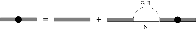
FIG. 1.: Dressing of a resonance propagator by $\pi$- and $\eta$-loops.

FIG. 2.: Diagrams of the contributions to the elementary Born amplitude: nucleon pole graph (NP), crossed nucleon pole graph (NC), pion pole graphs (PP), Z-graphs (Z), and vector meson exchange (VM).

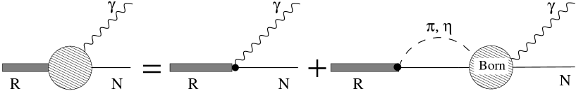
FIG. 3.: Dressing of the e.m. resonance vertex by rescattering.

FIG. 4.: Resonance contribution to the elementary meson photoproduction process including the dressed $\gamma NR$ vertex (see Fig. 3).

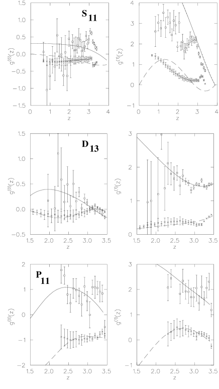
FIG. 5.: Effective e.m. coupling strength of the nucleon resonances extracted from the experimental multipoles [25]. Notation: $\Box$ real part of the effective couplings; $\times$ imaginary part of the effective couplings; full curves: fit of the parametrization of Eq. (20) to the real part; dashed curves: fit to the imaginary part.

FIG. 6.: Total cross section of $\eta$-photoproduction on the proton. Experimental data: $\Box$: Krusche et al. [17], $\times$: Wilhelm et al. [26].

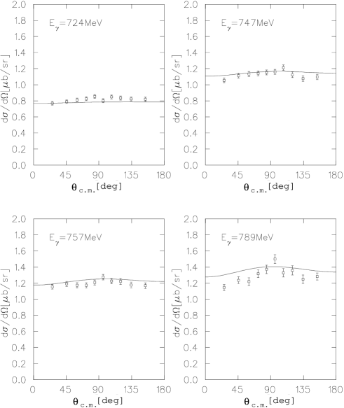
FIG. 7.: Differential cross section of $\eta$-photoproduction on the proton. Experimental data from [17]

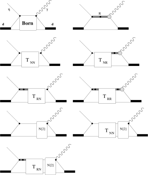
FIG. 8.: Diagrammatical overview of the model of coherent $\eta$-photoproduction on the deuteron. The box labeled Born contains also disconnected diagrams where the photon is absorbed by one nucleon and the $\eta$ is emitted by the other. Hadronic rescattering is indicated by the square boxes labeled $T_{NN}$, $T_{NR}$, $T_{RN}$, and $T_{RR}$. Meson exchange current contributions are indicated by the boxes labeled $N[2]$.

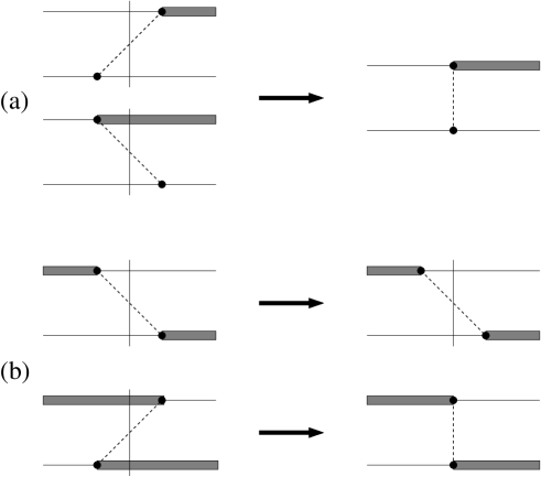
FIG. 9.: Treatment of the different time orderings of the hadronic transition potentials. (a) static approximation for the $NN\leftrightarrow{}NR$ potential, (b) upper part: retarded $NR$ exchange potential, lower part: static approximation of the meson-RR propagator.

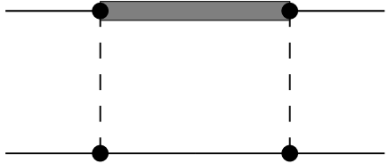
FIG. 10.: Static nucleon-resonance box used in the renormalization scheme of Green and Sainio.

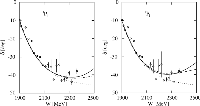
FIG. 11.: ${}^{1}P_{1}$-phase shift of $NN$-scattering as function of the invariant energy $W$ of the $NN$-system. Notation of curves: dotted: OBEPQ-B $NN$-potential, dash-dot: coupled channel with static rescattering and box renormalization, solid: coupled channel with retarded rescattering and box renormalization. Left panel: rescattering through $NS_{11}$ only, right panel: complete rescattering. The data are from the VPI analysis [25].

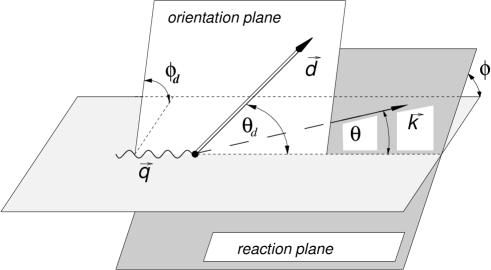
FIG. 12.: Kinematical variables of the coherent $\eta$-photoproduction process on the deuteron.

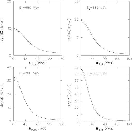
FIG. 13.: Differential cross section of $d(\gamma,\eta)d$ including the resonance graphs only. Notation of the curves: dotted: $S_{11}(1535)$, dashed: $S_{11}(1535)$ + $D_{13}(1520)$, full: $S_{11}(1535)$ + $D_{13}(1520)$ + $P_{11}(1440)$.

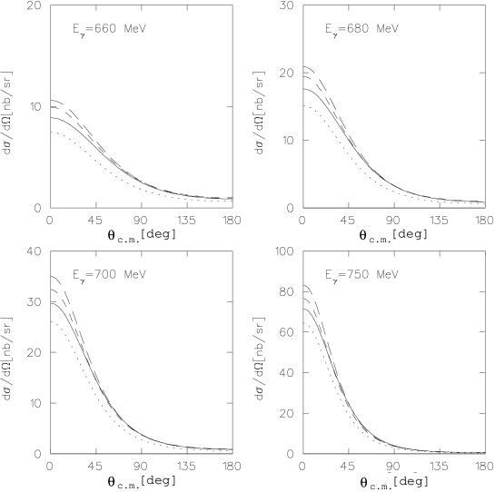
FIG. 14.: Effects of the Born terms on the differential cross section of $d(\gamma,\eta)d$. Notation of the curves: short-dashed: direct resonant graphs $S_{11}(1535)$ + $D_{13}(1520)$ + $P_{11}(1440)$, long-dashed: + direct and crossed nucleonic graphs, including the two unconnected graphs, dotted: + Z-graphs, full: + $\omega$-meson contribution = IA.

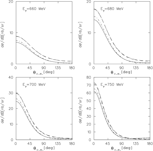
FIG. 15.: Effect of the different static rescattering mechanisms involving the $S_{11}$ resonance on the differential cross section of $d(\gamma,\eta)d$. Notation of the curves: short-dashed: IA, long-dashed: IA + static transition $NS_{11}\leftrightarrow{}NN$ rescattering, dash-dotted: IA + static $NS_{11}\leftrightarrow{}NS_{11}$ rescattering, full: IA + both $NS_{11}$ rescattering contributions.

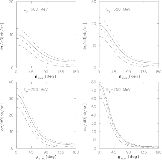
FIG. 16.: Effect of the different retarded rescattering mechanisms on the differential cross section of $d(\gamma,\eta)d$. Notation of the curves: short-dashed: IA, long-dashed: IA + $NN$ rescattering + static $NS_{11}$-rescattering, dash-dotted: IA + $NN$ rescattering + retarded $NS_{11}$-rescattering, full: IA + all retarded rescattering contributions, i.e., including the higher resonances but without MEC.

FIG. 17.: Effect of the retarded $\pi$- and $\eta$-exchange rescattering on the differential cross section of $d(\gamma,\eta)d$. Notation of the curves: short-dashed: IA, long-dashed: IA + $NN$ rescattering + retarded $\pi$-exchange $NS_{11}$ rescattering, dotted: IA + $NN$ rescattering + retarded $\eta$-exchange $NS_{11}$ rescattering, full: IA + $NN$ rescattering + both retarded $NS_{11}$ rescattering contributions.

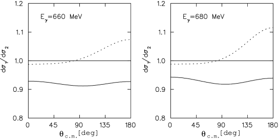
FIG. 18.: Relative effect of MEC operators on the differential cross section of $d(\gamma,\eta)d$. Notation of the curves: dotted: ratio of IA + static $\pi$- and $\eta$-MEC to IA, full: ratio of IA + all retarded rescattering mechanisms + MEC + $RNN[2]$- and $RS_{11}N[2]$-graphs to IA + all retarded rescattering mechanisms.

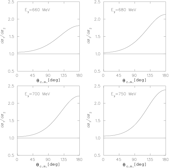
FIG. 19.: Relative effect of all two-body operators on the differential cross section of the coherent reaction. Notation of the curves: full: ratio of the complete calculation to IA.

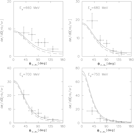
FIG. 20.: Summary of all contributions to the differential cross section of $d(\gamma,\eta)d$ and comparison to experiment. The data points are taken from [1]. Notation of the curves: dashed: IA, full: complete calculation, i.e., IA + MEC + retarded rescattering, including the combination of MEC and rescattering.

FIG. 21.: Total cross section of the coherent reaction $\gamma{}d\rightarrow\eta{}d$ for energies up to $E_{\gamma}^{lab}=850\;\mbox{MeV}$. Notation of the curves: dotted: pure resonance contribution, long-dashed: IA, short-dashed: IA + retarded first order rescattering, full: complete calculation, i.e., IA + all retarded rescattering contributions + MEC + RNN[2] + RXN[2].

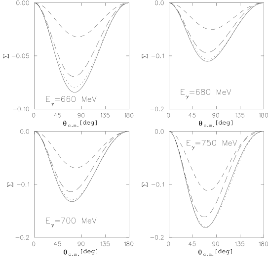
FIG. 22.: Linear photon asymmetry of $d(\gamma,\eta)d$ at various photon energies. Notation of the curves: short-dashed: pure resonant contribution, long-dashed: IA, dotted: IA + retarded rescattering, full: complete calculation.

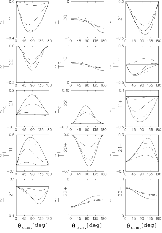
FIG. 23.: Target and beam-target polarization observables for $d(\gamma,\eta)d$ at $E_{\gamma}^{lab}=700\;\mbox{MeV}$. Notation of the curves as in Fig. 22.

REFERENCES

- [1] P. Hoffmann-Rothe et al., Phys. Rev. Lett. 78, 4697 (1997).
- [2] E. Breitmoser and H. Arenhövel, Nucl. Phys. A 612, 321 (1997).
- [3] N. Hoshi, H. Hyuga, and K. Kubodera, Nucl. Phys. A 324, 234 (1979).
- [4] R.L. Anderson and R. Prepost, Phys. Rev. Lett. 23, 46 (1969).
- [5] D. Halderson and A.S. Rosenthal, Nucl. Phys. A 501, 856 (1989).
- [6] S.S. Kamalov, L. Tiator, and C. Bennhold, Phys. Rev. C 55, 98 (1997).
- [7] A. Fix, private communication.
- [8] F. Ritz and H. Arenhövel, Phys. Lett. B 447, 15 (1999).
- [9] C. Bennhold and H. Tanabe, Nucl. Phys. A 530, 625 (1991).
- [10] M. Benmerrouche, N.C. Mukhopadhyay, and J.F. Zhang, Phys. Rev. D 51, 3237 (1995).
- [11] A.M. Green and S. Wycech, Phys. Rev. C 60, 035208 (1999).
- [12] L. Tiator, C. Bennhold, and S.S. Kamalov, Nucl. Phys. A 580, 455 (1994).
- [13] G. Knöchlein, D. Drechsel, L. Tiator, Z. Phys. A 352, 327 (1995).
- [14] H. Tanabe and K. Ohta, Phys. Rev. C 31, 1876 (1985).
- [15] Th. Wilbois, P. Wilhelm, and H. Arenhövel, Phys. Rev. C 57, 295 (1998).
- [16] P. Wilhelm, T. Wilbois, and H. Arenhövel, Phys. Rev. C 54, 1423 (1996).
- [17] B. Krusche et al., Phys. Rev. Lett. 74, 3736 (1995).
- [18] P. Wilhelm and H. Arenhövel, Nucl. Phys. A 593, 435 (1995).
- [19] F. Ritz, PhD thesis, Universität Mainz, 2000.
- [20] A.M. Green and M.E. Sainio, Journ. Phys. G 8, 1337 (1982).
- [21] H. Arenhövel, Few-Body Syst. 27, 141 (1999).
- [22] F. Blaazer, B.L.G. Bakker, and H.J. Boersma, Nucl. Phys. A590, 750 (1995).
- [23] R. Machleidt, K. Holinde, and Ch. Elster, Phys. Rep. 149, 1 (1987); R. Machleidt, Adv. Nucl. Phys. 19, 189 (1989).
- [24] A. Fix and H. Arenhövel, Z. Phys. A 359, 427 (1997).
- [25] R. Arndt et al., program “SAID”, URL http://said.phys.vt.edu, solution “SP97”.
- [26] M. Wilhelm, PhD thesis, Universität Bonn, 1993; B. Schoch et al., Proc. Part. Nucl. Phys. 34, 43 (1995).