Exact solution of the nuclear pairing problem

Abstract

In many applications to finite Fermi-systems, the pairing problem has to be treated exactly. We suggest a numerical method of exact solution based on SU(2) quasispin algebras and demonstrate its simplicity and practicality. We show that the treatment of binding energies with the use of the exact pairing and uncorrelated monopole contribution of other residual interactions can serve as an effective alternative to the full shell-model diagonalization in spherical nuclei. A self-consistent combination of the exactly treated pairing and Hartree-Fock method is discussed. Results for Sn isotopes indicate a good agreement with experimental data.

Pairing correlations play an essential role in nuclear structure properties including binding energies, odd-even effects, single-particle occupancies, excitation spectra, electromagnetic and beta-decay probabilities, transfer reaction amplitudes, low-lying collective modes, level densities, and moments of inertia [1, 2, 3]. The revival of interest in pairing correlations is related to studies of nuclei far from stability and predictions of exotic pairing modes [4, 5]. Metallic clusters, organic molecules and Fullerenes are other examples of finite Fermi systems with possibilities for pairing correlations of the superconducting type [6].

The conventional description of pairing usually employs the classical BCS approach [7] used in theory of superconductivity. This approximate solution has a very good accuracy for large systems and becomes exact in the asymptotic limit [8]. The shortcomings of the BCS approximation for small systems are well known, see for example [9] and references therein. The major drawback of the BCS is the violation of particle number conservation, which gives rise to deviations from the exact solution for small systems. Various ideas have been suggested to correct this deficiency, such as the number projection mean-field methods [10, 11, 12], coherent state approach [13], stochastic number projection [14], statistical descriptions [15], treatments of residual parts of the Hamiltonian in the random phase approximation [16, 17], and recurrence relation methods [18, 19]. These methods have found only a limited number of practical applications; for some approaches the obtained results did not manifest the desired accuracy whereas other methods are limited by practical complications. BCS-like approximate theories have a number of other deficiencies when applied to small systems [1, 9]. In particular, in the region of weak pairing the BCS has a sharp phase transition from the paired condensate to the normal state with no pairing (trivial or zero gap solution), whereas exact solutions exhibit the existence of exponentially decreasing pairing correlations all the way down to the zero pairing strength. This difficulty makes the BCS method unreliable for applications to weakly bound nuclei and calls for improvements and extensions such as BCS+RPA [20]. There are also serious problems related to the correct description of pairing in excited states.

The exact pairing (EP) method presented in this work allows one to solve exactly the general pairing Hamiltonian

$$H=\sum_{j\,m}\epsilon_{j}a^{\dagger}_{j\,m}a_{j\,m}\,+\,{1\over 4}\sum_{j,\,j^{\prime}}G_{j\,j^{\prime}}\,\sum_{m,\,m^{\prime}}\,a^{\dagger}_{j\,m}{\tilde{a}^{\dagger}_{j\,m}}{\tilde{a}_{j^{\prime}\,m^{\prime}}}a_{j^{\prime}\,m^{\prime}}\,,\quad{\tilde{a}_{j\,m}}\equiv(-1)^{j-m}a_{j\,-m}\,,$$ (1)

where $\{\epsilon_{j}\}$ is the set of single-particle energies, diagonal $G_{j\,j}$ are pairing energies, and $G_{j\,j^{\prime}}=G_{j^{\prime}\,j}$ for $j\neq j^{\prime}$ are pair transfer matrix elements, ($j^{\prime}\leftrightarrow j$). The practical usefulness of the EP algorithm comes from the facts that it is exact, fast and allows a straightforward extension for an approximate treatment of other components of residual interactions. Some realistic examples are presented in this work to emphasize these points. As a result, it becomes unnecessary to use complex approximate methods, such as BCS and all those associated with it, when exact results that are free of all problems discussed above can be obtained with an almost equal or even smaller effort.

A number of methods for treating the pairing problem exactly have been previously proposed. The Richardson method, described in the series of papers [21], provides a formally exact way for solving the pairing Hamiltonian. This method reduces the large-scale diagonalization of a many-body Hamiltonian in a truncated Hilbert space to a set of coupled equations with a dimension equal to the number of valence particles. Recently, exact solutions have been approached by introducing sophisticated mathematical tools such as infinite-dimensional algebras [22]. Such formally exact solutions have a certain merit from a mathematical point of view and for developing and understanding approximate calculations. However, due to their complexity they are not very useful in solving practical problems in nuclear physics.

The natural way of solving the pairing problem is related to the direct Fock-space diagonalization. For deformed nuclei with the doubly degenerate single-particle orbitals this approach supplemented by the appropriate use of symmetries and truncations was already shown to be quite effective [23, 24]. Our goal is to combine the exact treatment of pairing with the approximate inclusion of other parts of the residual interaction. Here the framework of the rotationally invariant shell model is the most convenient, especially because it allows us to fully utilize the well known ideas (see for example [25, 13]), based on the existence of quasispin symmetry in paired systems first studied in the 1940’s by Racah [26]. In the context of the shell model similar ideas were utilized in [27]. We use the quasispin algebra for each subset of degenerate single-particle levels. The fact that Racah’s degenerate model is analytically solvable comes purely from this algebraic feature. The spherical shell model with its m-degeneracies is a perfect arena for applying this method and therefore we will use notations associated with the case of spherical symmetry and j-j coupling. This certainly does not limit the generality of approach.

The Hamiltonian Eq. (1) can be rewritten as

$$H=\sum_{j}\,\epsilon_{j}\Omega_{j}+2\,\sum_{j}\,\epsilon_{j}L^{z}_{j}+\sum_{j\,j^{\prime}}\,G_{j\,j^{\prime}}L^{+}_{j}L^{-}_{j^{\prime}}\,,$$ (2)

by introducing the partial quasispin operators $L^{+}_{j}$, $L^{-}_{j}$ and $L^{z}_{j}$ for each $j$-level as follows

$$L^{-}_{j}=\frac{1}{2}\,\sum_{m}\,{\tilde{a}_{j\,m}}a_{j\,m}\,,\quad L^{+}_{j}=\left(L^{-}_{j}\right)^{\dagger}=\frac{1}{2}\,\sum_{m}\,a^{\dagger}_{j\,m}{\tilde{a}^{\dagger}_{j\,m}}\,,$$ (3)

$$L^{z}_{j}=\frac{1}{2}\,\sum_{m}\,\left(a^{\dagger}_{j\,m}a_{j\,m}-\frac{1}{2}\right)\,=\frac{1}{2}(N_{j}-\Omega_{j})\,,$$ (4)

where $N_{j}$ is the particle number operator and $\Omega_{j}=(2j+1)/2$ is the pair degeneracy of a given single-particle level $j\,.$ It can be shown directly from the definitions of $L^{+}_{J}$, $L^{-}_{j}$ and $L^{z}_{j}$ that they form an SU(2) algebra of angular momentum,

$$\left[L^{+}_{j},L^{-}_{j^{\prime}}\right]=2\delta_{j\,j^{\prime}}\,L^{z}_{j}\,,\,\,\left[L^{z}_{j},L^{+}_{j^{\prime}}\right]=\delta_{j\,j^{\prime}}\,L^{+}_{j}\,,\,\,\left[L^{z}_{j},L^{-}_{j^{\prime}}\right]=-\delta_{j\,j^{\prime}}\,L^{-}_{j}\,.$$ (5)

Expressed in terms of quasispins, the Hamiltonian in (2) makes the pairing problem equivalent to the problem of interacting spins in a magnetic field, a generalized form of the Zeeman effect [28]. It is clear that every square of the partial quasispin ${\bf L}_{j}^{2}=L^{+}_{j}L^{-}_{j}-L^{z}_{j}+(L^{z}_{j})^{2}$ commutes with the Hamiltonian making $L_{j}$, corresponding to the eigenvalue $L_{j}(L_{j}+1)$ of ${\bf L}_{j}^{2}$, a good quantum number in the pairing problem. This brings in the major simplification of the problem. The maximum value that $L_{j}$ can take is $\Omega_{j}/2\,,$ which happens for a fully paired subshell, such as, for example, the completely occupied subshell case where $N_{j}=2\Omega_{j}$, $L^{z}_{j}=L_{j}=\Omega_{j}/2\,.$ Lower values of the quasispin quantum number correspond to the Pauli blocking of a part of the pair space $\Omega_{j}$ by $s_{j}$ unpaired particles. This reduces the allowed space to $\Omega_{j}-s_{j}\,.$ The number $s_{j}$ can be called the seniority of a given $j$-shell. Being related to the quasispin, $s_{j}$ are conserved by the pairing interaction (2). Introducing the partial seniority $s_{j}$ and partial occupancy $N_{j}$ by means of

$$L_{j}=\frac{1}{2}(\Omega_{j}-s_{j})\,\quad L_{j}^{z}=\frac{1}{2}(N_{j}-\Omega)\,,$$ (6)

we will use $|s_{j},N_{j}\rangle$ instead of the SU(2) notation $|L_{j},L_{j}^{z}\rangle\,.$

The quasispin projections $L^{z}_{j}\,,$ or the partial occupancies $N_{j}\,,$ are not conserved because of the pair transfer term $G_{j\,j^{\prime}}$ (pair vibration). The usual constraints on angular momentum $0\leq|L_{j}^{z}|\leq L_{j}$ lead to $s_{j}\leq N_{j}\leq 2\Omega_{j}-s_{j}$ and $s_{j}\leq\Omega_{j}$ that have obvious interpretations. Furthermore, since both $L_{j}$ and $L_{j}^{z}$ must be simultaneously either integers or half-integers, $s_{j}$ is of the same parity as $N_{j}\,,$ confirming that particles are transfered only in pairs. Finally, there is a given total number of particles in the system $N=\sum_{j}\,N_{j}\,,$ and one can introduce the total seniority $s=\sum_{j}\,s_{j}\,.$ Both quantities are conserved by the Hamiltonian and must be of the same parity.

For each representation given by the set of quantum numbers $\{s_{j}\}\,,$ one can construct basis states $|\{s_{j}\},\,\{N_{j}\}\rangle$ going through all permutations of $N$ fermions allowed by above constraints. Finally, a Hamiltonian matrix can be constructed in this basis using standard properties of the angular momentum operators

$$L^{\pm}|L,\,L_{z}\rangle=\sqrt{(L\mp L_{z})(L\pm L_{z}+1)}\,|L,\,L\pm 1\rangle\,.$$ (7)

Diagonal elements become

$$\langle\{s_{j}\},\,\{N_{j}\}|H|\{s_{j}\},\,\{N_{j}\}\rangle=\sum_{j}\left(\epsilon_{j}N_{j}+\frac{G_{j\,j}}{4}(N_{j}-s_{j})(2\Omega_{j}-s_{j}-N_{j}+2)\right)\,,$$ (8)

and off-diagonal elements that transfer pairs are

$$\langle\{s_{j}\},\,\dots N_{j}+2,\dots N_{j^{\prime}}-2,\dots|H|\{s_{j}\},\,\dots N_{j},\cdots N_{j^{\prime}},\dots\rangle$$

$$=\frac{G_{j\,j^{\prime}}}{4}\sqrt{(N_{j^{\prime}}-s_{j^{\prime}})(2\Omega_{j^{\prime}}-s_{j^{\prime}}-N_{j^{\prime}}+2)(2\Omega_{j}-s_{j}-N_{j})(N_{j}-s_{j}+2)}\,.$$ (9)

Diagonalization of this matrix for each representation, a given set of partial seniorities $\{s_{j}\}\,,$ is the final step in the solution. The largest Hamiltonian matrix in partial seniority basis, which corresponds to the lowest allowed total seniority, has a dimension much lower than the total fermionic many-body space. Even for the set of valence orbits encountered in heavy nuclei it does not exceed several thousands. As seen from the above discussion, the Hamiltonian matrix is very sparse.

Each state of a non-zero seniority is degenerate since $s_{j}$ unpaired particles are untouched by the Hamiltonian and are free to move within a given $j$-shell, provided that they all remain unpaired. The number of these fermionic degrees of freedom for each $j$ is $C(2\Omega_{j},s_{j})-C(2\Omega_{j},s_{j}-2)$ where $C(m,n)=m!/(n!(m-n)!)$ is a binomial coefficient. The total degeneracy of each state in the $\{s_{j}\}$ seniority class is

$$\prod_{j}\,\left[C(2\Omega_{j},s_{j})-C(2\Omega_{j},s_{j}-2)\right]\,.$$ (10)

The resulting degenerate states that carry seniority quantum numbers can be further classified according to other symmetry groups of the Hamiltonian such as angular momentum. All total seniority zero states have spin zero. For non-zero seniorities, one first has to determine allowed angular momenta for a given subshell $j$ with $s_{j}$ unpaired particles and then make all possible couplings of subshells to a total spin.

To illustrate the practical application of this algorithm, we show below examples involving chains of Ca and Sn isotopes. The Ca isotopes occupy the fp shell with the model space consisting of four levels $f_{7/2},\,p_{3/2},\,f_{5/2},$ and $p_{1/2}\,.$ This amounts to a total neutron capacity of 20. The pair transfer matrix elements are taken from the FPD6 interaction [29]. The results in Fig. 1(b) are obtained with single-particle energies appropriate for the above-mentioned $j$-levels in ⁴⁸Ca: -9.9, -5.1, -1.6, and -3.1 MeV, respectively. Fig. 1(b) shows the correlation energies in the Ca isotopes, defined as

$$E_{\rm corr}=E-\sum_{j}\epsilon_{j}\bar{N_{j}}-\sum_{j}\frac{G_{j\,j}}{2\Omega_{j}-1}\,\frac{\bar{N_{j}}(\bar{N_{j}}-1)}{2}\,,$$ (11)

where $E$ is the energy of the ground state and $\bar{N_{j}}$ is the (noninteger) expectation value of the ground state occupancy of the $j$-level, found as a result of the EP calculation. It is known [1] that in a system with a discrete single-particle spectrum the nontrivial BCS solution exists only at a sufficiently strong pairing interaction which can overcome the single-particle level spacings. In contrast to that, in macroscopic Fermi-systems the nontrivial Cooper phenomenon exists at any strength of the attractive pairing interaction. The fact of inadequacy of the BCS approximation for weak pairing was pointed out by many authors, for example [9, 24]. Near the ⁴⁸Ca shell closure there is a 4.8 MeV gap between $f_{7/2}$ and higher single-particle orbitals, and as it can be seen from Fig. 1(b), BCS can no longer support the pairing condensate. It gives instead a normal Fermi-gas solution with zero pairing energy, whereas in reality the EP solution demonstrates significant pairing effects with almost 2 MeV condensation energy.

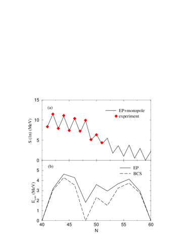
FIG. 1.: Panel (a): neutron separation energies in Ca isotopes, EP+monopole treatment of other interactions is compared with experimental points (diamonds); panel (b): pairing correlation energy in even-even Ca isotopes, the exact EP calculation (solid line) is compared with the standard BCS (dashed line).

In most of the real cases the pure pairing interaction ($J=0,\,T=1\,$) is strongly modified by residual interactions in other channels. A significant part of the remaining correlations in spherical nuclei can be treated by including only monopole (diagonal) part

$$\sum_{j}\bar{V}_{j\,j}\frac{N_{j}(N_{j}-1)}{2}+\sum_{j\neq j^{\prime}}\bar{V}_{j\,j^{\prime}}N_{j}N_{j^{\prime}}\,,$$ (12)

where

$$\bar{V}_{j\,j^{\prime}}=\frac{1+\delta_{j\,j^{\prime}}}{2\Omega_{j}(2\Omega_{j^{\prime}}-\delta_{j\,j^{\prime}})}\sum_{J\neq 0}(2J+1)\langle J;\,j\,j^{\prime}|V|J;\,j\,j^{\prime}\rangle\,$$ (13)

is the monopole-monopole part of the total interaction $V$ written in eq. (13) in terms of the diagonal matrix elements for the pairs $[jj^{\prime}]_{J}$. Pairing $\langle J=0;\,j\,j|V|J=0;\,j^{\prime}\,j^{\prime}\rangle=G_{j\,j^{\prime}}\sqrt{\Omega_{j}\Omega_{j^{\prime}}}\,$ is not included in the sum since it is treated exactly by EP and its monopole term is present in Eq. (8). One-neutron separation energies shown in Fig. 1(a) were calculated with this EP plus monopole method, using the FPD6 interaction and single-particle energies for ⁴¹Ca. These results agree very well with experimentally observed separation energies, shown on the figure with diamonds. Ground state energies, obtained with this method for Ca isotopes differ from those from the exact shell model diagonalization, using the total FPD6 [29] interaction, by less than 0.5 MeV; certainly the EP plus monopole results are exact for full and empty shells and for one-particle or one-hole cases.

For the second example of application we show in Fig. 2(b) the results for the Sn isotopes. The model space here consists of five single-particle levels $h_{11/2},\,d_{3/2},\,s_{1/2},\,g_{7/2},\,$ and $d_{5/2}\,,$ which can accommodate up to 32 neutrons. We will be interested in the evolution of neutron separation and correlation energies along the chain of the isotpes rather than in the specific spectra which were studied earlier with a number of approximate methods, for example [31], and can be considered in the future with our exact approach. The pairing matrix elements were obtained from the $G$-matrix derived from the recent CD-Bonn [32] nucleon-nucleon interaction with ¹³²Sn as a closed shell, where the $\hat{Q}$-box method includes all non-folded diagrams up to the third order in the interaction and sums up the folded diagrams to infinite order [33]. The most complex case is ¹¹⁶Sn (half-filled shell) with 601,080,390 many-body states of which 272,828 are of spin zero, so that even with the use of the angular momentum projection the problem remains difficult for direct diagonalization. There are only 420 independent seniority sets in the seniority basis. The largest matrix, $s=0\,,$ has a dimension of $110\,,$ the diagonalization of which is a trivial problem. Solution of the pairing problem for ¹¹⁶Sn with the algorithm discussed above is therefore simple and extremely fast.

The correlation energies obtained with the above $G$-matrix and single-hole energies -9.76, -8.98, -7.33, -7.66, and -7.57 MeV, based on the data for the ¹³¹Sn isotope [30], are shown in Fig. 2(b). A reduction of pairing also happens between $g_{7/2},\,d_{5/2}$ and the rest of the single-particle orbitals $h_{11/2},\,d_{3/2},\,s_{1/2}\,,$ but here BCS is just weakened which results only in relatively small suppression of correlation energy. A related application of EP is shown in Fig. 2(a) where one-neutron separation energies are calculated for the Sn isotopes, including those beyond ¹³²Sn. These energies were obtained from the fully self-consistent spherically symmetric solution of Hartree-Fock (HF) equations, using the SKX interaction [34], with the EP solution based on the above $G$-matrix at each HF iteration. The HF+EP method works as follows. An initial guess for the HF potential is used to obtain a set of spherical single-particle energies and densities for all of the occupied and valence orbitals. The single-particle enegies for the valence space plus a fixed set of two-body matrix elements are used in the EP method to obtain the pairing correlation energy and the valence single-particle occupation numbers. The initial set of single-particle densities plus the pairing occupation factors are used to obtain a new potential with the Skyrme hamiltonian. This proceedure is iterated until convergence (typically 60 iterations). The total energy is the sum of the Skyrme HF energy and the pairing correlation energy Eq. (11). The plot 2(a) exhibits an odd-even staggering that can only be attributed to pairing. The agreement between experiment and theory is excellent given that no parameters have been adjusted for these particular data.

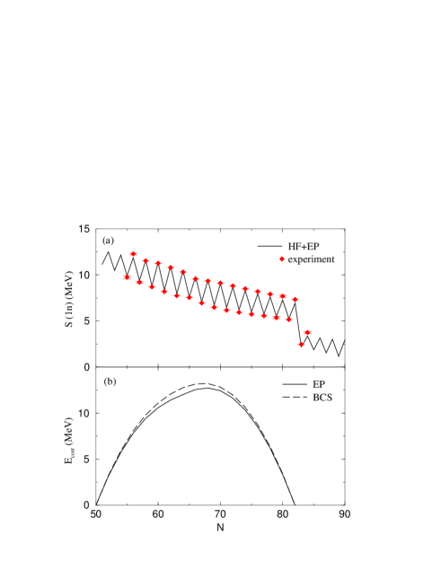
FIG. 2.: Panel (a): neutron separation energies calculated for the Sn isotopes using the self-consistent solution of Hartree-Fock plus Exact Pairing. Experimental points are shown for comparison. Panel (b): pairing correlation energy in even-even Sn isotopes, EP (solid line) and BCS (dashed line).

The EP algorithm presented here in our view has a good future as a tool for different calculations related to pairing. It is exact, fast and reliable which makes it perfect for pure shell model calculations with pairing, fast estimates of binding energies and spectroscopic factors, for the use as a basis for treatment of other interactions, iterative HF calculations and many other tasks.

This work was supported by the National Science Foundation, grants No. 9605207 and 0070911. The schematic model was studied with E. Keller in the framework of the REU program at MSU [35]. The authors thank S. Pratt for motivating discussions and G. Bertsch, A. Klein, M. Mostovoy, and D. Mulhall for useful comments. M. Hjorth-Jensen kindly provided the renormalized $G$-matrix for the ¹³²Sn region.

REFERENCES

- [1] S.T. Belyaev, Mat. Fys. Medd. Dan. Vid. Selsk. 31, No. 11 (1959); in Selected Topics in Nuclear Theory, ed. F. Janouch (IAEA, Vienna, 1963) p. 291.
- [2] A. Bohr and B. Mottelson, Nuclear Structure, Vol. 2 (Benjamin, New York, 1974).
- [3] M. Hasegawa, S. Tazaki, Phys. Rev. C 47, 188 (1993).
- [4] A.L. Goodman, Adv. Nucl. Phys. 11, 263 (1979).
- [5] R.A. Broglia, J. Terasaki, N. Giovanardi, Phys. Rep. 335, 1 (2000).
- [6] M. Barranco, S. Hernandez and R.M. Lombard, Z. Phys. D 22, 659 (1992).
- [7] J. Bardeen, L.N. Cooper and J.R. Schrieffer, Phys. Rev. 108, 1175 (1957).
- [8] N.N. Bogoliubov, JETP 34, 58 (1958); Physica 26, 1 (1960).
- [9] P. Ring and P. Schuck, The Nuclear Many-Body Problem, (Springer-Verlag, New York, 1980).
- [10] H. J. Lipkin, Ann. Phys. 31, 528 (1960).
- [11] Y. Nogami, Phys. Rev. 134B, 313 (1964); Y. Nogami, I. J. Zucker, Nucl Phys. 60, 203 (1964).
- [12] W. Satula and R. Wyss, Nucl. Phys. A 676, 120 (2000).
- [13] H. Chen, T. Song and D.J. Rowe, Nucl. Phys. A582, 181 (1995).
- [14] R. Capote and A. Gonzalez, Phys. Rev. C 59, 3477 (1999).
- [15] S. Das Gupta and N. De Takacsy, Nucl. Phys. A240, 293 (1975).
- [16] J. Bang and J. Krumlinde, Nucl. Phys. A141, 18 (1970).
- [17] O. Johns, Nucl. Phys. A154, 65 (1970).
- [18] G. Do Dang and A. Klein, Phys. Rev. 143, 735 (1966).
- [19] F. Andreozzi, A. Covello, A. Gargano, Liu Jian Ye, and A. Porrino, Phys. Rev. C 32 293, (1985).
- [20] K. Hagino and G.F. Bertsch, Nucl. Phys. A. 679, 163 (2000).
- [21] R. W. Richardson, Phys. Lett. 3, 277 (1963); 5, 82 (1963); 14, 325 (1965).
- [22] Feng Pan, J. P. Draayer, W. E. Ormand, Phys. Lett. B 422, 1 (1998).
- [23] O. Burglin and N. Rowley, Nucl. Phys A 602, 21 (1996).
- [24] H. Molique and J. Dudek, Phys. Rev. C 56, 1795 (1997).
- [25] A. K. Kerman, R. D. Lawson, and M. H. Macfarlane, Phys. Rev. 124, 162 (1961).
- [26] G. Racah, Phys. Rev. 62, 438 (1942); Phys. Rev. 63, 367 (1943).
- [27] N. Auerbach, Nycl. Phys. 76, 321 (1966).
- [28] A.M. Lane, Nuclear Theory (Benjamin, New York, 1964).
- [29] W. A. Richter, M. G. van der Merwe, R. E. Julies and B. A. Brown, Nucl. Phys. A523, 325 (1991).
- [30] R.B. Firestone, V.S. Shirley, C.M. Baglin, S.Y. Frank Chu and J. Zipkin, Table of Isotopes (1996).
- [31] F. Andreozzi, L. Coraggio, A. Covello, A. Gargano, A. Porrino, Z. Phys. A 345, 253 (1996).
- [32] R. Machleidt, F. Sammarruca and Y. Song, Phys. Rev. C 53, R1483 (1996).
- [33] M. Hjorth-Jensen, T.T.S. Kuo and E. Osnes, Phys. Rep. 261, 125 (1995); M. Hjorth-Jensen, H. Muther, E. Osnes and A. Polls, J. Phys. 22, 321 (1996).
- [34] B. A. Brown, Phys. Rev. C 58, 220 (1998).
- [35] E. Keller, V. Zelevinsky, and A. Volya, BAPS 45 No. 5, 23 (2000).