Calculations of three-body observables in ⁸B breakup

Abstract

We discuss calculations of three-body observables for the breakup of ⁸B on a ⁵⁸Ni target at low energy using the coupled discretised continuum channels approach. Calculations of both the angular distribution of the ⁷Be fragments and their energy distributions are compared with those measured at several laboratory angles. In these observables there is interference between the breakup amplitudes from different spin-parity excitations of the projectile. The resulting angle and the energy distributions reveal the importance of the higher-order continuum state couplings for an understanding of the measurements.

I Introduction

Projectile breakup is an important reaction channel in the scattering of weakly bound nuclei. An accurate treatment of breakup is therefore a major ingredient in attempts to understand the properties of light exotic radioactive nuclei from reaction studies. The number of published experimental breakup studies, and also their accuracy, has increased rapidly. These include reactions in which both nuclear and Coulomb breakup effects are expected to be significant, e.g. [1, 2, 3, 4, 5, 6, 7, 8, 9, 10, 11, 12, 13, 14, 15, 16, 17]. Until recently, the low intensities of available rare isotope beams has meant that many of the experiments were either designed to measure inclusive cross sections, with incomplete kinematics, or did not have adequate statistics to allow the extraction of exclusive observables. The cross sections extracted from the measurements were often integrated over fragment energies or angles, or both, and inevitably some details of the physical process were lost as a result. This is no longer the situation. Secondary beam intensities are becoming sufficiently high that coincidence experiments are now practical and, in the future, data will more routinely require a fully three- or more-body study, e.g. [18, 19]. The need for precise theoretical predictions of the breakup of two-body projectiles, and of their three-body observables, is the primary motivation for this work.

Theoretical reaction models, which treat breakup as an excitation of the projectile to a two-body continuum state, most naturally express their results as cross sections describing the center of mass (c.m.) and relative motions of the dissociated system, using 2-body kinematics. It has therefore been common for the experimental data to also be transformed to the c.m. frame, for ease of comparison, e.g. the theoretical calculations of [20, 21] and the experimental data of [17]. This process is ambiguous in the case of inclusive data. Much more important is that the three-body cross sections are explicitly coherent in contributions from different spin-parity excitations of the projectile and so have the potential to offer a far greater insight into the projectile structure and the reaction mechanism. An excellent example of this is the interference observed [14] in the cross section of the ⁷Be fragments, as a function of their component of momentum parallel to the beam direction, following ⁸B breakup on a heavy target at 44 MeV/nucleon.

In this paper we present calculations which are performed using full three-body kinematics. These calculations are carried out within the framework of the coupled discretised continuum channels (CDCC) methodology, e.g. [22, 23], for breakup reactions of two-body projectiles. The interference between different excitation channels is shown to be significant for assessing the convergence of the calculations and those breakup excitations which contribute. The methods presented are applied to the breakup of ⁸B on a ⁵⁸Ni target at $E_{lab}=25.8$ MeV, for which new measurements have been reported [17, 24]. We compare the results of the full CDCC analysis, and also distorted waves Born approximation (DWBA) and truncated coupled channels calculations, with these available data for the laboratory angle and energy distributions of the ⁷Be fragments. The calculations of Refs. [20, 21] showed the importance of higher-order breakup couplings, the couplings between continuum states, upon the ⁸B^∗ center of mass cross section angular distribution. We will show in this work that these higher-order effects are manifest even more significantly in the energy distributions of the ⁷Be fragments following breakup.

II Theoretical Considerations

We consider the breakup reaction $p\rightarrow c+v$ in which the projectile nucleus $p$ is a bound state of a core particle $c$, of spin $I$ and projection $\mu$, and a valence particle $v$, of spin $s$ and projection $\sigma$. These particles are, presently, assumed structureless and so their internal wave functions are represented by the spinors ${\cal X}_{I}$ and ${\cal X}_{s}$. The total angular momentum of the ground state of $p$ is $J_{p}$, with projection $M$, the relative orbital angular momentum of the two constituents is $\ell_{0}$, and their separation energy is ${\cal E}_{0}\ (>0)$. The incident wave number of the projectile in the center of mass (c.m.) frame of the projectile and target is $\vec{K}_{0}$ and the co-ordinate $z$–axis is chosen in the incident beam direction. The target $t$ is assumed to have spin zero and no explicit target excitation is included. Target excitation is therefore present only through the complex effective interactions of $c$ and $v$ with the target. Our three-body solution of the Schrödinger equation calculates an approximate description of the projection of the full many-body $p+t$ wave function onto the ground states of the target, core and valence nuclei. This three-body wave function is denoted $\Psi_{\vec{K}_{0}M}(\vec{r},\vec{R})$ where $\vec{R}$ is the position of the c.m. of $p$ relative to the target and $\vec{r}$ is the position of $v$ relative to the core $c$. The particle masses are $m_{p}=m_{c}+m_{v}$ and $m_{t}$.

A Construction of continuum bin states

In the coupled discretised continuum channels (CDCC) method [22, 23] the breakup of $p$ is assumed to populate a finite set of selected $c+v$ excited configurations, with quantum numbers $J_{p}^{\prime},\ell,j$, where $\vec{j}=\vec{\ell}+\vec{s}$ and $\vec{J}_{p}^{\prime}=\vec{j}+\vec{I}$. Here, each of these spin-parity excitations will be assumed diagonal in all of these angular momentum labels. The excitations are also assumed to extend to some maximum relative energy ${\cal E}_{max}(J_{p}^{\prime})$ or wave number $k_{max}$. This momentum range is then divided into a number ${\cal N}(J_{p}^{\prime})$ of intervals or bins, each with a width $\Delta k_{i}=[k_{i}-k_{i-1}]$. We label each such momentum bin by $\alpha\equiv(i,J_{p}^{\prime},\ell,j,s,I)$.

In each of these relative motion bins a single representative wave function is constructed from those $c+v$ scattering states $f_{\alpha}(k,r)$ internal to the bin, with assumed angular momentum coupling

$$\hat{\phi}_{\alpha}^{M^{\prime}}(\vec{r})=\left[\left[Y_{\ell}(\hat{\vec{r}})\otimes{\cal X}_{s}\right]_{j}\otimes{\cal X}_{I}\right]_{J_{p}^{\prime}M^{\prime}}\,u_{\alpha}(r)/r~{}~{}.$$ (1)

The radial functions $u_{\alpha}$ are square integrable and are a superposition

$$u_{\alpha}(r)=\sqrt{\frac{2}{\pi N_{\alpha}}}\int_{k_{i-1}}^{k_{i}}g_{\alpha}(k)f_{\alpha}(k,r)\,dk~{}~{}$$ (2)

of the scattering states, eigenstates of the $c+v$ internal Hamiltonian $H_{p}$, with weight function $g_{\alpha}(k)$. $N_{\alpha}=\int_{k_{i-1}}^{k_{i}}|g_{\alpha}(k)|^{2}\,dk$ is a normalisation constant. The $f_{\alpha}$ are defined here such that, for $r\rightarrow\infty$,

$$f_{\alpha}(k,r)\rightarrow\left[\cos\delta_{\alpha}(k)F_{\ell}(kr)+\sin\delta_{\alpha}(k)G_{\ell}(kr)\right]~{},$$ (3)

where $k\in\alpha$ and $F_{\ell}$ and $G_{\ell}$ are the regular and irregular partial wave Coulomb functions. So the $f_{\alpha}$ are real when using a real $c+v$ two-body interaction. An optimal discretisation of the continuum requires a consideration of the number, the boundaries $k_{i}$, the widths $\Delta k_{i}$ and the weights $g_{\alpha}$ in the bins, which may depend on the $J_{p}^{\prime}$ configuration. Energy conservation relates the $c+v$ c.m. wave numbers $K_{\alpha}$ and corresponding bin state energies $\hat{{\cal E}}_{\alpha}$, as

$$\frac{\hbar^{2}K_{\alpha}^{2}}{2\mu_{pt}}+\hat{{\cal E}}_{\alpha}=\frac{\hbar^{2}K_{0}^{2}}{2\mu_{pt}}-{\cal E}_{0}~{},$$ (4)

where we define each bin energy by $\hat{{\cal E}}_{\alpha}=\langle\hat{\phi}_{\alpha}|H_{p}|\hat{\phi}_{\alpha}\rangle$ and where $\mu_{pt}$ is the projectile-target reduced mass.

For non-$s$-wave bins typically one uses $g_{\alpha}(k)=1$ for a non-resonant continuum in which case $N_{i}={\Delta k_{i}}$ and $\hat{{\cal E}}_{i}=\hbar^{2}\hat{k}_{i}^{2}/(2\mu_{cv})$ with $\hat{k}_{i}^{2}=[k_{i}^{3}-k_{i-1}^{3}]/(3\Delta k_{i})$. For $s$-wave bins it is an advantage to use $g_{\alpha}(k)=k$. This stabilises the extraction of the three-body transition amplitude at low relative breakup energies, discussed later in Eq. (15). In this case $N_{i}=\hat{k}_{i}^{2}{\Delta k_{i}}$ and the bin energies are $\hat{{\cal E}}_{i}=\hbar^{2}[k_{i}^{5}-k_{i-1}^{5}]/(10\mu_{cv}\Delta k_{i}\hat{k}_{i}^{2})$.

B Coupled channels amplitudes

These bin states $\hat{\phi}_{\alpha}$ provide an orthonormal relative motion basis for the coupled channels solution of the three-body $c+v+t$ wave function. The bins and the coupling potentials $\langle\hat{\phi}_{\alpha}|U(\vec{r},\vec{R})|\hat{\phi}_{\beta}\rangle$ are constructed, and the coupled equations are solved, using the coupled channels code fresco [25]. Here $U(\vec{r},\vec{R})$ is the sum of the interactions of $c$ and $v$ with the target, which is expanded to a maximum specified multipole order $q$. The coupled equations solution generates the (two-body) scattering amplitudes, summed over partial waves, for populating each bin state $J_{p}^{\prime},M^{\prime}$ from initial state $J_{p},M$, as a function of the angle $\theta_{K}$ of the c.m. of the excited projectile in the c.m. frame

$$\widehat{\cal F}_{M^{\prime}M}(\vec{K}_{\alpha}) = \frac{4\pi}{K_{0}}\,\sqrt{\frac{{K}_{\alpha}}{K_{0}}}\,\sum_{LL^{\prime}J}(L0J_{p}M|JM)\,(L^{\prime}M-M^{\prime}J_{p}^{\prime}M^{\prime}|JM)$$ (5)

$$\times \exp(i[\sigma_{L}+\sigma_{L^{\prime}}])\,\frac{1}{2i}\,\widehat{\cal S}^{J}_{LJ_{p}:L^{\prime}J_{p}^{\prime}}(K_{\alpha})\,Y_{L}^{0}(\widehat{\vec{K}}_{0})\,Y_{L^{\prime}}^{M-M^{\prime}}(\widehat{\vec{K}}_{\alpha})~{}~{}.$$ (6)

Here $\sigma_{L}$ and $\sigma_{L^{\prime}}$ are the Coulomb phases appropriate to the initial and final state c.m. energies and the $\widehat{\cal S}_{LJ_{p}:L^{\prime}J_{p}^{\prime}}(K_{\alpha})$ are the partial wave $S$–matrices for exciting bin state $\alpha$ with c.m. wave number $K_{\alpha}$. When calculated using fresco [25], these amplitudes are expressed in a coordinate system with $x$–axis in the plane of $\vec{K}_{0}$ and $\vec{K}_{\alpha}$, such that the azimuthal angle $\phi_{{K}_{\alpha}}$ of $\vec{K}_{\alpha}$ is zero. When discussing three-body observables, it is more convenient to define the coordinate system with respect to the fixed positions of the detectors in the laboratory. For such a general $x$–coordinate axis the coupled channels amplitudes must subsequently be multiplied by $\exp(i[M-M^{\prime}]\phi_{{K}})$, with $\phi_{K}$ referred to the chosen $x$-axis.

For use in the following, the two-body inelastic amplitudes of Eq. (6) are re-normalised to that of the $T$-matrix by removal of their two-body phase space factors, so that

$$\widehat{\cal T}_{M^{\prime}M}^{\alpha}(\vec{K}_{\alpha})=-\frac{2\pi\hbar^{2}}{\mu_{pt}}\,\sqrt{\frac{K_{0}}{K_{\alpha}}}\,\widehat{\cal F}_{M^{\prime}M}(\vec{K}_{\alpha})~{}~{}.$$ (7)

Throughout, we adopt scattering state and $T$-matrix normalisations such that, asymptotically, the plane wave states $\exp(i\vec{k}\cdot\vec{r})$ that enter are multiplied by unity.

It follows that the inelastic differential cross section angular distribution, in the center of mass frame, for excitation of a given bin state is

$$\frac{d\sigma(\alpha)}{d\Omega_{K}} = \frac{1}{2J_{p}+1}\,\left[\frac{\mu_{pt}}{2\pi\hbar^{2}}\right]^{2}\,\frac{K_{\alpha}}{K_{0}}\sum_{MM^{\prime}}\left|\widehat{\cal T}_{M^{\prime}M}^{\alpha}(\vec{K}_{\alpha})\right|^{2}$$ (8)

$$= \frac{1}{2J_{p}+1}\,\sum_{MM^{\prime}}\left|\widehat{\cal F}_{M^{\prime}M}(\vec{K}_{\alpha})\right|^{2}~{}~{}.$$ (9)

C Three-body breakup amplitudes

Less obvious is the relationship of the CDCC two-body inelastic amplitudes $\widehat{\cal T}_{M^{\prime}M}^{\alpha}(\vec{K}_{\alpha})$ to the breakup transition amplitudes $T_{\mu\sigma:M}(\vec{k},\vec{K})$ from an initial state $J_{p},M$ to a general physical three-body final state of the constituents [22, 26]. This is needed to make predictions for experiments with general detection geometries, since each detector configuration and detected fragment energy involves a distinct final state c.m. wave vector $\vec{K}$, breakup energy ${\cal E}_{k}$, and relative motion wave vector $\vec{k}$.

To clarify this connection we make the CDCC approximation to the exact (prior form) breakup transition amplitude, by replacing the exact $c+v+t$ three-body wave function, $\Psi_{\vec{K}_{0}M}(\vec{r},\vec{R})$, by its CDCC approximation $\Psi^{CD}$, as

$$T_{\mu\sigma:M}(\vec{k},\vec{K})=\langle\phi_{\vec{k}\mu\sigma}^{(-)}(\vec{r})\,e^{i\vec{K}\cdot\vec{R}}|U(\vec{r},\vec{R})|\Psi_{\vec{K}_{0}M}^{CD}(\vec{r},\vec{R})\rangle~{}~{}.$$ (10)

Here $\phi_{\vec{k}\mu\sigma}$ is the $c+v$ final state. Upon inserting the set of all included bin-states, which are assumed complete within the model space used, then

$$T_{\mu\sigma:M}(\vec{k},\vec{K})=\sum_{\alpha,M^{\prime}}\langle\phi_{\vec{k}\mu\sigma}^{(-)}|\hat{\phi}^{M^{\prime}}_{\alpha}\rangle\langle\hat{\phi}^{M^{\prime}}_{\alpha}\,e^{i\vec{K}\cdot\vec{R}}|U(\vec{r},\vec{R})|\Psi_{\vec{K}_{0}M}^{CD}(\vec{r},\vec{R})\rangle~{},$$ (11)

where the sum is over all bins $\alpha$ which contain wave number $k$. We should now recognise that the matrix elements $\widehat{\cal T}_{M^{\prime}M}^{\alpha}(\vec{K}_{\alpha})$ of Eq. (7), obtained from the coupled channels solution, are precisely the transition matrix elements appearing in Eq. (11), i.e.

$$\widehat{\cal T}_{M^{\prime}M}^{\alpha}(\vec{K}_{\alpha})=\langle\hat{\phi}^{M^{\prime}}_{\alpha}\,e^{i\vec{K}_{\alpha}\cdot\vec{R}}|U(\vec{r},\vec{R})|\Psi_{\vec{K}_{0}M}^{CD}(\vec{r},\vec{R})\rangle,$$ (12)

but calculated on the grid of $\theta_{\alpha}$ and $K_{\alpha}$ values. For the first term in Eq. (11) one obtains

$$\langle\phi_{\vec{k}\mu\sigma}^{(-)}|\hat{\phi}^{M^{\prime}}_{\alpha}\rangle=\frac{(2\pi)^{3/2}}{k\sqrt{N_{\alpha}}}\sum_{\nu}\,(-i)^{\ell}\,(\ell\nu s\sigma|jm)\,(jmI\mu|J_{p}^{\prime}M^{\prime})\,\exp[i\bar{\delta}_{\alpha}(k)]\,g_{\alpha}(k)Y_{\ell}^{\nu}(\hat{\vec{k}})~{},$$ (13)

where $\bar{\delta}_{\alpha}(k)={\delta}_{\alpha}(k)+\sigma_{\alpha}(k)$ is the sum of the nuclear and Coulomb phase shifts for $c+v$ scattering at relative wave number $k$. It follows that the three-body breakup $T$–matrix can be written

$$T_{\mu\sigma:M}(\vec{k},\vec{K}) = \frac{(2\pi)^{3/2}}{k}\sum_{\alpha\,\nu}\,(-i)^{\ell}\,(\ell\nu s\sigma|jm)\,(jmI\mu|J_{p}^{\prime}M^{\prime})\,\exp[i\bar{\delta}_{\alpha}(k)]$$ (14)

$$\times Y_{\ell}^{\nu}(\hat{\vec{k}})\,g_{\alpha}(k)\,{T}_{M^{\prime}M}(\alpha,\vec{K})~{}.$$ (15)

Here the ${T}_{M^{\prime}M}(\alpha,\vec{K})$ will be interpolated from the matrices $\widehat{\cal T}_{M^{\prime}M}^{\alpha}(\vec{K}_{\alpha})$, available on the calculated $K_{\alpha}$ and $\theta_{K_{\alpha}}$ grid. Specifically, for each value of $\vec{K}$, we evaluate

$${T}_{M^{\prime}M}(\alpha,\vec{K})=\exp(i[M-M^{\prime}]\phi_{K})\,\left[\widehat{\cal T}_{M^{\prime}M}^{\alpha}(\vec{K})/\sqrt{N_{\alpha}}\,\,\right]~{}$$ (16)

where the value of the bracketed term on the right hand side is interpolated from the coupled channels solution.

In practice this interpolation is carried out as a function of the deviation of $K$ from the threshold center of mass wave number. For non-$s$-wave breakup, the amplitudes are constrained to vanish at the breakup threshold $K_{thr}$, i.e.

$$\widehat{\cal T}_{M^{\prime}M}^{\ell\neq 0}(\vec{K}_{thr})=0~{},~{}~{}~{}~{}~{}\frac{\hbar^{2}K_{thr}^{2}}{2\mu_{pt}}=\frac{\hbar^{2}K_{0}^{2}}{2\mu_{pt}}-{\cal E}_{0}~{}~{}.$$ (17)

We note that in Eqs. (15) and (16) the functional dependence of the $T$-matrix on the angles of $\vec{k}$, the phase shifts $\bar{\delta}_{\alpha}(k)$, and the azimuthal angle $\phi_{K}$ are all treated exactly. The grid of $\theta_{K}$ values can also be very fine without computing cost. The most important requirement is therefore that the number of bin states used to describe each $[0\rightarrow k_{max}]$ $J_{p}^{\prime}$ excitation must be sufficient to allow an accurate interpolation of the amplitudes in the value of $\Delta K=|K-K_{thr}|$, or alternatively in $k$.

D Three-body observables

The three-body amplitudes of Eq. (15) are used to compute the triple differential cross sections for breakup. If the energy of the core particle is measured then

$$\frac{d^{3}\sigma}{d\Omega_{c}d\Omega_{v}dE_{c}}=\frac{2\pi\mu_{pt}}{\hbar^{2}K_{0}}\,\frac{1}{(2J_{p}+1)}\,\sum_{\mu\sigma M}\,\left|T_{\mu\sigma:M}(\vec{k},\vec{K})\right|^{2}\,\rho(E_{c},\Omega_{c},\Omega_{v})~{}~{}.$$ (18)

With our $T$-matrix normalisations, and non-relativistic kinematics, the necessary three-body phase space factor $\rho(E_{c},\Omega_{c},\Omega_{v})$, the density of states per unit core particle energy interval for detection at solid angles $\Omega_{v}$ and $\Omega_{c}$, is [27]

$$\rho(E_{c},\Omega_{c},\Omega_{v})=\frac{m_{c}m_{v}\hbar k_{c}\hbar k_{v}}{(2\pi\hbar)^{6}}\left[\frac{m_{t}}{m_{v}+m_{t}+m_{v}(\vec{k}_{c}-\vec{K}_{tot})\cdot\vec{k}_{v}/k_{v}^{2}}\right]~{}.$$ (19)

Here $\hbar\vec{k}_{c}$ and $\hbar\vec{k}_{v}$ are the core and valence particle momenta in the final state and $\hbar\vec{K}_{tot}$ the total momentum of the system, all evaluated in the frame, c.m. or laboratory, of interest. The association with the appropriate $T$-matrix elements in Eq. (18) is made through

$$\vec{K}=\vec{k}_{c}+\vec{k}_{v}-\frac{m_{p}}{m_{p}+m_{t}}\vec{K}_{tot}~{},\qquad\vec{k}=\frac{m_{c}}{m_{p}}\vec{k}_{v}-\frac{m_{v}}{m_{p}}\vec{k}_{c}~{}.$$ (20)

As the data under discussion here are inclusive with respect to the valence particle (proton) angles, the calculated triple differential cross sections must be integrated numerically over $\Omega_{v}$. The presented observables are also integrated and averaged over the solid angles $\Delta\Omega_{c}$ subtended by the core particle detectors, with the stated detector efficiency profiles $\varepsilon(\Omega_{c})$ [17], i.e.

$$\left\langle\frac{d^{2}\sigma}{d\Omega_{c}dE_{c}}\right\rangle=\frac{1}{\Delta\Omega_{c}}\int_{\Delta\Omega_{c}}d\Omega_{c}\,\left\{\varepsilon(\Omega_{c})\,\int d\Omega_{v}\frac{d^{3}\sigma}{d\Omega_{c}d\Omega_{v}dE_{c}}\right\}~{}.$$ (21)

It is most convenient to choose the $x-z$ plane to be that defined by the beam and the core particle detector.

III Application to sub-Coulomb breakup

The method detailed above is applied to the breakup of ⁸B on ⁵⁸Ni at energy $E_{lab}=25.8$ MeV, for which new data are available [17, 24]. A first experiment was performed in 1996 at the Nuclear Structure Laboratory of the University of Notre Dame (ND) [10], one motivation being to clarify the importance of the E2 contribution to the Coulomb dissociation process, an issue which is still not completely resolved [12]. In that first experiment, the measured ⁷Be fragments were detected at only one laboratory angle ($\approx 40^{\circ}$), assumed to be free from the influence of strong interaction contributions. However, as a result of theoretical predictions [28, 29] of a strong nuclear peak beyond $40^{\circ}$, and claims also of Coulomb-nuclear interference at around $40^{\circ}$, a more complete experiment was recently carried out using the now upgraded ND facility. Measurements were obtained of an angular distribution of the ⁷Be fragments [17] and also of their energy distributions [24] for the range of measured laboratory angles. Although the removed proton is not observed, since the heavy fragment energies are identified, the presented ⁷Be fragment distributions are known to contain no contribution from proton transfer reactions to bound states of ⁵⁹Cu. There may nevertheless be contributions from knockout or stripping processes in which the proton excites the target and is absorbed. Such contributions are not calculated in this work. Proton transfer reactions to near-threshold (unbound) states of ⁵⁹Cu, if present, could also contribute. We comment briefly below on the latter.

A The CDCC model space

Model space parameters common to all the CDCC calculations are as follows. Partial waves up to $L_{max}=1000$ and radii $R$ up to $R_{coup}=500$ fm were used for the computation of the projectile-target relative motion wave functions. The continuum bins were calculated using radii $r\leq r_{bin}=60$ fm. The ⁷Be intrinsic spin was neglected, the core being assumed to behave as a spectator. Thus we set $I=0$. The proton spin, $s=1/2$, was included and hence $J_{p}^{\prime}=j$.

In the final calculations presented all $J_{p}^{\prime}$ states consistent with relative orbital angular momenta $\ell\leq 3$, i.e. $J_{p}^{\prime}$ up to $f_{7/2}$, were included. We show that the effects of the $g$-wave continuum are small. The bin state discretisation was carried out up to maximum relative energy ${\cal E}_{max}=10$ MeV for each state. The number of bins in the $s_{1/2}$-continuum was 32. For each of the other $J_{p}^{\prime}$, 16 bins were used. These had equally spaced $k_{i}$ from $k=0$ to $k_{max}$. In the case of the DWBA calculations shown the model space is the same, however, the bin states are coupled to the ground state in first-order only. Calculations using potential multipoles $q\leq 4$ in constructing the coupling potentials will be shown but the final calculations require $q\leq 3$.

For the ⁷Be-⁵⁸Ni system, the interaction of Moroz et al. [30] was used, as in the earlier analysis of Ref. [20]. The proton-⁷Be binding potential was taken from Esbensen and Bertsch (EB) [31]. The model of Kim et al. [32] is also considered. The potential used to construct the bin states was the same (real) potential as was used to bind the ⁸B ground state, assumed a pure $p_{3/2}$ proton single-particle state. The proton-⁵⁸Ni potential is first taken from the global parameterization of Becchetti and Greenlees (BG) [33], but is also discussed below.

B Results of calculations

It is important to note from the outset that the total breakup cross section angular distribution of the c.m. of the excited projectile, the sum of the two-body inelastic differential cross sections of Eq. (9), is incoherent in the different bin components. This is not the case for the three-body amplitude of Eq. (15) and the triple differential cross sections, Eq. (18). The practical convergence of the calculation, i.e. the dependence of the observables on the assumed model space, is therefore much more subtle in this case.

The three-body calculations are found to require a more extended set of bins, excitation energies, and potential multipoles. Whereas the use of energy bins up to only 3 MeV of relative energy, and multipoles $q\leq 2$, e.g. in Ref. [20], gives stable (converged) c.m. differential cross sections, in the sense of Eq. (9), this is not the case for the calculations of the triple differential cross sections and the energy and angle integrated distributions. We need the enlarged coupled channels model space, as detailed above, with bins extending beyond ${\cal E}_{max}=8$ MeV to obtain a converged result for these three-body observables. Furthermore, even when the extended range of continuum energies is included, the bin discretisation may itself not be fine enough so that the basis of bin states is sufficiently complete. We have therefore verified the stability of our results, with regard to the bin size, by doubling the number of bins and confirming that the same results are produced.

1 Angular distributions

The convergence of the three-body calculations with ${\cal E}_{max}$ is clearly illustrated in Fig. 1. Here we show the ⁷Be laboratory differential cross section angular distributions from calculations that include continuum bins up to ${\cal E}_{max}=3,4,6,8$, and 10 MeV. The calculations for this convergence test use multipoles $q\leq 2$ and $\ell\leq 3$. The calculations use the BG proton-target potential and the EB proton-⁷Be potential. For the larger ${\cal E}_{max}$ the bins have been constructed so as not to alter their low energy discretisation. The calculation of the three-body cross sections thus provides a different interpretation of the reaction mechanism, and evidence for significantly higher energy excitations than would be deduced from the earlier calculations and their comparison with the ⁸B^∗ c.m. cross section. We will show that these high relative motion excitations are reflected in the calculated breakup energy distributions for ⁷Be and the proton.

Figs. 2 and 3 present the calculated ⁷Be laboratory differential cross section angular distribution, integrated over energy and proton angles and averaged over the core detector solid angles, and compare this with the data [24]. The ⁷Be detectors were circular, subtending a solid angle $\Delta\Omega_{c}$ comprising a circle of radius $6^{\circ}$ about the nominal laboratory angle $\theta_{lab}$. They have a stated Gaussian efficiency profile $\varepsilon(\theta)$ with full width half maximum of 10.9^∘ [17]. Here $\theta$ is measured from the nominal $\theta_{lab}$ setting.

The convergence of the calculations with multipole order, and also with the included continuum partial waves, is shown in Fig. 2. Here the long dashed curve is the result shown in Fig. 1, converged with respect to excitation energy, with $q\leq 2$ and $\ell\leq 3$. The solid curve includes also the effects of the $q=3$ multipole couplings for $\ell\leq 3$. The dash-dot curve is a calculation where $q=4$ multipole couplings and the $\ell=4$ breakup partial wave are included. The additional effects are small and the remaining calculations therefore use the truncated model space with $q\leq 3$ and $\ell\leq 3$.

The solid curve in Fig. 3 uses the BG proton-target potential and the EB proton-⁷Be potential. In Ref. [28] it was shown that different ⁷Be-⁵⁸Ni potential models give essentially the same shape for the ⁸B^∗ c.m. angular distribution, while the cross section normalisation depends on the size of the ⁸B g.s. wave function. The long-dashed curve in Fig. 3 shows the results of using the proton-⁷Be interaction of Kim et al. [32]. Consistent with earlier work, the cross section is enhanced due to the larger predicted ⁸B root mean squared (r.m.s.) radius in this model.

The Becchetti-Greenlees [33] proton-⁵⁸Ni potential, used above and previously, has surface imaginary strength and geometry parameters $W$=12 MeV, $r_{W}$=1.32 fm, and $a_{W}$=0.534 fm when computed at 3 MeV proton energy. Experience tells us [34] that the BG parameters give reasonable fits to data only down to approximately 10 MeV. An alternative global parameterization, tailored for use below 20 MeV, has a similar imaginary strength but somewhat smaller radius and diffuseness parameters $r_{W}$=1.25 fm, and $a_{W}$=0.47 fm [35] and leads to very similar results. There are, however, also potential parameters fitted to elastic scattering data at 5.45 MeV [36, 34]. This analysis uses a Gaussian surface term and obtains a much reduced absorptive strength, $W$=3.5 MeV, $r_{W}$=1.23 fm, and $a_{W}$=1.2 fm. We will refer to this as the VG potential. There is therefore some uncertainty in this potential input. The dot-dashed curve in Fig. 3 shows the calculated ⁷Be angular distribution from the VG potential. The cross section is changed only slightly at smaller angles. At the larger angles the calculated cross section is enhanced and is consistent with the experimental angular distribution data.

Our calculations show that the ⁸B structure (size) and proton-target potential uncertainties affect the calculations in characteristically different ways. The former produces an overall scaling while the latter produces, principally, a large angle enhancement. The data, currently, do not allow these effects to be discriminated further. In the final event, the overall agreement between the calculations and the data in Fig. 3 is qualitatively similar to the comparisons made in Ref. [17]. There the calculated ⁸B^∗ c.m. cross sections [20, 21] are compared with an approximate transformation of the measured ⁷Be data of Fig. 3 to the c.m. frame. Such approximate comparisons, however, are not necessary.

We observe that the results of our calculations are qualitatively quite different to those presented in Ref. [37], where an isotropic approximation was assumed in calculating the ⁷Be fragment laboratory cross sections. Those calculations show a radical change of shape of the angular distribution at forward angles which is not present in the calculations of Figs. 1, 2, and 3 in which the angular dependences are treated exactly.

2 Energy distributions

In Fig. 4 we show the calculated breakup energy distributions of the ⁷Be fragments, together with the data from Ref. [24], for four measured laboratory configurations. For the smallest angle, $\approx 20^{\circ}$, the calculations and the data are the average of the distributions at $\theta_{lab}=19^{\circ}$ and $\theta_{lab}=21^{\circ}$. For the largest angles, $50/60^{\circ}$, the curves and data are similarly the average of the distributions obtained at $\theta_{lab}=50^{\circ}$ and $\theta_{lab}=60^{\circ}$. The measured cross sections are zero outside of the range of the data points shown. The solid curves use the BG proton distortion and the EB proton-⁷Be potential. The general features of the data, their magnitude, centroids, and widths, are well described by the calculations. The long-dashed curves are the results using the Kim proton-⁷Be potential. They show an enhanced cross section, discussed earlier, but a very similar shape. The dot-dashed curves are calculated using the VG proton distortion and the EB proton-⁷Be potential. The small arrows on the energy axis in Fig. 4 (and Fig. 5) indicate 7/8 of the ⁸B energy for elastic scattering at each laboratory angle. An overall reduction in the mean energy of the heavy fragments within the breakup reaction is evident.

Further insight is gained by looking at the results of DWBA calculations, and also calculations in which a subset of the continuum couplings are switched off, shown in Figs. 5(a–d). The long-dashed lines show the DWBA calculations. The dot-dashed lines are the results of CDCC coupled channels calculations but in which all continuum-continuum (CC) couplings between bin states are removed. The solid lines are the full calculations, as were shown in Fig. 4. We see that the calculations in the absence of CC couplings, both DWBA and truncated coupled channels, show energy distributions which are strongly asymmetric and have an enhanced high energy peak. This is very similar to what is observed in the ⁷Be fragment parallel momentum distributions from ⁸B breakup observed at higher-energy [14]. As in that case, we show in Fig. 6 that this asymmetry has its origin in the interference between the E1 transitions to even breakup partial waves, and the E2 transitions to odd breakup partial waves. These $E\lambda$ amplitudes, which individually give approximately symmetric energy distributions, interfere to give strongly asymmetric responses. The very nearby kinematic cutoff in our case distorts the symmetry somewhat. The E2/E1 amplitude ratio in this lower energy case is also greater and so the asymmetry is enhanced compared to higher energies.

In the full CDCC calculations these asymmetries are essentially removed as a result of the higher-order couplings. This higher-order coupling induced suppression of the E1/E2 interference asymmetry was also a feature of the (higher energy) dynamical calculations in Ref. [31]. The suppression is more complete at the lower energy discussed here. Figure 7 shows the analogue of Fig. 6(a), the calculated cross sections to odd and even breakup partial waves, from the full CDCC calculations using EB and BG potentials. Evident is the interference, both within and between the odd and even partial wave excitations. We note that the analogue of the $E2$ cross section, the $p+f$ wave contribution, is not itself suppressed, and is in fact large. The interference between the two contributions in Figs.  7 and 6(a) is however very different in the two cases.

Also evident in these two figures is that the odd breakup partial waves contribution in the CDCC calculation is significantly narrower than that calculated using DWBA. This narrowing is already manifest in $s+p$ wave two-step ($q\leq 2$ Coulomb) calculations and arises there from interference between the first-order E2 and second-order E1 amplitudes for populating the $p$ wave continuum. The importance of these particular interfering paths was also noted in Ref. [31], there in connection with a reduction in the calculated ⁸B decay energy spectrum at higher energy, when going beyond first-order Coulomb excitation theory. The calculated energy distributions reveal even more clearly than those for the angular distribution the importance of a full treatment of the dynamical couplings within the continuum.

3 Additional calculations and comments

Since the proton separation energy from the ⁵⁹Cu(g.s.) is $S_{p}=3.42$ MeV, proton transfer to the ⁵⁹Cu(g.s.) would produce ⁷Be fragments with $\approx 26$ MeV of kinetic energy in the c.m. frame, and so such events are not part of the energy distributions measured. Those transfers that might contribute to the energy spectra of Fig. 4 would therefore be to excited (resonant) proton levels in ⁵⁹Cu^∗ at around 9 MeV of excitation. If the proton-⁵⁸Ni interaction supported one or more potential resonances, then the CDCC reaction mechanism would include their dynamical effects since breakup, by projectile excitation and by transfer to unbound states, are not distinguishable mechanisms in the three-body reaction model used. Clearly, however, the ability of the proton-⁵⁸Ni interaction to support such resonance strength, and its absorptive content, are closely related questions. As was noted earlier, Fig. 3, use of the VG proton-target potential calculates an enhanced large angle cross section. Clarifying this sensitivity, and the possible role of such final-state resonances, requires further study and fine tuning of the proton-target potential. A full discussion of this topic is beyond the scope and motivation of the present article.

With this sensitivity to the proton-target potential in mind, however, in Fig. 8, we show the calculated proton laboratory angular distributions from the EB and Kim ⁸B wave functions, and the BG and VG proton distorting potentials. We note that the magnitude, but not the shape, of the proton cross section angular distribution shows a significant sensitivity to the assumed absorption in the proton-target system. Precise data could therefore verify and constrain this element of the calculations.

The shape of the calculated proton energy distribution, like that for the ⁷Be fragments, shows little sensitivity to the absorptive content of the proton distortion or to the choice of ⁸B binding potential. The calculations in Fig. 9 use the EB (solid) and Kim (long dashed) models for the proton-⁷Be interaction and the BG proton-target interaction. The dot-dashed curve uses the EB proton-⁷Be interaction and the VG proton-target interaction. The calculated proton energy distributions, integrated over all ⁷Be fragment angles, peak for $E_{p}\approx 3.8$ MeV and have a width $\Gamma\approx 4$ MeV. The tail of the energy distribution is seen to extend to high energy, reflecting the high relative energy excitations of the ⁸B^∗ discussed earlier in connection with the convergence of the CDCC calculations. Figure 10 shows the energy distributions predicted when the ⁷Be fragments emerge at laboratory angles of 20, 30 and 40^∘. In this case the arrows on the different curves indicate 1/8 of the ⁸B energy for elastic scattering at each laboratory angle. The calculations show an increased average energy (acceleration) of the removed protons from the dynamics of the breakup process.

IV Summary and conclusions

In this paper we have calculated the most exclusive three-body breakup observables of a two-body projectile using the coupled channels CDCC methodology. The formalism is applied to investigate the angular and energy distributions of the ⁷Be fragments resulting from the sub-Coulomb breakup of ⁸B on a ⁵⁸Ni target, the subject of recent experiments. We show that the convergence of the CDCC calculations of these observables is more subtle than that for the cross section of the c.m. motion of the ⁸B^∗ and requires a significantly more extended space of ⁸B^∗ excitation energies. The required excitation energy range is clarified.

Our calculations show that the ⁸B structure and the absorptive content of the proton-target potentials affect the calculated ⁷Be fragment angular distributions differently, the former producing an overall scaling, and the latter a large angle enhancement. Reducing the strength of the imaginary part of the proton potential in line with a phenomenological study [36], provides agreement with the larger angle data. The full CDCC calculations are shown to provide a good description of the measured ⁷Be fragment energy distributions. The widths and positions of these distributions are found to be rather insensitive to the details of the potentials used within the calculations. The presence of coupling between the continuum states is shown to be crucial to understand both the magnitudes of these energy distributions and their measured energy centroids. The absorptive content of the proton-target potentials affect the magnitudes of the calculated proton angular and energy distributions significantly, although their shapes are little affected. The calculated proton (⁷Be) fragment energy distribution reveals an overall increased (reduced) average energy of the fragment from the dynamics of the breakup process.

The application of these techniques to calculate the parallel momentum distribution of the heavy breakup fragments following the nuclear dissociation of the two-body system ¹¹Be will be reported elsewhere [38]. Further applications to systems with significant Coulomb dissociation strength, such as for ⁸B breakup at energies of 40 MeV/nucleon and greater, are also in progress.

FIG. 1.: Convergence of the calculated laboratory frame ⁷Be cross section angular distribution following the breakup of ⁸B on ⁵⁸Ni at 25.8 MeV as a function of the maximum proton-⁷Be relative energy included in the calculation.

FIG. 2.: The calculated laboratory frame ⁷Be cross section angular distribution following the breakup of ⁸B on ⁵⁸Ni at 25.8 MeV. The long-dashed curve is the ${\cal E}_{max}=10$ MeV, $\ell\leq 3$, $q\leq 2$, calculation from Fig. 1. The solid curve includes $q=3$ multipole terms while the dot-dashed curve includes both $q=4$ and $\ell=4$ effects.

FIG. 3.: The calculated laboratory frame ⁷Be cross section angular distribution following the breakup of ⁸B on ⁵⁸Ni at 25.8 MeV from the EB (solid) and Kim (dashed) models for the proton-⁷Be interaction and the BG proton-target interaction. The dot-dashed curve uses the EB proton-⁷Be interaction and the VG proton-target interaction. The experimental data are from Ref. [17].

         

         

FIG. 4.: Calculated laboratory frame ⁷Be cross section energy distributions following the breakup of ⁸B on ⁵⁸Ni at 25.8 MeV for the laboratory angles indicated. The calculations use the EB (solid) and Kim (dashed) models for the proton-⁷Be interaction and the BG proton-target interaction. The dot-dashed curves use the EB proton-⁷Be interaction and the VG proton-target interaction. The arrows on the energy axis indicate 7/8 of the ⁸B energy for elastic scattering at each laboratory angle. The experimental data are from Ref. [24].

         

         

FIG. 5.: Calculated laboratory frame ⁷Be cross section energy distributions following the breakup of ⁸B on ⁵⁸Ni at 25.8 MeV for the laboratory angles indicated. The curves compare the full CDCC (solid), the CDCC in the absence of the CC bin couplings (dot-dashed), and the DWBA (long-dashed) calculations. All calculations use the EB ⁸B ground state structure model and the BG proton distortion. The arrows on the energy axis indicate 7/8 of the ⁸B energy for elastic scattering at each laboratory angle.

         

FIG. 6.: Calculated laboratory frame ⁷Be cross section energy distributions following the breakup of ⁸B on ⁵⁸Ni at 25.8 MeV for the laboratory angles indicated. The curves show the separate odd and even breakup partial waves cross sections and their interference within the full DWBA calculation.

FIG. 7.: Calculated laboratory frame ⁷Be cross section energy distributions following the breakup of ⁸B on ⁵⁸Ni at 25.8 MeV for the laboratory angle indicated. The curves show the odd and even breakup partial waves cross sections and their interference within the full CDCC calculation.

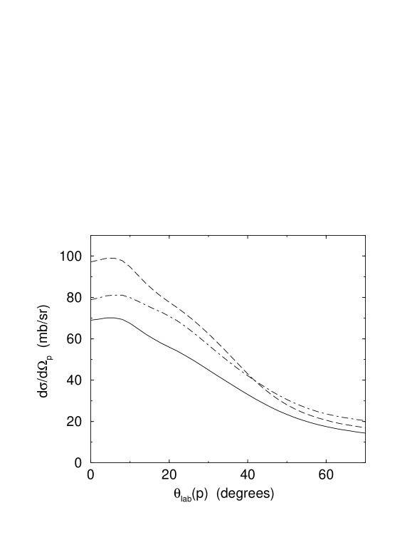
FIG. 8.: Calculated laboratory frame proton cross section angular distributions following the breakup of ⁸B on ⁵⁸Ni at 25.8 MeV, showing the role of the interaction between the proton and the target. The calculations use the EB (solid) and Kim (long dashed) models for the proton-⁷Be interaction and the BG proton-target interaction. The dot-dashed curve uses the EB proton-⁷Be interaction and the VG proton-target interaction.

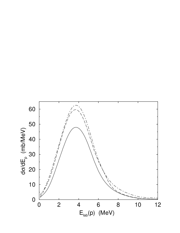
FIG. 9.: Calculated laboratory frame angle integrated proton cross section energy distributions following the breakup of ⁸B on ⁵⁸Ni at 25.8 MeV. The calculations use the EB (solid) and Kim (long dashed) models for the proton-⁷Be interaction and the BG proton-target interaction. The dot-dashed curve uses the EB proton-⁷Be interaction and the VG proton-target interaction.

FIG. 10.: Calculated laboratory frame proton cross section energy distributions following the breakup of ⁸B on ⁵⁸Ni at 25.8 MeV for the ⁷Be fragment laboratory angles indicated. The calculations use the EB proton-⁷Be interaction and the BG proton-target interaction. The arrows indicate 1/8 of the ⁸B energy for elastic scattering at each laboratory angle.

- [1] T. Kobayashi, O. Yamakawa, K. Omata, K. Sugimoto, T. Shimoda, N. Takahashi, and I. Tanihata, Phys. Rev. Lett. 60, 2599 (1988).
- [2] R. Anne et al., Phys. Lett. B250, 19 (1990).
- [3] B. Blank et al., Z. Phys. A340, 41 (1991).
- [4] N. Orr et al., Phys. Rev. Lett. 69, 2050 (1992).
- [5] K. Riisager et al., Nucl. Phys. A540, 565 (1992).
- [6] T. Motobayashi et al., Phys. Rev. Lett. 73, 2680 (1994).
- [7] T. Nakamura et al., Phys. Lett. B331, 296 (1994).
- [8] D. Bazin et al., Phys. Rev. Lett. 74, 3569 (1995).
- [9] W. Schwab et al., Z. Phys. A350, 283 (1995).
- [10] J. von Schwarzenberg, J. J. Kolata, D. Peterson, P. Santi, M. Belbot, and J. D. Hinnefeld, Phys. Rev. C 53, R2598 (1996).
- [11] J. H. Kelley et al., Phys. Rev. Lett. 77, 5020 (1996).
- [12] T. Kikuchi et al., Phys. Lett. B391, 261 (1997).
- [13] D. Bazin et al., Phys. Rev. C 57, 2156 (1998).
- [14] B. Davids et al., Phys. Rev. Lett. 81, 2209 (1998).
- [15] T. Nakamura et al., Phys. Rev. Lett. 83, 1112 (1999).
- [16] N. Iwasa et al., Phys. Rev. Lett. 83, 2910 (1999).
- [17] V. Guimarães et al., Phys. Rev. Lett. 84, 1862 (2000).
- [18] T. Aumann et al., Phys. Rev. C 59, 1252 (1999).
- [19] V. Guimarães et al., Phys. Rev. C 61, 064609 (2000).
- [20] F.M. Nunes and I.J. Thompson, Phys. Rev. C 59, 2652 (1999).
- [21] H. Esbensen and G. Bertsch, Phys. Rev. C 59, 3240 (1999).
- [22] M. Kamimura, M. Yahiro, Y. Iseri, H. Kameyama, Y. Sakuragi, and M. Kawai, Prog. Theor. Phys. Suppl. 89, 1 (1986).
- [23] N. Austern, Y. Iseri, M. Kamimura, M. Kawai, G. Rawitscher, and M. Yahiro, Phys. Rep. 154, 125 (1987).
- [24] J.J. Kolata et al., Phys. Rev. C, submitted.
- [25] I.J. Thompson, Comp. Phys. Rep. 7, 167 (1988); fresco users’ manual, University of Surrey, UK.
- [26] J.S. Al-Khalili and J.A. Tostevin, Few-body models of nuclear reactions, in: “Scattering”, eds. Roy Pike and Pierre Sabatier, Academic Press, Chapter 3.1.4, in the press.
- [27] H. Fuchs, Nucl. Inst. and Meth. 200, 361 (1982).
- [28] F.M. Nunes and I.J. Thompson, Phys. Rev. C 57, R2818 (1998).
- [29] C.H. Dasso, S.M. Lenzi, and A. Vitturi, Nucl. Phys. A639, 635 (1998).
- [30] Z. Moroz, P. Zupranski, R. Bottger, P. Egelhof, K.-H. Mobius, G. Tungate, E. Steffens, W. Dreves, I. Koenig, and D. Fick, Nucl. Phys. A381, 294 (1982).
- [31] H. Esbensen and G. Bertsch, Nucl. Phys. A600, 37 (1996).
- [32] K.H. Kim, M.H. Park, and B.T. Kim, Phys. Rev. C 35, 363 (1987).
- [33] F.D. Becchetti and G.W. Greenlees, Phys. Rev. 182, 1190 (1969).
- [34] C.M. Perey and F.G. Perey, Atomic Data and Nuclear Data Tables 17, 1 (1979).
- [35] F.G. Perey, Phys. Rev. 131, 745 (1963).
- [36] R.A. Vanetsian, A.P. Klyucharev, G.F. Timoshevskii, and E.D. Fedchenko, Sov. Phys. JETP 13, 842 (1961).
- [37] R. Shyam and I.J. Thompson, Phys. Rev. C 59, 2645 (1999).
- [38] J.A. Tostevin, Single-nucleon knockout reactions at fragmentation beam energies, in: Proc. Int. Conf. on nuclear structure (NS2000) (East Lansing, August 15-19 2000), Nucl. Phys. A, in press.