Rearranging Pionless Effective Field Theory

Abstract

We point out a redundancy in the operator structure of the pionless effective field theory, ${\rm EFT}({\pi\hskip-6.00006pt/})$, which dramatically simplifies computations. This redundancy is best exploited by using dibaryon fields as fundamental degrees of freedom. In turn, this suggests a new power counting scheme which sums range corrections to all orders. We explore this method with a few simple observables: the deuteron charge form factor, $np\rightarrow d\gamma$, and Compton scattering from the deuteron. Unlike ${\rm EFT}({\pi\hskip-6.00006pt/})$, the higher dimension operators involving electroweak gauge fields are not renormalized by the s-wave strong interactions, and therefore do not scale with inverse powers of the renormalization scale. Thus, naive dimensional analysis of these operators is sufficient to estimate their contribution to a given process.

I Introduction

An effective field theory (${\rm EFT}({\pi\hskip-6.00006pt/})$) has been constructed that allows for precise calculations of very low-energy nuclear processes. In this energy regime, all multi-nucleon interactions are described by local operators. The relative size of the contribution of an operator to a particular observable can be estimated by the power-counting rules developed in [1, 2, 3, 4, 5, 6, 7]. An array of phenomena have been studied with ${\rm EFT}({\pi\hskip-6.00006pt/})$, such as the radiative capture $np\rightarrow d\gamma$ relevant to Big-Bang nucleosynthesis [9, 10], elastic and inelastic $\nu d$ scattering [11, 12] relevant to the ongoing efforts to measure the solar-neutrino flux and the cross section for $pp\rightarrow de\nu$ [13, 14, 15, 16], the electromagnetic form factors of the deuteron [7, 17], and other processes involving electroweak gauge fields (for a detailed review of this subject see Ref. [18]).

While calculation of such processes to high precision is straightforward, the number of Feynman diagrams involved can become quite large. It was shown that determining the coefficients in the Lagrange density by reproducing the deuteron binding energy, $B$, and the residue of the deuteron pole, $Z_{d}$, at next-to-leading order (NLO) [19], instead of reproducing the scattering length, $a^{({}^{3}\kern-0.98ptS_{1})}$ and effective range, $r^{({}^{3}\kern-0.98ptS_{1})}$ at NLO dramatically improves the convergence of ${\rm EFT}({\pi\hskip-6.00006pt/})$. This is because the effective range in both s-wave channels is somewhat larger than one would naively guess, the expansion parameter in the ${}^{3}\kern-1.4ptS_{1}$ channel being $\gamma r^{({}^{3}\kern-0.98ptS_{1})}\sim 0.4$, where $\gamma^{2}=M_{N}B$ is the deuteron binding momentum.

One of the simplifications we suggest in this work is that $r^{({}^{3}\kern-0.98ptS_{1})}$ should be taken to be of order $1/Q$ in the power counting, a suggestion first made in Ref. [20]. This naturally leads to the use of dibaryon fields, as first discussed in Ref. [21] and profitably exploited in Ref. [22, 23, 24]. In this formulation of ${\rm EFT}({\pi\hskip-6.00006pt/})$, operators are ordered according to powers of the total center-of-mass energy. We will see that this simplification is a consequence of a redundancy in the operator structure of ${\rm EFT}({\pi\hskip-6.00006pt/})$. Moreover, in this modified power counting, dibaryon operators representing higher-dimensional nucleon contact interactions are not renormalized by the s-wave interactions as in standard ${\rm EFT}({\pi\hskip-6.00006pt/})$ [7] and as a consequence are ordered according to naive dimensional analysis. These observations lead to a remarkable simplification in the computation of higher order effects.

II An Operator Redundancy

To begin with, we make the following general observation that simplifies computations in ${\rm EFT}({\pi\hskip-6.00006pt/})$. In higher order calculations, Galilean-invariant operators appear involving a large number of derivatives acting on the incoming and outgoing nucleon fields. By integrating by parts and then using the equations of motion for the nucleon field the number of higher order operators is greatly reduced, and calculations are simplified further by utilizing operators involving time-derivatives and not just spatial derivatives. To show this we consider the interaction Lagrange density that contributes to NN scattering in the ${}^{3}\kern-1.4ptS_{1}$-channel at next-to-next-to-leading order (N²LO) in the EFT expansion,

$${\cal L}^{N^{2}LO} = -C_{4}\left(N^{T}P^{j}(\overleftarrow{\nabla}-\overrightarrow{\nabla})^{2}N\right)^{\dagger}\left(N^{T}P^{j}(\overleftarrow{\nabla}-\overrightarrow{\nabla})^{2}N\right)$$ (2)

$$-{1\over 2}\tilde{C}_{4}\left[\left(N^{T}P^{j}(\overleftarrow{\nabla}-\overrightarrow{\nabla})^{4}N\right)^{\dagger}N^{T}P^{j}N\ +\ {\rm h.c.}\right]\ \ \ ,$$

where the spin-isospin projector for the ${}^{3}\kern-1.4ptS_{1}$ channel is

$$P^{i} \equiv {1\over\sqrt{8}}\sigma_{2}\sigma^{i}\ \tau_{2}\ \ \ ,\ \ \ {\rm Tr}\left[P^{i\dagger}P^{j}\right]\ =\ {1\over 2}\delta^{ij}\ \ \ .$$ (3)

It is straightforward to show that, by using the equations of motion for the nucleon field and integrating by parts where necessary,

$$-\theta\ N^{T}P^{j}(\overleftarrow{\nabla}-\overrightarrow{\nabla})^{2}N = 4M_{N}\ \theta\ \left[i\partial_{0}+{\nabla^{2}\over 4M_{N}}\right]N^{T}P^{j}N\equiv 4M_{N}\ \theta\ {\cal O}_{E}N^{T}P^{j}N\ \ \ ,$$ (4)

where $\theta$ is some operator, and we have not shown terms that are total derivatives. The operator ${\cal O}_{E}$ when acting on the two-nucleon operator simply yields the non-relativistic center-of-mass energy. Therefore, the Lagrange density in eq. (2) becomes

$${\cal L}^{N^{2}LO} = -(4M_{N})^{2}\ \left(C_{4}+\tilde{C}_{4}\right)\left[{\cal O}_{E}N^{T}P^{j}N\right]^{\dagger}{\cal O}_{E}N^{T}P^{j}N\ \ \ ,$$ (5)

and involves only one operator. It is clear how to generalize this result to higher orders in the ${\rm EFT}({\pi\hskip-6.00006pt/})$ expansion, and in fact, there is only one new operator for each higher order in the energy expansion. This is completely consistent with the Effective Range (ER) expansion [25, 26], and with the previous works on ${\rm EFT}({\pi\hskip-6.00006pt/})$ [7] where it was shown that NN scattering constrains only the combination $C_{4}+\tilde{C}_{4}$. An all-orders argument for NN scattering has been given previously [8]. The one place where these operator relations require a little thought is where electroweak currents are inserted. Actually, the above argument holds when derivatives are replaced by covariant derivatives. Previous ${\rm EFT}({\pi\hskip-6.00006pt/})$ calculations have shown that the $C_{4}$ and $\tilde{C}_{4}$ operators contribute differently to electroweak observables. However, it is always a linear combination of these operators and a gauge invariant higher dimension operator that appears, and it is this combination that is fit to data. Thus using the operator structure of eq. (5) will lead to different RG evolution of gauge invariant higher dimension operators compared to that resulting from eq. (2), but physics will be left unchanged. This generalizes the observation made in ref. [27, 28].

III Enter DIBARYONS

If we take seriously the notion that both $a$ and $r$ are of order $Q^{-1}$, then we can describe NN scattering with dibaryon fields in both the ${}^{1}\kern-1.4ptS_{0}$ and ${}^{3}\kern-1.4ptS_{1}$ channels. The Lagrange density describing the dynamics of the dibaryon $t^{j}$ in the ${}^{3}\kern-1.4ptS_{1}$ channel is

$${\cal L}_{t} = N^{\dagger}\left[i\partial_{0}+{\nabla^{2}\over 2M_{N}}\right]N\ -\ t^{\dagger}_{a}\left[i\partial_{0}+{\nabla^{2}\over 4M_{N}}-\Delta\right]t^{a}\ -\ y\left[\ t^{\dagger}_{j}\ N^{T}P^{j}N\ +\ {\rm h.c.}\right]\ \ \ ,$$ (6)

where $y$ is the coupling between nucleons in the ${}^{3}\kern-1.4ptS_{1}$ channel and the ${}^{3}\kern-1.4ptS_{1}$-dibaryon.

FIG. 1.: The dressed dibaryon propagator. The bare dibaryon propagator is dressed by nucleon bubbles to all orders. Each diagram counts as $Q^{-2}$ in the power-counting scheme.

It is easy to show that this Lagrange density alone reproduces the NN scattering amplitude when

$$y^{2} = {8\pi\over M_{N}^{2}r^{({}^{3}\kern-0.98ptS_{1})}}\ \ ,\ \ \Delta\ =\ {2\over M_{N}r^{({}^{3}\kern-0.98ptS_{1})}}\left({1\over a^{({}^{3}\kern-0.98ptS_{1})}}-\mu\right)\ \ \ ,$$ (7)

where $\mu$ is the renormalization scale. As far as power-counting is concerned $y\sim\sqrt{Q}$ and $\Delta\sim Q^{2}$. Therefore, the bare dibaryon propagator counts as $Q^{-2}$, as do arbitrary insertions of nucleon bubbles. Hence the bubbles must be summed to all orders as in Fig. 1. The dibaryon propagator dressed with nucleon bubbles, $D^{({}^{3}\kern-0.98ptS_{1})}(\overline{E})$, as a function of center-of-mass energy $\overline{E}$, is

$$D^{({}^{3}\kern-0.98ptS_{1})}(\overline{E}) = {4\pi\over M_{N}y^{2}}\ {i\over\mu+{4\pi\over M_{N}y^{2}}\Delta-{4\pi\over M_{N}y^{2}}\overline{E}+i\sqrt{M_{N}\overline{E}}}.$$ (8)

The LO scattering amplitude is then

$${\cal A}_{-1} = {{4\pi}\over M_{N}}{1\over-{1\over a^{({}^{3}\kern-0.7ptS_{1})}}+{1\over 2}r^{({}^{3}\kern-0.98ptS_{1})}M_{N}\overline{E}-i\sqrt{M_{N}\overline{E}}}\ \ \ ,$$ (9)

which is simply the effective range expansion, neglecting the shape parameter and higher contributions.

To satisfy oneself that the Lagrange density in eq. (6) reproduces the scattering amplitude that one would obtain by writing down all possible four-nucleon operators, as is done in ${\rm EFT}({\pi\hskip-6.00006pt/})$, it is sufficient to compare the scattering amplitude in the two theories. The exchange of a fully-dressed dibaryon between nucleons is identical to the exact bubble sum, up to terms beyond the effective range, i.e. the shape parameter $r_{1}^{({}^{3}\kern-0.98ptS_{1})}$, and higher. To include the shape parameter, for instance, one includes a term in the Lagrange density,

$${\cal L}^{\rm shape} = -{2M_{N}r_{1}^{({}^{3}\kern-0.98ptS_{1})}\over r^{({}^{3}\kern-0.98ptS_{1})}}\ \left[{\cal O}_{E}t_{j}\right]^{\dagger}\left[{\cal O}_{E}t^{j}\right]\ \ \ .$$ (10)

This operator is suppressed by $Q^{3}$ relative to $\Delta$ and therefore gives rise to a perturbative correction to the LO amplitude via the right diagram in Fig. 2. The $Q^{3}$ suppressed amplitude is thus

$${\cal A}_{2} = -{{4\pi}\over M_{N}}r_{1}^{({}^{3}\kern-0.98ptS_{1})}({M_{N}}\overline{E})^{2}{1\over\left(-{1\over a^{({}^{3}\kern-0.7ptS_{1})}}+{1\over 2}r^{({}^{3}\kern-0.98ptS_{1})}M_{N}\overline{E}-i\sqrt{M_{N}\overline{E}}\right)^{2}}\ \ \ .$$ (11)

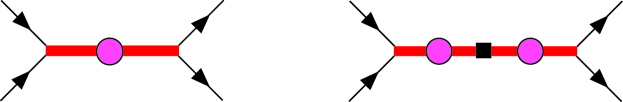
FIG. 2.: Feynman diagrams that contribute to NN scattering. The thick solid lines denote the dibaryon field, while the single lines denote the nucleon field. The black box is an insertion of the shape parameter correction that is suppressed by $Q^{3}$ compared to the LO diagram.

The Lagrange density in eq. (10) demonstrates a general feature of transforming between a theory written in terms of only four-nucleon operators and one written in terms of dibaryons. The “rule” for replacing a nucleon bi-linear with a dibaryon field is, up to numerical factors,

$$N^{T}P^{j}N \rightarrow {1\over\sqrt{M_{N}r^{({}^{3}\kern-0.98ptS_{1})}}}\ t^{j}\ \ \ ,\ \ \ N^{T}\overline{P}^{a}N\rightarrow{1\over\sqrt{M_{N}r^{({}^{1}\kern-0.98ptS_{0})}}}\ s^{a}\ \ \ ,$$ (12)

where $\overline{P}^{a}$ is the projector for the ${}^{1}\kern-1.4ptS_{0}$ channel and $s^{a}$ is the ${}^{1}\kern-1.4ptS_{0}$ dibaryon. This is important to keep in mind as it introduces factors of $\sqrt{Q}$ into the coefficients of operators. The power counting with the effective range scaling as $1/Q$ and a Lagrange density written in terms of dibaryon fields will be denoted by ${\rm dEFT}({\pi\hskip-6.00006pt/})$.

In the most general Lagrange density that describes interactions in or with the ${}^{1}\kern-1.4ptS_{0}$ and ${}^{3}\kern-1.4ptS_{1}$ channels, all higher dimension operators involve couplings to the dibaryon fields, and not to the nucleon bilinear $N^{T}P^{j}N$ in the ${}^{3}\kern-1.4ptS_{1}$ channel or $N^{T}P^{a}N$ in the ${}^{1}\kern-1.4ptS_{0}$ channel. The simplest example of this is perhaps the ${}^{3}\kern-1.4ptS_{1}-{}^{3}\kern-1.4ptD_{1}$ channels. The Lagrange density describing mixing is, up to NLO

$${\cal L}^{(sd)} = -{C_{2}^{(sd)}\over\sqrt{M_{N}r^{({}^{3}\kern-0.98ptS_{1})}}}\ t^{\dagger}_{j}\ N^{T}{\cal O}^{ij}_{\bf(2)}\ P^{i}N\ -\ {C_{4}^{(sd)}\over\sqrt{M_{N}r^{({}^{3}\kern-0.98ptS_{1})}}}\ \left[{\cal O}_{E}t_{j}\right]^{\dagger}\ N^{T}{\cal O}^{ij}_{\bf(2)}\ P^{i}N\ \ +\ \ {\rm h.c.}\ \ ,$$ (13)

with

$${\cal O}^{ij}_{\bf(2)} = -{1\over 4}\left[(\overleftarrow{\nabla}-\overrightarrow{\nabla})^{i}(\overleftarrow{\nabla}-\overrightarrow{\nabla})^{j}-{1\over n-1}\delta^{ij}(\overleftarrow{\nabla}-\overrightarrow{\nabla})^{2}\right]\ \ \ ,$$ (14)

and the ellipses denote operators involving more powers of the center-of-mass energy $\overline{E}$. This leads to a mixing parameter $\overline{\varepsilon}_{1}$ at NLO of

$$\overline{\varepsilon}_{1} = \left[C_{2}^{(sd)}\ +\ C_{4}^{(sd)}\overline{E}\right]{\sqrt{M_{N}}(M_{N}\overline{E})^{3/2}\over 6\sqrt{\pi}}{1\over\sqrt{(-{1\over a^{({}^{3}\kern-0.7ptS_{1})}}+{1\over 2}r^{({}^{3}\kern-0.98ptS_{1})}M_{N}\overline{E})^{2}+M_{N}\overline{E}}}\ \ \ .$$ (15)

Writing this expression in terms of the asymptotic ${}^{3}\kern-1.4ptS_{1}$ to ${}^{3}\kern-1.4ptD_{1}$ ratio $\eta_{sd}$, defined by

$$\eta_{sd} = -\tan\left(\varepsilon_{1}\right)\ \ \ ,\ \ \ \tan\left(2\varepsilon_{1}\right)\ =\ {\tan\left(2\overline{\varepsilon}_{1}\right)\over\sin\left(\overline{\delta}_{0}-\overline{\delta}_{2}\right)}\ \ \ ,$$ (16)

evaluated at the deuteron pole, $|{\bf p}|=i\gamma$,

$$\overline{\varepsilon}_{1} = \eta_{sd}\left({M_{N}\overline{E}\over\gamma^{2}}\right){\sqrt{M_{N}\overline{E}}\over\sqrt{(-{1\over a^{({}^{3}\kern-0.7ptS_{1})}}+{1\over 2}r^{({}^{3}\kern-0.98ptS_{1})}M_{N}\overline{E})^{2}+M_{N}\overline{E}}}\ +\ ...\ \ \ .$$ (17)

The ellipses denote the contribution from the $C_{4}^{(sd)}$ and higher operators.

IV External Probes

For processes involving the deuteron either in the initial, or final states, or both, it is convenient to use sources that couple to the dibaryon fields directly. As we only require the source to have a non-zero overlap with the state of interest, sources coupling to the dibaryon fields are sufficient. In fact, this makes calculations much simpler. To compute S-matrix elements, the residue of the ${}^{3}\kern-1.4ptS_{1}$ dibaryon field is required at the deuteron pole. Writing the dibaryon propagator as

$$G(\overline{E}) = {i{\cal Z}(\overline{E})\over\overline{E}+B}\ =\ {i(Z_{d}+Z_{1}(\overline{E}+B)+...)\over\overline{E}+B}\ \ \ ,$$ (18)

gives

$$Z_{d} = {\gamma r^{({}^{3}\kern-0.98ptS_{1})}\over 1-\gamma r^{({}^{3}\kern-0.98ptS_{1})}}\ \ \ .$$ (19)

In order to demonstrate the simplifications that arise for processes involving electroweak currents, we consider the deuteron charge form factor, $np\rightarrow d\gamma$ and Compton scattering on the deuteron.

A Deuteron Electric Form Factor

The LO diagrams that contribute to the deuteron charge form factor in ${\rm dEFT}({\pi\hskip-6.00006pt/})$ are shown in Fig. 3.

FIG. 3.: The LO Feynman diagrams that contribute to the deuteron charge form factor. The thick solid lines denote the dibaryon field, while the thin lines with arrows denote the nucleon field. The crosses are sources of the dibaryon field. LSZ reduction removes the fully dressed dibaryon propagators from the Green functions.

In addition to diagrams where the photon couples to the nucleon, there are also couplings to the dibaryon field obtained by gauging the Lagrange density in eq. (6). At higher orders there are contributions from higher dimension operators involving more derivatives on the nucleon field, such as the nucleon charge radius operator, and also from higher dimension couplings of the dibaryon, such as the dibaryon charge radius. It is interesting to note that these higher dimension operators are not renormalized by the s-wave strong interactions, as is the case when four-nucleon operators alone are used to describe the s-wave scattering amplitude. Therefore, the size of the contribution of the higher dimension operators can be estimated simply by counting the dimensions of the operator and including the appropriate powers of the high scale $\Lambda$ in its coefficient. The contribution to the charge form factor from the tree-level photon coupling to the dibaryon is, (removing a factor of $ie$ from the amplitude)

$$\Gamma^{(a)} = 1\ \left(\sqrt{Z_{d}}\right)^{2}\ \ \ ,$$ (20)

and from the nucleon loop diagram is

$$\Gamma^{(b)} = -{4\over|{\bf q}|\ r^{({}^{3}\kern-0.98ptS_{1})}}\tan^{-1}\left({|{\bf q}|\over 4\gamma}\right)\left(\sqrt{Z_{d}}\right)^{2}\ \ \ ,$$ (21)

where $|{\bf q}|$ is the magnitude of the photon three-momentum. These contributions combine to give a charge form factor of

$$F_{C}(|{\bf q}|) = {\gamma r^{({}^{3}\kern-0.98ptS_{1})}\over 1-\gamma\ r^{({}^{3}\kern-0.98ptS_{1})}}\left[{4\over|{\bf q}|\ r^{({}^{3}\kern-0.98ptS_{1})}}\tan^{-1}\left({|{\bf q}|\over 4\gamma}\right)\ -\ 1\ \right]\ \ \ .$$ (22)

This reproduces the result of ER theory, as expected. At higher orders in the effective field theory expansion there will be a contribution from the nucleon form factor, starting with the nucleon charge radius[7] at order $Q^{2}$. At order $Q^{3}$ there is a contribution from the dibaryon charge radius operator.

B $np\rightarrow d\gamma$

The radiative capture process $np\rightarrow d\gamma$ at low-energy has been computed with $\sim 1\%$ accuracy with ${\rm EFT}({\pi\hskip-6.00006pt/})$ [9, 10]. The process is dominated by the $E1$ and $M1$ multipoles, for which the matrix element is

$${\cal A} = e\ X_{E1}\ U^{T}_{n}\sigma_{2}\ \sigma\cdot\epsilon_{(d)}^{*}U_{p}\ {\bf p}\cdot\epsilon_{(\gamma)}^{*}\ +\ i\ e\ X_{M1}\ \varepsilon^{abc}\ \epsilon_{(d)}^{*a}\ {\bf k}^{b}\ \epsilon_{(\gamma)}^{*c}\ U^{T}_{n}\sigma_{2}U_{p}\ \ ,$$ (23)

where ${\bf k}$ and $\epsilon_{(\gamma)}$ are the photon momentum and polarization vector, $\epsilon_{(d)}$ is the deuteron polarization vector and $U_{n,p}$ are the neutron and proton spinors; ${\bf p}$ is the momentum of the proton in the center-of-momentum frame. It is convenient to define dimensionless variables $\tilde{X}_{\pi L}$,

$${|{\bf p}|M_{N}\over\gamma^{2}+|{\bf p}|^{2}}X_{E1}\ = i{2\over M_{N}}\sqrt{\pi\over\gamma^{3}}\tilde{X}_{E1}\quad,\quad X_{M1}\ \ =\ i{2\over M_{N}}\sqrt{\pi\over\gamma^{3}}\tilde{X}_{M1}\ \ \ ,$$ (24)

in terms of which the total cross section is

$$\sigma = {4\pi\alpha(\gamma^{2}+|{\bf p}|^{2})^{3}\over M_{N}^{4}\gamma^{3}|{\bf p}|}\left[\ |\tilde{X}_{M1}|^{2}\ +\ |\tilde{X}_{E1}|^{2}\ \right]\ \ \ .$$ (25)

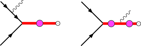
FIG. 4.: The diagrams providing the LO contribution to the $E1$ amplitude, $\tilde{X}_{E1}$. The photon is minimally coupled.

The diagrams shown in Fig. 4 provide the LO contributions to the $E1$ amplitude in ${\rm dEFT}({\pi\hskip-6.00006pt/})$. Up to order $Q^{2}$, the $E1$ amplitude is given by

$$\tilde{X}_{E1} = -{1\over\sqrt{1-\gamma r^{({}^{3}\kern-0.98ptS_{1})}}}\ {|{\bf p}|M_{N}\gamma^{2}\over(|{\bf p}|^{2}+\gamma^{2})^{2}}\ \ \ ,$$ (26)

consistent with ER theory at this order. A higher dimension operator coupling an E1 photon to a ${}^{3}\kern-1.4ptS_{1}$-dibaryon and a p-wave two nucleon final state is suppressed by $Q^{3}$ in the power counting.

The $M1$ amplitude receives contributions from the magnetic moments of the nucleon and from four-nucleon operators coupling to the magnetic field, which are described by the Lagrange density involving dibaryon fields

$${\cal L}^{\bf B} = {e\over 2M_{N}}N^{\dagger}\left(\kappa_{0}+\kappa_{1}\tau^{3}\right)\sigma\cdot{\bf B}\ N\ +\ e\ {L_{1}\over M_{N}\sqrt{r^{({}^{1}\kern-0.98ptS_{0})}\ r^{({}^{3}\kern-0.98ptS_{1})}}}\ t^{j\dagger}s_{3}{\bf B}_{j}\ \ \ +\ \ {\rm h.c.},$$ (27)

where $t_{j}$ is the ${}^{3}\kern-1.4ptS_{1}$ dibaryon and $s_{a}$ is the ${}^{1}\kern-1.4ptS_{0}$ dibaryon. The unknown coefficient $L_{1}$, which contributes at order $Q$ (compared to the $\kappa_{1}$ contributions) must either be predicted from QCD or determined experimentally in order to have model-independent predictive power.

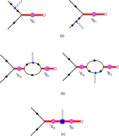
FIG. 5.: Diagrams contributing to the $M1$ amplitude for $np\rightarrow d\gamma$ capture from the ${}^{1}\kern-1.4ptS_{0}$ channel. The thick lines correspond to either ${}^{1}\kern-1.4ptS_{0}$ or ${}^{3}\kern-1.4ptS_{1}$ dibaryons, while the thin lines represent nucleons. The solid circles correspond to an insertion of the single nucleon $\sigma\cdot{\bf B}$ operator. The solid square in diagram (c) denotes the insertion of a four-nucleon-magnetic-photon operator described by a coupling between the ${}^{1}\kern-1.4ptS_{0}$-dibaryon and the ${}^{3}\kern-1.4ptS_{1}$-dibaryon and a magnetic photon.

The diagrams in Fig. 5 (a) and (b) are the LO contributions to the $M1$ amplitude for capture from the ${}^{1}\kern-1.4ptS_{0}$ channel. The diagram in Fig. 5 (c) enters at NLO and represents the contribution from the four-nucleon-one-magnetic-photon operator at this order. It is straightforward to show that the sum of the diagrams in Fig. 5 gives

$$\tilde{X}_{M1} = {1\over\sqrt{1-\gamma r^{({}^{3}\kern-0.98ptS_{1})}}}\ {1\over-{1\over a^{({}^{1}\kern-0.7ptS_{0})}}+{1\over 2}r^{({}^{1}\kern-0.98ptS_{0})}|{\bf p}|^{2}-i|{\bf p}|}$$ (29)

$$\left[\ \kappa_{1}\ {\gamma^{2}\over|{\bf p}|^{2}+\gamma^{2}}\left(\gamma-{1\over a^{({}^{1}\kern-0.98ptS_{0})}}+{1\over 2}r^{({}^{1}\kern-0.98ptS_{0})}|{\bf p}|^{2}\right)\ +\ L_{1}\ {\gamma^{2}\over 2}\ \right]\ \ \ ,$$

which reproduces the results of Ref. [9] when expanded out to lowest order in the effective ranges. In calculating $\tilde{X}_{M1}$ in eq. (29) we have used non-relativistic kinematics, as the relativistic corrections are small as shown in Ref. [10]. In order to reproduce the measured cross section of $\sigma^{\rm expt}=334.2\pm 0.5~{}{\rm mb}$[29] for an incident neutron speed of $|{\bf v}|=2200~{}{\rm m/s}$ in the laboratory frame, $L_{1}$ is required to be $L_{1}\sim-4.0~{}{\rm fm}$ (where we have worked to linear order in $L_{1}$)

The numerical values of the cross section for $np\rightarrow d\gamma$ one obtains from the expressions in eq. (26) and eq. (29) agree very well with the values obtained in Refs. [9, 10], as expected. The uncertainty in these expressions translates into an uncertainty in the capture cross section in the energy regime relevant for nucleosynthesis of $\sim 3\%$. The difference between this work and that of Refs. [9, 10], is the complexity of the computation. In Refs. [9, 10] multiple (unnested) loop diagrams were computed and the renormalization group evolution of $L_{1}(\mu)$ was non-trivial. In the present computation only one-loop diagrams occur, with the majority of the calculation being tree-level. In addition, $L_{1}$ is not renormalized by the s-wave interactions at this order.

C $\gamma d\rightarrow\gamma d$ Compton Scattering

Finally, we examine Compton scattering in ${\rm dEFT}({\pi\hskip-6.00006pt/})$. Working in the zero-recoil limit, and neglecting relativistic effects (both of which are very small) we compute the cross section for the scattering of unpolarized photons from unpolarized deuterons in the low energy regime. This process has been computed in ${\rm EFT}({\pi\hskip-6.00006pt/})$ in Ref. [30]. Writing the amplitude for this process in terms of two form factors, $T_{1}$ and $T_{2}$, we have

$${\cal A} = i{e^{2}\over 2M_{N}}\left[\ T_{1}\ \epsilon\cdot\epsilon^{\prime*}\ +\ T_{2}\ \left(\epsilon\times{\bf k}\right)\cdot\left(\epsilon^{\prime*}\times{\bf k}^{\prime}\right)\right]\ \epsilon_{(d)}\cdot\epsilon_{(d)}^{\prime*}\ \ \ ,$$ (30)

where ${\bf k}$ and $\epsilon$ are the three-momenta and polarization vector of the incident photon, and ${\bf k}^{\prime}$ and $\epsilon^{\prime}$ are the three-momenta and polarization vector of the scattered photon; $\epsilon_{(d)}$ and $\epsilon_{(d)}^{\prime}$ are the polarization vectors of the initial and final state deuteron. As we are neglecting recoil and relativistic effects we will not recover the factor of $M_{d}$ in the coefficient of eq. (30). It was shown in Ref.[7] that $M_{d}$ is recovered order-by-order in perturbation theory in $1/M_{N}$.

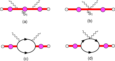
FIG. 6.: Leading-order diagrams contributing to the $T_{1}$ amplitude for $\gamma d\rightarrow\gamma d$ Compton scattering. The thick lines correspond to a ${}^{3}\kern-1.4ptS_{1}$ dibaryon, while the thin lines represent nucleons. The photons are minimally coupled to both the nucleon and the dibaryon. Crossed diagrams are not shown.

The differential cross section resulting from eq. (30) is

$${d\sigma\over d\Omega_{\rm lab}} = {\alpha^{2}\over 8M_{N}^{2}}\left[\ \left(|T_{1}|^{2}+|T_{2}|^{2}\right)\left(1+\cos^{2}\theta\right)\ +\ 4{\rm Re}\left(T_{1}T_{2}^{*}\right)\cos\theta\ \right]\ \ \ .$$ (31)

For the purposes of this discussion we will use Regime II Q-counting [31] where $\gamma\sim\omega\sim Q$ to determine the size of a diagram contributing to the scattering amplitudes. The diagrams shown in Fig. 6 contribute to the electric form factor $T_{1}$ in eq. (31). Figs. 6 (a), (b) and (d) contribute at order $Q^{0}$. Fig. 6 (c) contributes at order $Q^{1/2}$ and higher. It is straightforward to show that

$$T_{1}^{+\omega} = {1\over 1-\gamma r^{({}^{3}\kern-0.98ptS_{1})}}\left[\ {1\over 2}\gamma r^{({}^{3}\kern-0.98ptS_{1})}\ +\ {2\gamma\over 3}{\gamma+2\sqrt{\gamma^{2}+M_{N}\omega-i\epsilon}\over\left(\gamma+\sqrt{\gamma^{2}+M_{N}\omega-i\epsilon}\right)^{2}}\right.$$ (34)

$$\left.\qquad-\ {4\gamma\over\omega\sqrt{2-2\cos\theta}}\tan^{-1}\left({\omega\sqrt{2-2\cos\theta}\over 4\gamma}\right)\ +\ {\omega^{2}\cos\theta\over 6}{\gamma+3\sqrt{\gamma^{2}+M_{N}\omega-i\epsilon}\over\left(\gamma+\sqrt{\gamma^{2}+M_{N}\omega-i\epsilon}\right)^{3}}\right.$$

$$\left.\qquad\ +\ {4M_{N}\pi\left(\alpha_{p}+\alpha_{n}\right)\omega^{2}\over e^{2}}{4\gamma\over\omega\sqrt{2-2\cos\theta}}\tan^{-1}\left({\omega\sqrt{2-2\cos\theta}\over 4\gamma}\right)\ \right]\ \ \ ,$$

where $\omega$ is the incident photon energy. The electric form factor is $T_{1}=T_{1}^{+\omega}+T_{1}^{-\omega}$, with $T_{1}\rightarrow-1$ in the $\omega\rightarrow 0$ limit, as required. We have included the contribution from the nucleon electric polarizabilities, which are defined in the Lagrange density

$${\cal L}_{1} = 2\pi\alpha_{n}\ n^{\dagger}n\ {\bf E}^{2}\ +\ 2\pi\alpha_{p}\ p^{\dagger}p\ {\bf E}^{2}\ +\ 2\pi\beta_{n}\ n^{\dagger}n\ {\bf B}^{2}\ +\ 2\pi\beta_{p}\ p^{\dagger}p\ {\bf B}^{2}\ \ \ ,$$ (35)

and which contribute through the diagrams shown in Fig. 7 at order $Q^{2}$.

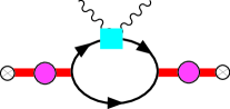
FIG. 7.: Contribution to $T_{1}$ and $T_{2}$ from the electric and magnetic polarizabilities of the nucleon. The solid square denotes an insertion of the nucleon polarizability operators.

The zero-range limit of $T_{1}$ coincides with previous computations [31, 32].

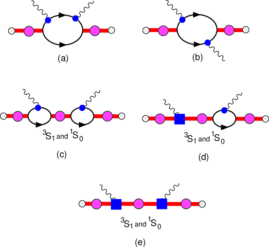
FIG. 8.: Diagrams contributing to the $T_{2}$ amplitude for Compton scattering. The thick lines correspond to either a ${}^{1}\kern-1.4ptS_{0}$ or ${}^{3}\kern-1.4ptS_{1}$ dibaryon, while the thin lines represent nucleons. The photons couple to the nucleons via the $\sigma\cdot{\bf B}$ interaction, represented by the small solid circle. The solid square denotes coupling between the photon and dibaryons due to the higher dimension operators, e.g. the $L_{1}$ operator that contributes to $np\rightarrow d\gamma$. Crossed diagrams are not shown.

The magnetic form factor is dominated by the diagrams shown in Fig. 8, and can be shown to be

$$T_{2}^{+\omega} = {1\over 1-\gamma r^{({}^{3}\kern-0.98ptS_{1})}}\left[\ {4\kappa_{1}^{2}\gamma\over 3M_{N}^{2}\omega^{2}}{\left(\gamma-\sqrt{\gamma^{2}+M_{N}\omega-i\epsilon}\right)\left(\gamma-{1\over a^{({}^{1}\kern-0.98ptS_{0})}}-{1\over 2}r^{({}^{1}\kern-0.98ptS_{0})}\left(\gamma^{2}+M_{N}\omega\right)\right)\over-{1\over a^{({}^{1}\kern-0.7ptS_{0})}}-{1\over 2}r^{({}^{1}\kern-0.98ptS_{0})}\left(\gamma^{2}+M_{N}\omega\right)+\sqrt{\gamma^{2}+M_{N}\omega-i\epsilon}}\right.$$ (41)

$$\left.\quad+\ {4\gamma\kappa_{1}L_{1}\over 3}{1\over\gamma+\sqrt{\gamma^{2}+M_{N}\omega-i\epsilon}}{1\over-{1\over a^{({}^{1}\kern-0.7ptS_{0})}}-{1\over 2}r^{({}^{1}\kern-0.98ptS_{0})}\left(\gamma^{2}+M_{N}\omega\right)+\sqrt{\gamma^{2}+M_{N}\omega-i\epsilon}}\right.$$

$$\left.\quad+\ {\gamma L_{1}^{2}\over 3}{1\over-{1\over a^{({}^{1}\kern-0.7ptS_{0})}}-{1\over 2}r^{({}^{1}\kern-0.98ptS_{0})}\left(\gamma^{2}+M_{N}\omega\right)+\sqrt{\gamma^{2}+M_{N}\omega-i\epsilon}}\right.$$

$$\left.\quad+\ {2\kappa_{0}^{2}\gamma(r^{({}^{1}\kern-0.98ptS_{0})})^{2}\over 3}{1\over\sqrt{\gamma^{2}+M_{N}\omega-i\epsilon}-\gamma-{1\over 2}M_{N}r^{({}^{1}\kern-0.98ptS_{0})}\omega}\right.$$

$$\left.\quad-\ {1\over 6}{\gamma+3\sqrt{\gamma^{2}+M_{N}\omega-i\epsilon}\over\left(\gamma+\sqrt{\gamma^{2}+M_{N}\omega-i\epsilon}\right)^{3}}\right.$$

$$\left.\quad\ +\ {4M_{N}\pi\left(\beta_{p}+\beta_{n}\right)\over e^{2}}{4\gamma\over\omega\sqrt{2-2\cos\theta}}\tan^{-1}\left({\omega\sqrt{2-2\cos\theta}\over 4\gamma}\right)\right]\ \ \ ,$$

where $T_{2}=T_{2}^{+\omega}+T_{2}^{-\omega}$ and where we have included the contribution from the magnetic polarizabilities of the nucleon, $\beta_{p}$ and $\beta_{n}$, entering from diagrams of the form shown in Fig. 7. Figs. 8(a-c) are the leading contributions at order $Q$ and higher, Fig. 8(d) contributes at order $Q^{2}$ and higher while Fig. 8(e) contributes at order $Q^{3}$. The nucleon magnetic polarizabilities enter at order $Q^{2}$.

It is clear from these expressions that they are precisely what one would obtain from ER theory when only the single nucleon operators are retained. However, deviations from ER theory occur due to the presence of four-nucleon local interactions with the electric and magnetic field[31, 33], such as the $L_{1}$ operator and also interactions of the form

$${\cal L} = {2\pi\alpha_{4}\over M_{N}r^{({}^{3}\kern-0.98ptS_{1})}}t_{j}^{\dagger}t^{j}|{\bf E}|^{2}\ +\ {2\pi\beta_{4}\over M_{N}r^{({}^{3}\kern-0.98ptS_{1})}}t_{j}^{\dagger}t^{j}|{\bf B}|^{2}\ +\ ...\ \ ,$$ (42)

that directly couple dibaryons to two-photons, entering at the same order as the $L_{1}^{2}$ contribution in eq. (41). The contributions to Compton scattering from these higher dimension operators, as shown in Fig. 9, are of order $Q^{3}$, and so enter at one order higher than the nucleon polarizabilities themselves. So it appears that the nucleon polarizabilities can be determined from Compton scattering only with precision of order $Q$, due to the presence of higher dimension operators, corresponding to the polarizabilities of the dibaryon itself.

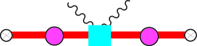
FIG. 9.: Insertion of a higher dimension operator contributing to Compton scattering. The solid square denotes an insertion of the dibaryon electric or magnetic polarizability.

The differential cross section for an incident photon energy of $\omega=49~{}{\rm MeV}$ resulting from the calculated $T_{1}$ and $T_{2}$ is shown in Fig. 10. Even though $\omega=49~{}{\rm MeV}$ is quite possibly above the energy at which the pionless theory makes sense, it is nonetheless useful to see the impact that the nucleon polarizabilities have on the differential cross section. The solid curve in Fig. 10 includes the contribution from the individual nucleon polarizabilities as computed at one-loop order in chiral perturbation theory [34],

$$\alpha_{N} = 10\beta_{N}\ =\ {5g_{A}^{2}e^{2}\over 192\pi^{2}f_{\pi}^{2}m_{\pi}}\ =\ 1.2\times 10^{-3}\ {\rm fm}^{3}\ \ \ \ .$$ (43)

It is clear that high precision measurements of the Compton scattering cross section at low-energies will allow for a reasonable determination of the nucleon isoscalar electric polarizability, and possibly the isoscalar magnetic polarizability. As the contribution from the nucleon polarizabilities scales like $\omega^{2}$, the lower the energy of the incident photon the higher the precision of the measurement that is required to provide a comparable constraint on the polarizabilities.

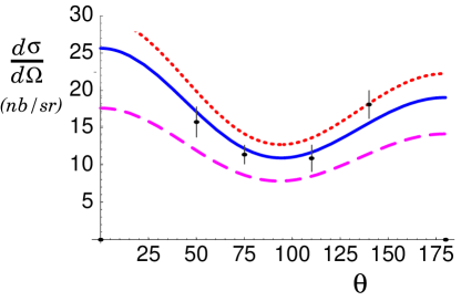
FIG. 10.: Differential cross section for $\gamma d\rightarrow\gamma d$ for an incident photon energy of $\omega=49~{}{\rm MeV}$. The dashed curve is the zero-range limit of the cross section, i.e. $r^{({}^{1}\kern-0.98ptS_{0})}=r^{({}^{3}\kern-0.98ptS_{1})}=0$. The dotted curve corresponds to the full calculation but with the nucleon polarizabilities set equal to zero, i.e. $\alpha_{N}=\beta_{N}=0$. The solid curve is the full calculation including the nucleon polarizabilities being set equal to their value computed at one-loop in chiral perturbation theory [34]. The data is from Ref. [35].

V Conclusion

We have solidified three ideas that allow for much simpler calculations of low-energy nuclear observables using effective field theory. First, we have shown that by using the nucleon equations of motion and judiciously integrating by parts, the number of higher dimension four-nucleon operators is greatly reduced. Second, we have suggested that the large corrections arising from the effective range parameter in both the ${}^{1}\kern-1.4ptS_{0}$ and ${}^{3}\kern-1.4ptS_{1}$ channels can be resummed by taking the range parameter to scale as $1/Q$, just like the scattering length. Third, we have taken the idea of using dibaryon fields seriously and have shown that their use reduces the labor of computing higher order corrections in processes with external gauge fields substantially. Unlike in ${\rm EFT}({\pi\hskip-6.00006pt/})$, in ${\rm dEFT}({\pi\hskip-6.00006pt/})$ two-nucleon higher dimension operators are not renormalized by leading-order four-nucleon operators, and hence one can estimate the contributions of such operators by naive dimensional analysis, in terms of the high scale $\Lambda$. It is important to realize that ${\rm dEFT}({\pi\hskip-6.00006pt/})$ does not invalidate ${\rm EFT}({\pi\hskip-6.00006pt/})$ but rather allows the EFT to accomodate a large effective range.

As the theory written in terms of dibaryon fields behaves very differently under renormalization scale evolution than the theory written in terms of local four-nucleon operators, it is conceivable that this new power counting leads to simplifications in the three-nucleon systems beyond those utilized in Ref. [22, 23, 24]. A step in this direction has already been taken in Ref. [36]. This possibility will be further explored in the near future.

It may be the case that this approach will tame the convergence problems encountered in the pionful theory [37] with KSW power counting [3, 4, 5]. In KSW counting the leading order phase shift in both the ${}^{1}\kern-1.4ptS_{0}$ and ${}^{3}\kern-1.4ptS_{1}$ channels tends to $\pi/2$, at energies below $m_{\pi}/2$ (the scale near which the perturbative theory appears to diverge). However, with the dibaryon describing the leading order amplitude, the phase shift is much smaller in this same energy region, and consequently the contribution from higher orders in the KSW expansion are expected to be suppressed by factors of two or three. This idea is yet to be explored, and it will be interesting to see whether this scheme can be made consistent with a perturbative pion.

We would like to thank David Kaplan for useful discussions. We acknowledge useful and in some cases entertaining correspondence with Paulo Bedaque, Jiunn-Wei Chen, Harald Grießhammer, Hans-Werner Hammer, Gautam Rupak, Roxanne Springer and Ubi van Kolck. This work is supported in part by the U.S. Department of Energy under Grant No. DE-FG03-97ER4014.

REFERENCES

- [1] M. Lutz, contribution to the Workshop on the Standard Model at Low-Energies: Miniproceedings, ed. J. Bijnens and Ulf-G. Meißner, (1996), hep-ph/9606301.
- [2] U. van Kolck, in Mainz 1997, Chiral Dynamics: Theory and Experiment, ed. A. M. Bernstein, D. Drechsel, and T. Walcher, (Springer-Verlag, Berlin, 1998).
- [3] D. B. Kaplan, M. J. Savage, and M. B. Wise, Nucl. Phys. B534, 329 (1998).
- [4] D. B. Kaplan, M. J. Savage, and M. B. Wise, Phys. Lett. B424, 390 (1998).
- [5] D. B. Kaplan, M. J. Savage, and M. B. Wise, Phys. Rev. C59, 617 (1999).
- [6] U. van Kolck, Nucl. Phys. A645, 273 (1999).
- [7] J.-W. Chen, G. Rupak, and M. J. Savage, Nucl. Phys. A653, 386 (1999).
- [8] M. C. Birse, J. A. McGovern and K. G. Richardson, Phys. Lett. B464, 169 (1999); hep-ph/9708435.
- [9] J.-W. Chen and M. J. Savage, Phys. Rev. C60, 065205 (1999).
- [10] G. Rupak, Nucl. Phys. A 678, 405 (2000).
- [11] M. Butler and J.-W. Chen, Nucl. Phys. A675, 575 (2000).
- [12] M. Butler, J.-W. Chen, and X. Kong, (2000), nucl-th/0008032.
- [13] X. Kong and F. Ravndal, Nucl. Phys. A656, 421 (1999).
- [14] X. Kong and F. Ravndal, Nucl. Phys. A665, 137 (2000).
- [15] X. Kong and F. Ravndal, Phys. Lett. B470, 1 (1999).
- [16] X. Kong and F. Ravndal, (2000), nucl-th/0004038.
- [17] J.-W. Chen, G. Rupak, and M. J. Savage, Phys. Lett. B464, 1 (1999).
- [18] S. R. Beane, P. F. Bedaque, W. C. Haxton, D. R. Phillips and M. J. Savage, nucl-th/0008064.
- [19] D. R. Phillips, G. Rupak, and M. J. Savage, Phys. Lett. B473, 209 (2000).
- [20] D. B. Kaplan and J. V. Steele, Phys. Rev. C60, 0604002 (1999).
- [21] D. B. Kaplan, Nucl. Phys. B494, 471 (1997).
- [22] P.F. Bedaque, H.-W. Hammer, and U. van Kolck, Nucl. Phys. A646, 444 (1999).
- [23] P.F. Bedaque and H. W. Grießhammer, Nucl. Phys. A671, 357 (2000).
- [24] F. Gabbiani, P.F. Bedaque and H. W. Grießhammer, Nucl. Phys. A675, 601 (2000).
- [25] H. A. Bethe, Phys. Rev. 76, 38 (1949).
- [26] H. A. Bethe and C. Longmire, Phys. Rev. 77, 647 (1950).
- [27] R. J. Furnstahl and H. -W. Hammer, Nucl. Phys. A 678, 277 (2000).
- [28] R. J. Furnstahl, H. -W. Hammer, N. Tirfessa, nucl-th/0010078.
- [29] A.E. Cox, S.A.R. Wynchank and C.H. Collie, Nucl. Phys. 74, 497 (1965).
- [30] H. W. Grießhammer and G. Rupak, in preparation.
- [31] J.-W. Chen, H. W. Grießhammer, M. J. Savage and R. P. Springer, Nucl. Phys. A 644, 245 (1998).
- [32] M. I. Levchuk and A. I. L’vov, Nucl. Phys. A 674, 449 (2000).
- [33] J.-W. Chen, H. W. Grießhammer, M. J. Savage and R. P. Springer, Nucl. Phys. A 644, 221 (1998).
- [34] V. Bernard, N. Kaiser and Ulf-G. Meißner, Phys. Rev. Lett. 67, 1515 (1991); Nucl. Phys. B 373, 364 (1992); Phys. Lett. B 319, 269 (1993).
- [35] M. A. Lucas, Ph. D. thesis, University of Illinois at Urbana-Champaign (1994).
- [36] I. V. Simenog and D. V. Shapoval, Sov. J. Nucl. Phys. 47,620 (1988).
- [37] S. Fleming, T. Mehen and I. W. Stewart, Nucl. Phys. A 677, 313 (2000).