The $\beta\beta 2\nu$-decay in ${}^{48}Ca$

Abstract

A schematic study of the $\beta\beta 2\nu$-decay of ${}^{48}Ca$ is made in a shell-model approach. The emphasis is especially put on the role of the spin-orbit potential in relation with the contribution of other terms in the strong interaction. This is discussed with a particular attention to the behavior of these ones under the $SU(4)$ symmetry. Different methods in calculating the transition amplitude are also looked at with the aim to determine their reliability and, eventually, why they don’t work. Further aspects relative to the failure of the Operator Expansion Method to reproduce the results of more elaborate calculations are examined.

I INTRODUCTION

The importance of the double beta decay process is well recognized. First, the neutrinoless mode, yet unobserved, is of fundamental interest, as it will be a signal for neutrino mass and lepton number non-conservation. Second, the double beta decay with two-neutrino emission ($\beta\beta 2\nu),$ allowed in the standard model, is a very rare process which has not been experimentally observed until 1987, in the decay of ${}^{82}Se$ studied by Elliot et al. [1]. Subsequent results in other nuclei were obtained by other groups (see [2] for a recent review of the experimental situation). Recently Balysh et al. [3] have measured the double beta decay half-life of ${}^{48}Ca.$ This nucleus is the lightest one for which such a measurement is feasible.

On the theoretical side (see [4, 5] for a recent review) the $\beta\beta 2\nu$-decay which, at the beginning, was a well defined process in the standard model, has revealed as a real challenge for nuclear model practitioners. There are two reasons to this situation. On the one hand, the decay mode is highly suppressed and sensitively depends on poorly determined parts of the nuclear interaction. On the other, it is a second order process, which implies a summation on intermediate, and not always well determined, states. Thus, even if it is not a process involving new fundamental physics, the $\beta\beta 2\nu$-decay is related to a new type of nuclear matrix element. This one incorporates information on the wave functions that is not given by other standard observables.

The difficulties in the calculation of the $\beta\beta 2\nu$-decay have been expressed in several different but related ways in the literature:

• In QRPA calculations, it has been related to the extreme sensitivity of the transition matrix element to the so-called $g_{pp}$ parameter, which governs the $pn$-excitations [6, 7, 8].

• In the $SU(4)$ language, it has been connected to poor determination of the nuclear force in the $L=0,\,S=1,\,T=0$ ($J=1^{+}\,T=0)$ channel [9, 8]. At the same time, it was also observed in this scheme that strong truncation of the model basis can produce undesirable contributions to the transition matrix element.

• It has been also connected to the bad description of the $\beta^{+}$ decays, which processes have been used to fit the unknown parts of the nuclear force [7].

In order to avoid some of the previous uncertainties, an alternative approach has been proposed, the Operator Expansion Method (OEM) [10, 11, 12].

In the present paper, we will focus our attention on the role of different parts of the nuclear force in the $\beta\beta 2\nu$-decay as well as on different methods used in the literature to describe this process. For that purpose, the simplest nuclear transition to be studied is the $\beta\beta 2\nu$-decay in ${}^{48}Ca$, that offers a double advantage. There exist both a sensitive experimental value $\left(T_{1/2}^{2\nu}=\left(4.3{+2.4\atopwithdelims. .-1.1}\left[Stat\right]\pm 1.4\left[Syst\right]\right)\times 10^{19}\mathop{\rm y}\cite[cite]{[\@@bibref{Number}{Balysh}{}{}]}\right)$ and an elaborate shell model calculation [13], which is the natural calculation scheme for this nucleus. While doing these studies, we will have in mind a long standing problem. Different calculations were approximately leading to the same decay rate whereas the intrinsic sign of the transition matrix element was not the same [14], requiring some clarification. With this respect, we will in particular show how higher order effects in the $SU(4)$ symmetry breaking interaction modify previous estimates. On the other hand, a critical study of the OEM approach has been done in [15]. Based on an analysis of the $SU(4)$ symmetry breaking effects, other features of the OEM have been revealed, which deserve discussion. Our work is therefore concerned more with the role of various approximations than with a realistic calculation of the process. We will use an analytical force to achieve this objective. This allows us to easily compare various methods of calculation and to switch on and off the different parts of the interaction.

The plan of the paper is as follows. We remind in the second section expressions for the standard transition operator and that one obtained in the OEM approach. In section 3, we introduce in the OEM expression the Coulomb splitting effect and make a comparison of the corresponding result with the transition operator derived independently at the first order in the $SU(4)$ symmetry breaking interaction. The effective NN interaction that we will use for our study is specified in section 4. The fifth section is devoted to a presentation of our results together with a discussion.

II THE $\beta\beta 2\nu$-DECAY: DESCRIPTION OF THE TRANSITION OPERATOR

The $\beta\beta 2\nu$-decay is allowed in the Standard Model. In this process, two neutrons decay to two protons with the emission of two electrons and two neutrinos. The Lagrangian responsible for that process is the standard Fermi one. Under the usual assumptions (the impulse approximation is assumed, the lepton energies are replaced by their average values and non-conservation of isospin is discarded), we obtain that the life time is expressed by

$$\left[T_{1/2}^{\beta\beta 2\nu}\right]^{-1}=G_{2\nu}\left|M_{{\cal GT}}\right|^{2},$$ (1)

where $G_{2\nu},$ which can be found in [4, 16], contains all the leptonic part and the integral on the phase space. The nuclear information is included in the nuclear matrix element

$$M_{{\cal GT}}=\frac{i}{2}\int_{0}^{\infty}dt\,e^{i\Delta t}<0_{f}^{+}|\left[e^{iHt}\vec{A}e^{-iHt},\vec{A}\right]|0_{i}^{+}>,$$ (2)

with $\vec{A}=\sum\vec{\sigma}_{i}\tau_{i}^{+},$ the Gamow-Teller operator, and $\Delta=\frac{1}{2}\left(E_{i}-E_{f}\right)$.

Methods for evaluating the $\beta\beta 2\nu$-decays differ in the approximations made in order to calculate (2). What we will call the standard method consists to insert a complete set of intermediate states in the commutator (2). This allows one to perform the time integral and we obtain

$$M_{{\cal GT}}^{St}=\sum_{n}\frac{<0_{f}^{+}|\vec{A}|1_{n}^{+}><1_{n}^{+}|\vec{A}|0_{i}^{+}>}{E_{n}-\frac{1}{2}\left(E_{i}+E_{f}\right)}.$$ (3)

Theoretically this method is exact, but in practical calculations some limitation occurs. Estimating the matrix element given by Eq. (3) implies to consider all the intermediate states contributing to the sum. Thus, the method could not be the most interesting one if the intermediate states or their energies cannot be well determined and if cancellations between different contributions are present. As we will explain later, the approximated $SU\left(4\right)$ symmetry of the nuclear forces tells us that such cancellations must be present in (3), leading to uncertainties in employing this method of calculation.

On the other hand, in general, nuclei which undergo double beta decay are open shell nuclei and the usual formalism for describing them is the QRPA. In that case, there are new difficulties in the evaluation of the $M_{{\cal GT}}^{St}$ amplitude due to the fact that the QRPA is near the collapse for the physical values of the so-called $g_{pp}$ parameter. Improvements of the QRPA, like full-QRPA, renormalized QRPA or full-RQRPA, can solve these problems but other ones arrive, like the violation of the Ikeda sum rule (see discussion in ref. [4, 5], and see also [17]).

As mentioned in the introduction, the above difficulties have been a source of concern. An alternative approach to calculate directly the exponentials appearing in (2), the operator expansion method (OEM) [10, 11, 12], has thus been proposed some years ago. This is impossible in a general manner and the main assumption made by the authors is to only retain two-body operators, which supposes that only the two nucleons involved in the transition are of special interest in the calculation. This is like a spectator approximation in the sense that all the nucleons not involved in the $\beta\beta$ transition don’t contribute to the process. On the other hand, the interaction between the two active nucleons is included to all orders, neglecting some parts as we will explain later. A diagrammatic view of this approach is shown in Fig. 5a.

In the simplest approximation, the kinetic energy term, the spin-orbit and the tensor potentials are neglected in the Hamiltonian $H$ appearing in (2). Under these assumptions, only the central part of the potential contributes. Starting from its expression written as follows

$$H\approx V_{c}=\sum_{i>j}\left[v_{o}\left(r\right)+v_{\tau}\left(r\right)\vec{\tau}_{i}.\vec{\tau}_{j}+v_{\sigma}\left(r\right)\vec{\sigma}_{i}.\vec{\sigma}_{j}+v_{\sigma\tau}\left(r\right)\vec{\tau}_{i}.\vec{\tau}_{j}\,\vec{\sigma}_{i}.\vec{\sigma}_{j}\right]\,\,,$$ (4)

the $\beta\beta 2\nu$-transition amplitude in the OEM approach, first derived by Šimkovic et al. [10] and Ching et al. [11], can be expressed as

$$M_{{\cal GT}}^{OEM}=<0_{f}^{+}|\sum_{i>j}{\cal M}_{i,j}\tau_{i}^{+}\tau_{j}^{+}|0_{i}^{+}>,$$ (5)

with

$${\cal M}_{ij} = \frac{24\left[v_{\sigma}\left(r\right)-v_{\tau}\left(r\right)\right]}{\Delta^{2}-16\left[v_{\sigma}\left(r\right)-v_{\tau}\left(r\right)\right]^{2}}\Omega_{0}\left(ij\right)$$ (7)

$$+\frac{8\left[2v_{\sigma\tau}\left(r\right)-v_{\sigma}\left(r\right)-v_{\tau}\left(r\right)\right]}{\Delta^{2}-16\left[2v_{\sigma\tau}\left(r\right)-v_{\sigma}\left(r\right)-v_{\tau}\left(r\right)\right]^{2}}\Omega_{1}\left(ij\right),$$

where $\Omega_{0,1}$ represents the projector operator on spin 0 and 1 subspaces.

The Gamow-Teller operator is a $SU(4)$ generator. Then, from equation (2), we observe that $M_{{\cal GT}}$ will be zero if the Hamiltonian were $SU(4)$ invariant (we discard transitions between members of the same $SU\left(4\right)$ multiplets). This result is not obvious from (3) where, in the general case, each intermediate state could give a non-zero contribution, the zero being obtained after summation over all intermediate states. Usual nuclear potentials are not so far from the $SU(4)$ symmetry, then we must expect cancellations in the summation present in (3). From this point of view, expression (7) is more transparent, because the condition over the central force to be $SU(4)$ symmetric is just $v_{\sigma}\left(r\right)=v_{\tau}\left(r\right)=v_{\sigma\tau}\left(r\right)$. Notice that in a particular case, actually close to most realistic transitions, the vanishing of the matrix element would result from the fact that the operator $\vec{A}$ in Eq. (3) acting on the final state gives zero.

III OEM AND SU(4) APPROXIMATION

We can improve the OEM model, Eq. (7), by incorporating the contribution of the Coulomb interaction and then make a comparison of the expression so obtained with that one derived in the first order $SU(4)$ symmetry breaking approximation.

The Coulomb interaction is an important ingredient of the spectroscopy of medium-heavy nuclei involving different charges as it provides a few MeV shifts, which compare to the energy splittings produced by the strong interaction itself. For our purpose, we added to this interaction, $H_{s}$, a constant term proportional to the third component of the total isospin of the nucleus

$$H=H_{s}+\Delta_{c}T_{3}.$$ (8)

The above Coulomb force can be easily included in the operator appearing in (5). Using that $\left[T_{3},\vec{A}\right]=\vec{A}$, we obtain the modification of (7) into

$${\cal M}_{ij} =\frac{24\left[v_{\sigma}\left(r\right)-v_{\tau}\left(r\right)\right]}{\left(\Delta+\Delta_{c}\right)^{2}-16\left[v_{\sigma}\left(r\right)-v_{\tau}\left(r\right)\right]^{2}}\Omega_{0}\left(ij\right)$$ (9)

$$+\frac{8\left[2v_{\sigma\tau}\left(r\right)-v_{\sigma}\left(r\right)-v_{\tau}\left(r\right)\right]}{\left(\Delta+\Delta_{c}\right)^{2}-16\left[2v_{\sigma\tau}\left(r\right)-v_{\sigma}\left(r\right)-v_{\tau}\left(r\right)\right]^{2}}\Omega_{1}\left(ij\right).$$ (10)

From the definition of $\Delta$ and (7), we have the relation, $\Delta+\Delta_{c}=\frac{1}{2}\left(E_{i}^{s}-E_{f}^{s}\right),$ where $E_{i}^{s}$ is the strong interaction contribution to the energy of the state.

As we said before, the nuclear forces are not far from the $SU(4)$ symmetry and, if that symmetry were exact, the double beta transition amplitude will be zero when it connects states belonging to different $SU(4)$ multiplets. In order to look at the consistency of our results, it can be useful to study the first order correction of our expressions in the $SU(4)$ breaking parts of the force. Let us write for that

$$H=H_{0}+H_{1},$$ (11)

where $H_{0}$ $(H_{1})$ represents the $SU(4)$ symmetric (breaking) part of the force. The hamiltonian $H_{0}$ is a purely central force and has two terms in the spin-isospin space, one proportional to $1$ and the other proportional to the Casimir of the $SU(4)$ group, $\left(\vec{\tau}_{i}.\vec{\tau}_{j}+\vec{\sigma}_{i}.\vec{\sigma}_{j}+\vec{\tau}_{i}.\vec{\tau}_{j}\,\vec{\sigma}_{i}.\vec{\sigma}_{j}\right)$

$$H_{0}=\sum_{i>j}\left[v_{o}\left(r\right)+\frac{1}{5}\left(v_{\tau}\left(r\right)+v_{\sigma}\left(r\right)+3v_{\sigma\tau}\left(r\right)\right)\left(\vec{\tau}_{i}.\vec{\tau}_{j}+\vec{\sigma}_{i}.\vec{\sigma}_{j}+\vec{\tau}_{i}.\vec{\tau}_{j}\,\vec{\sigma}_{i}.\vec{\sigma}_{j}\right)\right].$$ (12)

The Hamiltonian, $H_{1}$, which is able to give a double beta transition at the first order in the $SU(4)$ symmetry, involves two other combinations of the components appearing in the central force, Eq. (4),

$$H_{1} =\sum_{i>j}\left[\frac{1}{2}\left(v_{\tau}\left(r\right)-v_{\sigma}\left(r\right)\right)\left(\vec{\tau}_{i}.\vec{\tau}_{j}-\vec{\sigma}_{i}.\vec{\sigma}_{j}\right)\right.$$ (13)

$$+\left.\frac{3}{10}\left(v_{\tau}\left(r\right)+v_{\sigma}\left(r\right)-2v_{\sigma\tau}\left(r\right)\right)\left(\vec{\tau}_{i}.\vec{\tau}_{j}+\vec{\sigma}_{i}.\vec{\sigma}_{j}-\frac{2}{3}\vec{\tau}_{i}.\vec{\tau}_{j}\,\vec{\sigma}_{i}.\vec{\sigma}_{j}\right)\right].$$ (14)

Starting with (2), we observe that there are two different situations. First, let us consider a nucleus with only two active nucleons. In that case it is obvious that $\left[H_{0},H_{1}\right]=0,$ and the exponential of the Hamiltonian present in (2) can be splitted in two exponentials relative to $H_{0}$ and $H_{1}$ respectively. The first one, related to $H_{0},$ commutes with all the operators and can be ruled out. The second one, related to $H_{1},$ can be expanded to the first order in $H_{1}$ and we obtain

$$M_{{\cal GT}}^{(2neutrons)}=\frac{1}{2\left(\Delta+\Delta_{c}\right)^{2}}<0_{f}^{+}|\left[\left[H_{1},\vec{A}\right],\vec{A}\right]|0_{i}^{+}>.$$ (15)

Calculating explicitly these commutators, we get

$\displaystyle M_{{\cal GT}}^{(2neutrons)}=\frac{1}{\left(\Delta+\Delta_{c}\right)^{2}}<0_{f}^{+}|\sum_{i>j}\left\{24\left[v_{\sigma}\left(r\right)-v_{\tau}\left(r\right)\right]\Omega_{0}\left(ij\right)\right.$

$$+\left.8\left[2v_{\sigma\tau}\left(r\right)-v_{\sigma}\left(r\right)-v_{\tau}\left(r\right)\right]\Omega_{1}\left(ij\right)\right\}\tau_{i}^{+}\tau_{j}^{+}|0_{i}^{+}>.$$ (16)

This result agrees with the Coulomb corrected OEM expression, Eq. (10), when this one is expanded up to the first order in the $SU(4)$ symmetry breaking.

Surprisingly, a different result is obtained when we consider a nucleus with more than two valence nucleons. In view of its importance for a comparison with the above OEM result, Eq. (10), we give here some detail on its derivation.

Beyond the two valence nucleon case, $\left[H_{0},H_{1}\right]$ doesn’t vanish and from (2) it can be shown that, up to first order in $H_{1}$,

$$M_{{\cal GT}}^{SU(4)}=\frac{i}{2}\int_{0}^{\infty}dt\,e^{i\left(\Delta+\Delta_{c}\right)t}\sum_{n=1}^{\infty}\frac{\left(it\right)^{n}}{n!}<0_{f}^{+}|\mathrel{\mathop{\underbrace{[H_{0,}...[H_{0},}}\limits_{n-1}}[[H_{1},\vec{A}],\vec{A}]]...]|0_{i}^{+}>.$$ (17)

In order to perform the sum present in Eq. (17), let us define an operator ${\cal B=}\left[\left[H_{1},\vec{A}\right],\vec{A}\right]$ and introduce an operator ${\cal C}$ solution of the equation ${\cal B}=\left[H_{0},{\cal C}\right].$ In terms of the ${\cal C}$ operator, (17) can be rewritten as

$$M_{{\cal GT}}^{SU(4)} = \frac{i}{2}\int_{0}^{\infty}dt\,e^{i\left(\Delta+\Delta_{c}\right)t}\sum_{n=1}^{\infty}\frac{\left(it\right)^{n}}{n!}<0_{f}^{+}|\mathrel{\mathop{\underbrace{[H_{0,}...[H_{0},}}\limits_{n}}{\cal C}]...]|0_{i}^{+}>$$ (18)

$$= \frac{i}{2}\int_{0}^{\infty}dt\,e^{i\left(\Delta+\Delta_{c}\right)t}<0_{f}^{+}|\left[e^{iH_{0}t}{\cal C}e^{-iH_{0}t}{\cal-C}\right]|0_{i}^{+}>$$ (19)

$$= \frac{1}{\Delta+\Delta_{c}}<0_{f}^{+}|{\cal C}|0_{i}^{+}>.$$ (20)

The solution of the equation ${\cal B}=\left[H_{0},{\cal C}\right]$ is

$${\cal C}=-i\lim_{\varepsilon\rightarrow 0}\int_{0}^{\infty}dq\,e^{iH_{0}q}{\cal B\,}e^{-iH_{0}q}\,e^{-\varepsilon q}.$$ (21)

Performing this last integration and using the explicit expression of ${\cal B}$, we obtain:

$$M_{{\cal GT}}^{SU(4)}=-\frac{1}{2\left(\Delta+\Delta_{c}\right)^{2}}<0_{f}^{+}|\left[\left[H_{1},\vec{A}\right],\vec{A}\right]|0_{i}^{+}>.$$ (22)

This equation can also be obtained from (3). To do that, we must realize that up to first order in the $H_{1}$ Hamiltonian, the double beta decay implies a transition between different $SU(4)$ multiplet states. In the case of interest here, it involves the state $\left|\left[4,4\right]T=4,S=0\right\rangle$ associated with the ${}^{48}Ca$ ground state and the state $\left|\left[2,2\right]T=2,S=0\right\rangle$ related to the ${}^{48}Ti$ [9]. Then, there is only one intermediate state contributing to the amplitude, which is the Gamow-Teller resonance of the initial state (with an energy $E_{n}=E_{i}+\Delta_{c})$:

$$M_{{\cal GT}}^{SU(4)}=\sum_{n}\frac{<0_{f}^{+}|\vec{A}|1_{n}^{+}><1_{n}^{+}|\vec{A}|0_{i}^{+}>}{\left(E_{i}+\Delta_{c}\right)-\frac{1}{2}\left(E_{i}+E_{f}\right)}=\frac{1}{\left(\Delta+\Delta_{c}\right)}<0_{f}^{+}|\vec{A}.\vec{A}|0_{i}^{+}>,$$ (23)

and $H_{1}$ appears in the mixing in the final nucleus between the two $SU(4)$ representations

$$|0_{f}^{+}>=|0_{f}^{+}>_{0}+\sum_{r}\frac{1}{\left(E_{f}-E_{r}\right)}|0_{r}^{+}>_{0}\,{}_{0}<0_{r}^{+}|H_{1}|0_{f}^{+}>_{0},$$ (24)

where $|0_{f}^{+}>_{0}$ is the pure $SU\left(4\right)$ final state. When we introduce (24) in (23), only states $|0_{r}^{+}>_{0}$ belonging to the same $SU(4)$ supermultiplet as $|0_{i}^{+}>(=|0_{i}^{+}>_{0})$ can give non-zero contribution and the energies of these states are $E_{r}=E_{i}+2\Delta_{c}.$ Then we obtain

$$M_{{\cal GT}}^{SU(4)} =\frac{1}{\left(\Delta+\Delta_{c}\right)}\sum_{r}\frac{1}{\left(E_{f}-E_{r}\right)}\,\,\,_{0}<0_{f}^{+}|H_{1}|0_{r}^{+}>_{0}\,{}_{0}<0_{r}^{+}|\vec{A}.\vec{A}|0_{i}^{+}>_{0}$$ (25)

$$=-\frac{1}{2\,\left(\Delta+\Delta_{c}\right)^{2}}\,\,_{0}<0_{f}^{+}|H_{1}\vec{A}.\vec{A}|0_{i}^{+}>_{0}.$$ (26)

This result is in agreement with Eq. (22) because the other terms present in the double commutator, $<0_{f}^{+}|\left[\left[H_{1},\vec{A}\right],\vec{A}\right]|0_{i}^{+}>$, vanish in the $SU(4)$ limit. The main point here is that this expression has a sign opposite to (15). This is due to the presence of many nucleons operators in the former expression, as we represent in Fig. 5b, while the latter one only contains two-body operators with the consequence to provide the wrong sign in the first order $SU(4)$ symmetry breaking limit. In particular, contributions due to pure Pauli antisymmetrization, as those depicted in Fig. 5c, are not accounted for in the OEM.

More important, in the simplest case where the operator $H_{0}$ in Eq. (17) can be approximated by the sum of the single particle energies, the different commutators appearing in this expression can be calculated. Their contributions, which form a non-convergent geometrical series, are given, up to a factor, by the sum

$$\frac{1}{2}(1+2+4+8+...)(...),$$ (27)

where the first term in the parentheses is that one retained by the OEM. To get these contributions, we used the relation, $E_{i}^{s}-E_{f}^{s}=2\left(\Delta+\Delta_{c}\right)$. Formally, the above sum can be performed with the result

$$\frac{1}{2}\,\frac{1}{1-2}(...)=-\frac{1}{2}(...).$$ (28)

This is the result obtained from a direct calculation, Eq. (22). It specifies in two ways the failure of the OEM demonstrated on a quantitative basis by Engel et al. [15]. i) Among the contributions that are accounted for by the expression, Eq. (17), it indicates which one is retained by the OEM. ii) The energy difference, $E_{i}^{s}-E_{f}^{s}$, implies the single particle energies of nucleons in the initial and final states. These ones involving the core particles, it makes it clear that the various commutators appearing in Eq. (17) involve three and more body operators.

IV THE EFFECTIVE NN POTENTIAL

As mentioned in the introduction, we are motivated in this paper by two different points. First, we want to study the contributions of the different pieces of the nuclear force to the $\beta\beta 2\nu$-decay. Second, we want to compare the two calculation methods presented in the previous section. We will focus on the double beta decay of ${}^{48}Ca$ because it is a nucleus which can be theoretically described in the nuclear shell model and we can do reliable calculations with both methods. To accomplish our objective, we use an analytical force which, therefore, could not be the best one but, as we will observe later on, the results are good enough to make it credible. In this way, we can easily connect and disconnect the different pieces of the force and calculate the matrix elements of the operators present in (7). We have performed our calculations using the OXBASH code ([18]).

The shell model space is the full fp shell with the single particle energies $\epsilon_{f_{7/2}}=0,$ $\epsilon_{p_{3/2}}=2.1MeV,$ $\epsilon_{p_{1/2}}=3.9MeV$ and $\epsilon_{f_{5/2}}=6.5MeV$. We have used for our calculations the Bertsch-Hamamoto force [19]. This force has a central part which in momentum space is given by:

$$V_{c}\left(q\right) =\left(\frac{f}{m_{\pi}}\right)^{2}\left[\frac{1}{3}\vec{\sigma}_{1}.\vec{\sigma}_{2}\,\vec{\tau}_{1}.\vec{\tau}_{2}\frac{m_{\pi}^{2}}{q^{2}+m_{\pi}^{2}}\right.+$$ (29)

$$\left(a_{a}\Pi^{S=0}\Pi^{T=1}+b_{a}\Pi^{S=1}\Pi^{T=0}\right)\frac{m_{a}^{2}}{q^{2}+m_{a}^{2}}+$$ (30)

$$\left(a_{b}\Pi^{S=0}\Pi^{T=1}+b_{b}\Pi^{S=1}\Pi^{T=0}\right)\left.\frac{m_{b}^{2}}{q^{2}+m_{b}^{2}}\right],$$ (31)

with $f=0.97,$ $m_{\pi}$ the pion mass, $m_{a}=2.5\mathop{\rm fm}^{-1},\,m_{b}=4\mathop{\rm fm}^{-1},$ and a tensor part

$$V_{T}\left(q\right) =-\left(\frac{f}{m_{\pi}}\right)^{2}\frac{1}{3}\left(3\vec{\sigma}_{1}.\vec{q}\,\vec{\sigma}_{2}.\vec{q}-\vec{\sigma}_{1}.\vec{\sigma}_{2}q^{2}\right)\hskip 56.9055pt$$ (32)

$$\times\left[\vec{\tau}_{1}.\vec{\tau}_{2}\left(\frac{1}{q^{2}+m_{\pi}^{2}}-\frac{t_{1}}{q^{2}+m_{a}^{2}}\right)-\frac{t_{0}}{q^{2}+m_{a}^{2}}\right]\,.$$ (33)

Bertsch and Hamamoto (B.H.) fitted the parameters of the force in order to reproduce Reid soft-core G matrix elements and used this force to estimate the Gamow-Teller strength at high excitation in ${}^{90}Zr$. The values for these parameters are given in Table I. The main features of this force are: (i) it contains the one-pion exchange, which governs the long range part of the force, both in the central and the tensor terms; (ii) the other terms of the central force are pure $S$ wave interaction; (iii) the attraction in the $S=1,T=0$ channel is bigger than the one in the $S=0,T=1$ channel (thus the pairing in the $T=0$ channel will be greater than the usual pairing in the $T=1$ channel); (iv) the B-H tensor force was fitted to be used only for $L$ even waves (the $T=0$ channel) and in this order only one of $t_{0,1}$ parameters is necessary. The authors of ref. [19] chose $t_{0}=0$ while the tensor interaction in the $T=1$ channel was completely discarded. We have checked that this tensor force, as an effective one, is consistent with the deuteron D-wave. In order to have a simultaneous description of the three nuclei involved in the transition, ${}^{48}Ca$, ${}^{48}Sc$ and ${}^{48}Ti$, we also fitted the average Coulomb displacement in Eq. (8), $\Delta_{c}$, using the relative position of the ground state of ${}^{48}Ca$ to that of ${}^{48}Ti$.

We nevertheless observe that the B-H force evidences some undesirable features when it is applied to the study of the nucleus spectroscopy. For instance, in the region of ${}^{48}Ca$ of interest here: (i) it gives a state density at low energy larger than obtained with other standard potentials like modified versions of the Kuo-Brown G-matrix interaction [20] or [21]; (ii) the splitting between the first $J=0^{+},\,T=1$ state and the first $J=1^{+},\,T=0$ state of ${}^{42}Sc$ has the wrong sign; (iii) if we extend the tensor force as it is in the original B-H force to the $T=1$ channel, it produces quite important matrix elements. What happens is that this force must be used with some short range correlations which will decrease its effective intensity. We will not introduce short range correlations and for this reason and from the fact that a so simple force cannot have unchangeable parameters in a large range of nuclei, we slightly modified the original B-H parameters. (i) we fitted $a_{a}$ and $b_{a}$, reproducing the relative position of the ground states of ${}^{48}Ca$, ${}^{48}Ti$ and the first $J=1^{+}$ state of ${}^{48}Sc.$ This change has reduced the state density in ${}^{48}Sc$ and has also corrected the splitting between the two first $0^{+}$ states of ${}^{42}Ca$ as well as the splitting between the first $0^{+}$ and the first $1^{+}$ states of ${}^{42}Sc$ (these states are important to determine the two-body effective interaction). (ii) we changed $t_{0}$ and $t_{1}$ in such a way that the tensor matrix elements between two particles in the fp shell coupled to $T=1$ has been strongly reduced but without change in the matrix elements of particles coupled to $T=0.$ These parameters are also given in Table I as modified B-H. Due to their limited number, our force is not the most realistic one. Results presented here cannot therefore compete with other ones which rely on a better force. As it can be seen from the results we obtain, they are realistic enough however so that our schematic study makes sense and can provide sensitive information.

In Table II, we present the first states with quantum numbers $1^{+}$ for ${}^{48}Sc.$ Notice that, with respect to the state density argument presented above, this table is partly misleading. Higher energy states should be included in the comparison.

We looked at the distribution of the Gamow-Teller strength for these forces and compared it with a standard calculation performed with a modified Kuo-Brown interaction [20]. As it can be observed in Fig. 5, there is no difference between the strength calculated with the B-H or the modified B-H interactions and that one using the potential of ref. [20]. The $\beta^{+}$ strength from the final state has also been looked at. It is shown in Fig. 5 for the same models as mentioned above. Its relevance has been mentioned several times in the literature and re-emphasized recently in ref. [22]. It represents an important constraint. We observe that for the B-H and modified B-H potentials the results are hardly distinguishable; for the modified K-B interaction more strength is concentrated in the low energy region. The essential point is that the $\beta^{+}$ strength is large where the Gamow-Teller strength is small and vice versa. Moreover, the contributions of the two regions could be opposite in sign, which is not observed in the strength, making difficult an accurate determination of the total matrix element.

We want to stress here two points. Our modification of the Bertsch-Hamamoto force has not a fundamental origin. In that sense, we cannot say that this modified force is better than the original one, but it gives a better description of the spectra for the states of the nuclei we are considering. On the other hand, the main motivation for using the Bertsch-Hamamoto force, or a modified one, is that its analytical structure allows one to make a simple analysis of the role of the different pieces while the total transition matrix element is compatible with all previous calculations, as it will be shown later.

V NUCLEAR POTENTIAL AND $\beta\beta 2\nu$-DECAY

Our first study concerns the role of the central force in relation with the contribution of the spin-orbit. In this order, we turned off the tensor potential. The spin-orbit energies are multiplied by a factor $\gamma,$ running from $0$ to $1,$ in such a way that, for $\gamma=0,$ only the central potential contributes while, for $\gamma=1,$ the spin-orbit splitting energies are completely accounted for. The results for the different calculation methods (3), (5-10) and (22) are given in Fig. 5.

Comparing $M_{{\cal GT}}^{St}$ for the B-H and modified B-H potentials in absence of spin-orbit potential ($\gamma=0),$ we observe that small changes in the values of $a_{a}$ and $b_{a}$ make the double beta amplitude to go through zero. Hence, the contribution of the central potential by itself is not completely under control. This result points to the relative weight of the forces in the $(S=1,T=0)$ and $(S=0,T=1)$ channels, which plays an essential role in the present field.

Quite generally, interaction models based on nucleon-nucleon scattering data have a strength in the $(S=1,T=0)$ channel bigger than in the $(S=0,T=1)$ one (as is the case of the B-H potential, see Table III), but most effective nuclear potentials fitted to reproduce the spectra of nuclei give a pairing for $(S=0,T=1)$ states stronger than for $(S=1,T=0)$ states. Typically, the situation is characterized by nuclear matrix elements like those displayed in Table III, calculated for the B-H and the modified B-H potentials. It has a direct relationship to the relative weight of the forces, $v_{\tau}\left(r\right)$ and $v_{\sigma}\left(r\right)$, in Eq. (4). The issue is an important one, which has a close relationship to the sensitivity to the so-called $g_{pp}$ parameter appearing in other approaches. As there, one has to hope that the fit of the effective nuclear potential model to a few relevant experimental informations will allow one to minimize uncertainties. In ref. [23], Poves et al. considered the same problem in terms of two factors, $\lambda_{01}$ and $\lambda_{10}$ , multiplying respectively the strengths of the forces in the singlet and triplet spin channels. Starting from a force that was already good, the variation for these factors is actually smaller than what is suggested by the comparison of our matrix elements given in Table III for the B. H. and the modified B. H. forces. In ref. [24], one can find a recent study on the $\left(pn\right)$ pairing and the relevance of the point here underlined in heavy nuclei, which are studied in the QRPA approach. This is also discussed in ref. [25]. An argument is sometimes advocated for the change of the relative strength of the forces in the singlet and triplet spin channels when going from infinite nuclear matter to finite nuclei. It relies on the effect of the spin-orbit force. The force in the singlet spin channel is coupling preferentially particles with the same quantum numbers, $\left(j,l\right)$, whereas the force in the triplet spin channel rather couples spin-orbit partners, the effective force is favored by the absence of spin-orbit splitting in the first case while it is disfavored by its presence in the other.

The role of the spin-orbit interaction has not received much attention in the field, probably because it is known and is not considered as a free parameter. In an approach based on the $SU(4)$ symmetry like that one referred to here, it has some relevance since it is a piece of the interaction that breaks the symmetry. Its importance can be seen by looking at the dependence of $M_{{\cal GT}}^{St}$ on $\gamma$ shown in Fig. 5. It represents a quite important contribution for both potentials. In the B.H. case, it produces a change in sign while in the modified B. H. case, it enhances the amplitude by a factor 2. Algebraically, the effect is roughly the same and the difference by a factor 3 between the results for $\gamma=1$, $M_{{\cal GT}}^{St}\left(\text{B-H}\right)=0.044$ MeV^-1 and $M_{{\cal GT}}^{St}\left(\text{mod B-H}\right)=0.15$ MeV${}^{-1},$ is thus due to the central potential contribution, clearly over-estimated in the modified B-H potential.

It is instructive to look at the detail of the contributions of the intermediate states to the matrix element $M_{{\cal GT}}^{St}$, in Eq. (3). This is given in Fig. 5 for the various models whose Gamow-Teller $\beta^{-}$ and $\beta^{+}$ strengths were shown in Figs. 5 and 5 respectively. For the B-H model (as well as the K-B model), there are contributions with both signs, respectively located at low and high energy. The dominant contribution in the low energy range is indirectly an effect of the spin-orbit interaction which brings down some states into this region and at the same time some strength. It is partly cancelled by a contribution in the Gamow-Teller resonance region, which is reminiscent of that one estimated in the $SU(4)$ symmetry approach (see below) or that one calculated in [9] on the basis of the dominance of this resonance in the sum entering Eq. (3). For the modified B-H model, all contributions are positive. The low energy range one has the same origin as above, whereas that one in the Gamow-Teller resonance region has the opposite sign. This is due to the change in the relative strengths of the forces in the singlet and triplet spin channels evidenced by these models (Table III). As a result, the matrix element $M_{{\cal GT}}^{St}$ for the modified B-H model is significantly larger.

We now focus on the modified B-H potential and compare $M_{{\cal GT}}^{St}$ with $M_{{\cal GT}}^{SU(4)}$. We observe that $M_{{\cal GT}}^{SU(4)}$ gives a reasonable estimate of $M_{{\cal GT}}^{St},$ up to a factor 2. But this nice result is partly due to the crossing of the two curves in Fig. 5, $M_{{\cal GT}}^{St}$ and $M_{{\cal GT}}^{SU(4)},$ which makes their difference to remain in a relatively small range. The accidental character of the agreement is evidenced by looking at results for a different choice of the central force. Thus, for the case of the B-H potential, $M_{{\cal GT}}^{SU(4)}$ varies from -0.072 MeV^-1 for $\gamma=0$ to -0.053 MeV^-1 for $\gamma=1$ while for the same potential $M_{{\cal GT}}^{St}$ takes values from -0.014 MeV^-1 for $\gamma=0$ to 0.044 MeV^-1 for $\gamma=1.$ We must conclude that, even if $M_{{\cal GT}}^{SU(4)}$ is a good estimate of the order of magnitude, it does not give the right sign and, moreover, differences for the absolute value can be as big as a factor 2 or more. The change in sign for $M_{{\cal GT}}^{SU(4)}$, when going from the B-H to the modified B-H potential, is due to the relative value of the $T=1$ and $T=0$ pairing as is shown in Table III.

Looking at the dependence of $M_{{\cal GT}}^{SU(4)}$ on $\gamma,$ we observe that its value is relatively stable. When $\gamma$ runs from 0 to 1, the spin-orbit contribution to the wave function is included to all orders in $M_{{\cal GT}}^{SU(4)}$ but its vertex contribution, through the operator in (2), is not considered. What shows the evolution of $M_{{\cal GT}}^{SU(4)}$ is that this vertex contribution is the dominant one. Naively, we could conclude that a better estimate is to approach the Hamiltonian in (2) by $H=H_{so}+\Delta_{c}T_{3},$ but this contribution vanishes. In fact, the result we obtained for $M_{{\cal GT}}^{St}$ implies a large interference between the spin-orbit potential and the central potential. This is perhaps a consequence of the strengthening of the force in the singlet spin channel with respect to the triplet one, which we mentioned above as being indirectly due to the spin-orbit force.

Looking now at $M_{{\cal GT}}^{OEM},$ we must conclude that its value is mostly independent of the spin-orbit potential. This statement is also true for the B-H potential. In that case, $M_{{\cal GT}}^{OEM}$ runs from -0.011 MeV${}^{-1}\text{\ }$for $\gamma=0$ to -0.010 MeV${}^{-1}\text{\ }$for $\gamma=1.$ The difference in sign for $M_{{\cal GT}}^{OEM}$ calculated with the B-H and the modified B-H potential is again due to the relative value of the $T=1$ and $T=0$ pairing. In this case, $M_{{\cal GT}}^{OEM}$ is not a good estimate; neither the sign nor the absolute value are well reproduced. In respect to the $M_{{\cal GT}}^{OEM}$ calculation, we must emphasize that the Coulomb force cannot be neglected. If we use (7) instead of (10) our results for $M_{{\cal GT}}^{OEM}$ vary from 0.0005 MeV${}^{-1}\text{\ }$for $\gamma=0$ to 0.0003 MeV${}^{-1}\text{\ }$for $\gamma=1,$ evidencing an absolutely non sense result. We observe that $M_{{\cal GT}}^{OEM}$ and $M_{{\cal GT}}^{SU\left(4\right)}$ have the same sign, in apparent contradiction with what was said in section 3. What happens is that $M_{{\cal GT}}^{OEM}$ has a peculiar behavior when the $SU\left(4\right)$ breaking part of the central force is reduced, crossing the zero and changing sign when we multiply (14) by a factor $\kappa$ and study the limit of $\kappa$ going to zero.

Beside the role of the spin-orbit potential, whose importance has been discussed above, we also considered the contribution of the tensor potential. We found that this one does not change the $\beta\beta 2\nu$-transition amplitude in a significant way. Only a slight decrease was observed. This can be seen as due to an effective decrease of the spin-orbit interaction which is in fact observed around ${}^{48}Ca$ and has been attributed to the tensor force in the past [29]. Our full results so obtained are:

$$M_{{\cal GT}}^{St}=0.135\text{MeV}^{-1,}$$ (34)

$$M_{{\cal GT}}^{SU(4)}=0.084\text{MeV}^{-1},$$ (35)

$$M_{{\cal GT}}^{OEM}=0.011\text{MeV}^{-1},$$ (36)

for the modified B-H potential and

$$M_{{\cal GT}}^{St}=0.032\text{MeV}^{-1},$$ (37)

$$M_{{\cal GT}}^{SU(4)}=-0.051\text{MeV}^{-1},$$ (38)

$$M_{{\cal GT}}^{OEM}=-0.008\text{MeV}^{-1},$$ (39)

for the B-H potential.

Previous results for the amplitude calculated in the standard way are summarized in Table IV. They can be compared to the experimental value $M_{{\cal GT}}=0.074{+0.012\atopwithdelims. .-0.015}\mathop{\rm MeV}^{-1}$, also given in the Table. As it can be seen, our results are between a factor 2 too high for the modified B-H potential and a factor 2 too small for the original B-H potential. In view of the simplicity of the force used in present investigations, which has allowed us to study the role of its different pieces, results can be considered as reasonable. Summarizing the main features, it can be noticed that the amplitudes, $M_{{\cal GT}}^{St}$ and $M_{{\cal GT}}^{SU\left(4\right)}$, are shifted upwards by roughly the same amount when going from the B-H to the modified B-H potential. This is related to the change in the relative strengths of the force in the $S=0,T=1$ and $S=1,T=0$ channels. The difference between these two amplitudes, indirectly due to the spin-orbit force, is relatively insensitive to this modification. Both effects are important to get a value that compares to the experimental one. The results for $M_{{\cal GT}}^{OEM}$ also show some sensitivity but are out of range in any case. Results of previous calculations employing other methods are given in Table V. It is seen that the above values fall in the range of the more realistic estimates, especially that one by Caurier et al. [13], $M_{{\cal GT}}^{St}=0.065\mathop{\rm MeV}^{-1}$, which is probably the most elaborate one. This indicates that our study, though schematic, deals with the real problems underlying the calculation of the $M_{{\cal GT}}$ amplitude.

VI CONCLUSIONS

We considered the $\beta\beta 2\nu$-decay process in the nucleus of ${}^{48}Ca$ with the aim to analyze different methods used in estimating the corresponding transition amplitude or to study the role of different components in the nuclear interaction. In this sense, ${}^{48}Ca$ is used as a theoretical laboratory for testing various approaches. In all cases, we have performed our calculations in the full $f-p$ shell. In order to discuss the different terms of the potential, we used the B-H potential, which is analytical, and adapted it to our nuclei giving rise to what we called modified B-H potential. Our conclusions do not depend on particular aspects of one or the other potential.

First, we confirmed the strong sensitivity of the $\beta\beta 2\nu$ amplitude to the relative strength of the potentials in channels $\left(S=1,T=0\right)$ and $\left(S=0,T=1\right).$ This is well a known result and its importance has been emphasized in the QRPA calculations (in a different language, this was firstly pointed out by [6] as well as [8]). But our main conclusion is that the central force alone, due to this cancellation, does not provide the leading contribution to be considered in the calculation of the $\beta\beta 2\nu$-transition amplitude.

From our results, the single particle spin-orbit force appears to be the main ingredient in determining the actual value of the amplitude. Nevertheless, this term of the potential alone is not sufficient as the total amplitude then vanishes. Any sensitive estimate of the amplitude requires the interference between this spin-orbit term and the two-body parts of the strong potential. In this interference, operators involving three, or even more, nucleons could appear.

Concerning the tensor potential, we did not find it was relevant for the $\beta\beta 2\nu$-decay amplitude.

The results obtained in the OEM approximation are far from the exact calculation. The OEM is not an approach under control, as already mentioned in the literature. Sizeable corrections come from three or more body operators but the non-convergent character of the expansion don’t let much hope that the corrections are manageable. We have put in evidence that the OEM has a wrong $SU(4)$ limit and this difference is also originated from the many body operators. Moreover, we observed that the Coulomb potential cannot be neglected at all in this scheme.

For the future, one can imagine to improve the approach based on the $SU(4)$ symmetry. It is not clear however whether accounting for the spin-orbit splitting is feasible while keeping a rather simple form for the expression of the transition amplitude. Another issue concerns the sign of the contributions of the different intermediate states to the total $\beta\beta 2\nu$-transition amplitude. The $\beta^{-}$ and $\beta^{+}$ Gamow-Teller excitation from the initial and the final states respectively only know about the magnitude. The interesting question is to know whether this information together with the knowledge about the total transition amplitude, $M_{{\cal GT}}^{St}$, can provide a clue as to the constructive or destructive character of the partial contributions, as exemplified by two estimates presented in this work.

This work has been partially supported by DGESIC (Spain) under contract N^oPB97-1401-C02-01.

	$a_{a}$	$b_{a}$	$a_{b}$	$b_{b}$	$t_{1}$	$t_{0}$	$\Delta_{c}(MeV)$
Bertsch-Hamamoto	-8.28	-14.33	6.56	11.20	0.89	0	5.352
Modified B-H	-8.89	-14.13	6.56	11.20	1.335	1.335	5.512

TABLE I.: Parameters entering the nuclear force, equations (31, 33).

Exp.	6.51	0.46	0.54	0.64	0.74	1.19	1.48	1.66
B-H	4.96	0.27		0.68	0.83	1.17	1.44	1.67
Modified B-H	6.50		0.55		0.93	1.28		1.60
Modified K-B ref [20]	6.49			0.63		0.97	1.35	1.67
Modified K-B ref [21]	6.38		0.52			1.07	1.56

TABLE II.: In the first column, we give the position of the first state in ${}^{48}Sc$ relatively to the fundamental state in ${}^{48}Ti.$ The following columns contain the excited energies of the following $1^{+}$ states in ${}^{48}Sc$ relatively to the first $1^{+}$ state.

	$S=0\,T=1$	$S=1\,T=0$
B-H	-2.98	-4.87
Modified B-H	-5.03	-4.24

TABLE III.: Diagonal matrix elements $(f^{2}L=0,ST)$ for the cases $(S=0,T=1)$ and $(S=1,T=0)$ for the central part of the B-H and the modified B-H potentials, in MeV. The relative weight of this type of matrix elements determines the sign of the corresponding part of the force to the double beta amplitude

	$M_{{\cal GT}}^{St}($MeV${}^{-1})$		$M_{{\cal GT}}^{St}($MeV${}^{-1})$		$M_{{\cal GT}}^{St}($MeV${}^{-1})$
Mod. B-H	0.135	ref [13]	0.065	ref [26]	0.089
B-H	0.032	ref [15]	0.043	ref [27]	0.15$\pm 0.07$
Experimental	0.074${+0.012\atopwithdelims. .-0.015}$	ref [20]	0.055

TABLE IV.: Double beta amplitudes for the two $\nu$ mode. The second row of the first column corresponds to the modified Bertsch-Hamamoto force, the third row of the first column to the original Bertsch-Hamamoto and the fourth row of the first column to the experimental result. All the other columns correspond to usual shell model calculations except for ref. [27] which corresponds to a shell model Monte Carlo technique. The experimental result corresponds to [3]. We have taken $g_{A}=1.0$

	Mod. B-H	B-H	ref [15]	ref [11]	ref[28]
$M_{{\cal GT}}^{SU(4)}$	0.084	-0.051			-0.062
$M_{{\cal GT}}^{OEM}$	0.011	-0.008	-0.012	-0.020/-0.035

TABLE V.: Results for $M_{{\cal GT}}^{SU(4)}$ and $M_{{\cal GT}}^{OEM}$ in $MeV^{-1}$

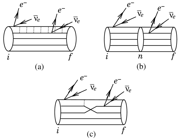
FIG. 1.: a) Diagrams included in the OEM approach. b) General diagram for the Standard and $SU\left(4\right)$ calculation. c) Example of exchange diagram which is not included in the OEM.

FIGURE 1

FIG. 2.: Calculated Gamow-Teller strength for the ${}^{48}Ca\rightarrow^{48}Sc$ transition using the modified Kuo-Brown potential (case a), the modified Bertsh-Hamamoto potential (case b), and the Bertsh-Hamamoto potential (case c). Each histogram represents the total strength in 1 MeV region versus the energy.

FIGURE 2

FIG. 3.: Calculated $\beta^{+}$ strength for the ${}^{48}Ti\rightarrow^{48}Sc$ transition using the modified Kuo-Brown potential (case a), the modified Bertsh-Hamamoto potential (case b), and the Bertsh-Hamamoto potential (case c). Each histogram represents the total strength in 1 MeV region versus the energy.

FIGURE 3

FIG. 4.: Double beta amplitude versus the spin-orbit potential. All curves correspond to the modified B-H potential, except the $M_{{\cal GT}}^{St}$ with squares which corresponds to the B-H potential.

FIGURE 4

FIG. 5.: Detail of the contributions to the double beta amplitude, $M_{{\cal GT}}^{St}$, using the modified Kuo-Brown potential (case a), the modified Bertsh-Hamamoto potential (case b), and the Bertsh-Hamamoto potential (case c). Each histogram represents the total contribution in 1 MeV region versus the energy.

FIGURE 5

REFERENCES

- [1] S. R. Elliot, A. A. Hahn, and M. K. Moe, Phys. Rev. Lett. 59, (1987), 2020; Phys. Rev. C36, (1987), 2129.
- [2] A. Morales, Nucl. Phys. Proc. Suppl. 77, 335 (1999).
- [3] A. Balysh et al., Phys. Rev. Lett., 77, 5186 (1996).
- [4] J. Suhonen and O. Civitarese, Phys. Rep. 300, 123 (1998).
- [5] A. Faessler and F. Šimkovic, J. Phys. G24, 2139 (1998).
- [6] P. Vogel and M. R. Zirnbauer, Phys. Rev. Lett. 57, 3148 (1986).
- [7] J. Engel, P. Vogel, and M. R. Zirnbauer, Phys. Rev. C37, 731 (1988).
- [8] J. G. Hirsch and F. Krmpotić, Phys. Rev. C41, 792 (1990) and J. G. Hirsch, E. Bauer, and F. Krmpotić, Nucl. Phys. A516, 304 (1990).
- [9] J. Bernabeu, B. Desplanques, J. Navarro and S. Noguera, Z. Phys. C46, 323 (1990).
- [10] F. Šimkovic, JINR Rapid communications, 39, 21 (1989); F. Šimkovic and M. Gmitro, Czech. J. Phys. 10, 1105 (1991).
- [11] C. R. Ching and T. H. Ho, Commun. in Theor. Phys. 10, 45 (1988) and 11, 433 (1989). C. R. Ching, T. H. Ho and X. R. Wu, Phys. Rev. C40, 304 (1989).
- [12] M. Hirsch, X. R. Wu, H. V. Klapdor, C. R. Ching, and T. H. Ho, Phys. Rep. 242, 403 (1994).
- [13] See E. Caurier, A. Poves and A. P. Zuker, Phys. Lett. B252, 13 (1990) for the physics discussion and see reference [21] for the final numerical result.
- [14] J. Bernabeu, B. Desplanques and S. Noguera, Z. Phys. C51, 499 (1991).
- [15] J. Engel, W. C. Haxton and P. Vogel, Phys. Rev. C46, 2153 (1992).
- [16] M. Doi, T. Kotani and E. Takasugi, Progr. of Theor. Phys. Suppl. 83, 1 (1985).
- [17] J. G. Hirsch, P. O. Hess and O. Civitarese, Phys. Lett. B390, 36 (1997) and Phys. Rev. C54, 1976 (1996) and C56, 199 (1997).
- [18] B. A. Brown, A. Etchegoyen and W. D. M. Rae, The computer code OXBASH, MSU-NSCL report number 524 (1988). M. Horoi and B. A. Brown Downloading OXBASH from INTERNET, nucl-th/9406020 (1994).
- [19] G. F. Bertsch and I. Hamamoto, Phys. Rev. C26, 1323 (1982).
- [20] L. Zhao, B. A. Brown and W. A. Richter, Phys. Rev. C42, 1120 (1990).
- [21] E. Caurier, A. P. Zuker, A. Poves, and G. Martinez-Pinedo, Phys. Rev. C50, 225 (1994).
- [22] O. A. Rumyantsev and M H. Urin, Phys. Lett. B443, 51 (1998).
- [23] A. Poves, R. P. Bahukutumbi, K. Langanke, P. Vogel, Phys. Lett. B361, 1 (1995).
- [24] G. Röpke, A. Schnell, P. Schuck, U. Lombardo, Phys. Rev. C61, 024306 (2000).
- [25] J. Engel, S. Pittel, P. Vogel, M. Stoitsov and J. Dukelsky, Phys. Rev. C55, 1781 (1997).
- [26] K. Ogawa and H. Horie, Nuclear weak processes and nuclear structure, Eds. M. Morita et al., World Scientific, Singapore 1990.
- [27] Radha et al., Phys. Rev. Lett. 76, 2642 (1996).
- [28] S. Noguera (unpublished): this result is obtained using the method of calculation developed in [9] with the Bersch-Hamamoto potential.
- [29] A. Bouyssy, J.F. Mathiot, Van Giai Nguyen, S. Marcos, Phys. Rev. C36, 380 (1987).