Mid-rapidity charge distribution in peripheral heavy ion collisions

Abstract

The charge density distribution with respect to the velocity of matter produced in peripheral heavy ion reactions around Fermi energy is investigated. The experimental finding of enhancement of mid-rapidity matter shows the necessity to include correlations beyond BUU which was performed in the framework of nonlocal kinetic theory. Different theoretical improvements are discussed. While the in–medium cross section changes the number of collisions, it leaves the transferred energy almost unchanged. In contrast the nonlocal scenario changes the energy transferred during collisions and leads to an enhancement of mid–rapidity matter. The renormalisation of quasiparticle energies can be included in nonlocal scenarios and leads to a further enhancement of mid–rapidity matter distribution. This renormalisation is accompanied by a dynamical softening of the equation of state seen in longer oscillation periods of the excited compressional collective mode. We propose to include quasiparticle renormalisation by using the Pauli–rejected collisions which circumvent the problem of backflows in Landau theory. Using the maximum relative velocity of projectile and target like fragments we associate experimental events with impact parameters of the simulations. For peripheral collisions we find a reasonable agreement between experiment and theory. For more central collisions, the velocity damping is higher in one–body simulations than observed experimentally, because of missing cluster formations in the kinetic theory used.

]

I Introduction

Numerical simulations based either on the Boltzmann equation (including the Pauli blocking it is often called the BUU equation [1]) or on the closely related method of quantum molecular dynamics (QMD) [2, 3] are extensively used to interpret experimental data from heavy ion reactions. Due to their quasi-classical character, they offer a transparent picture of the internal dynamics of reactions and allow one to link observed particle spectra with individual stages of reactions. Naturally, simulation results are only approximate. For example, BUU simulations fail to describe the energy and angular distribution of neutrons and protons in low and mid energy domain [4, 5, 6].

In particular, the formation of a neck–like structure in peripheral heavy ion reactions and the impact on the fragmentation mechanism and production of light charged particles has been discussed for a couple of years [7, 8, 9, 10, 11, 12, 13, 14, 15, 16, 17, 18, 19]. It has been suggested that this neck instability can be important for the fast decomposition of matter and is probably neutron rich [20]. Theoretical investigations suggest that the neck is not formed in usual heavy ion simulations starting from the Landau equation [21, 22, 23] or BUU equations [24, 25] including additional mean field fluctuations derived in [26, 27] and tested [28]. The inclusion of fluctuations in the Boltzmann (BUU) equation has been investigated in [29, 30] resulting in Boltzmann-Langevin pictures [31, 32, 33, 34, 35, 36, 10, 16, 17].

We will take here the point of view that the fluctuations should arise by themselves in a proper kinetic description where all relevant correlations are included in the collision integral. The collision will then cause both a dephasing and fluctuation by itself. This procedure without additional assumption about fluctuations has been given by the nonlocal kinetic theory [37, 38, 39] and applied to heavy ion collisions in [40, 41, 42]. We claim that the derived nonlocal off-set in the collision procedure induces fluctuation in the density and consequently in the mean-field which are similar to the one assumed ad-hoc in the approaches above. As a first step to verify this we will investigate the formation of a neck and the mid–rapidity emission pattern. Indeed as we will demonstrate, the neck is much more pronounced if a nonlocal kinetic theory is used.

Recent INDRA observation shows an enhancement of emitted matter in the region of almost zero relative velocity which means that matter is stopped during the reaction and stays almost at rest [19, 43]. This enhancement of mid–rapidity distribution can possibly be associated with a pronounced neck formation of matter. A pioneering work on describing such mid–rapidity emission has been done by E. Galichet and F. Gulminelli [44]. The main problem is to find a proper selection of experimental data [45]. The comparison between data and simulation has been performed according to cuts in the transverse energy. This was possible since the applied coalescence model allows to get rid of the Fermi motion. Since we want to omit coalescence we select the proper comparison with respect to the maximum velocity of the projectiles with respect to the ratio of transverse to total energy. The latter ratio gives a nearly Fermi motion independent scaling.

We want to investigate here the peripheral heavy ion collisions and want to discuss different theoretical improvements of the BUU simulations. We start from the nonlocal BUU equation which includes from microscopic derivation the effect of binary correlations on the collision process. By this way we obtain a nonlocal off-set of the collision partners which account for the readjustment of the trajectories according to the virial corrections, which would be for hard spheres the excluded volume. This off-set induces mean-field fluctuations similar to the above mentioned improvements of BUU. We will give a combined picture of nonlocal off-sets and quasiparticle renormalisation which leads to the consistent inclusion of binary correlation on the collision integral and mean-field fluctuations. Section II represents the formerly derived nonlocal shifts in terms of an intuitive picture and discusses symmetries and implementation in numerical codes. The quasiparticle renormalisation is suggested in a novel form using the excluded events by Pauli - blocking. In section III we present the numerical results and compare different approximations with the experimental data. Finally in section IV we summarise and give some outlook.

II Theoretical Preliminaries

The need for nonlocal corrections can be stimulated by discussing the scattering of two particles as superpositions of wave packets [46] and similar used in [47]. The asymptotic wave packet after scattering can be written for large distance $x$ from scattering centre

$$\phi^{\rm sc}(x,\kappa_{f},t) = \int{d\kappa\over(2\pi\hbar)^{3}}{\cal F}(x,\kappa,\kappa_{f}){f(\kappa,\cos\theta)\over x}{\rm e}^{i(\kappa x-\epsilon_{\kappa}t)}$$ (1)

with the scattering amplitude $f(\kappa,\cos\theta)$ where $\theta$ is the angle between the relative momenta before, $\kappa$, and after the collision, $\kappa_{f}$. We proceed now and expand the scattering amplitude around the final difference momenta $\kappa_{f}$

$$f(\kappa,\cos\theta)=|f(\kappa,\cos\theta)|{\rm e}^{i\delta(\kappa,\cos\theta)}$$ (2)

$$=f(\kappa_{f},\cos\theta)\left(1+(\kappa-\kappa_{f})\nabla_{\kappa}|f(\kappa,\cos\theta)|_{\kappa=\kappa_{f}}\right)$$ (3)

$$\times{\rm e}^{i(\kappa-\kappa_{f})\nabla_{\kappa}\delta(\kappa,\cos\theta)_{\kappa=\kappa_{f}}}.$$ (4)

The derivative of the phase $\delta$ leads now to the definition of the effective space shifts $\Delta^{f}$ and the time shift $\Delta_{||}$

$$2\Delta^{f} = \nabla_{\kappa}\delta|_{\kappa=\kappa_{f}}={\kappa_{f}\over|\kappa_{f}|}\partial_{\kappa_{f}}\delta+{{\kappa\over|\kappa|}-\cos\theta{\kappa_{f}\over|\kappa_{f}|}\over|\kappa_{f}|}\partial_{\cos\theta}\delta$$ (6)

$$\equiv {\kappa\over m}\Delta_{\|}+({\kappa\over|\kappa|}-\cos\theta{\kappa_{f}\over|\kappa_{f}|})\Delta_{\perp}$$ (7)

where we denoted the shifts corresponding to the direction of $\kappa$ as $\|$ and $\perp$. Rewriting (1) we obtain

$$\phi^{\rm sc}(x,\kappa_{f},t) = {f(\kappa_{f},\cos\theta)\over x}$$ (8)

$$\times \int{d\kappa\over(2\pi\hbar)^{3}}\tilde{\cal F}(x,\kappa,\kappa_{f}){\rm e}^{i\kappa\cdot(x+2\Delta^{f})}{\rm e}^{-i\epsilon_{\kappa}(\Delta_{\|}+t)}.$$ (9)

We observe three effects of scattering on the asymptotics: (i) a genuine time delay $\Delta_{\|}$, (ii) an effective displacement of the two colliding particle of $\Delta^{f}$ with respect to the centre of mass and (iii) a modification of scattering probability $\tilde{\cal F}={\cal F}(1+(\kappa-\kappa_{f})\nabla_{\kappa}|f(p,\cos\theta)|_{\kappa=\kappa_{f}})$.

The effect of non-local collisions on the dynamics of heavy ion reactions has been studied already within a cascade model [48]. For a simple hard-sphere approximation of nucleon-nucleon collisions, Halbert has demonstrated that density patterns of ²⁰Ne$+^{238}$U reactions are sensitive to local or non-local treatment of collisions. Malfliet [49] also found disturbing that all dynamical models rely more or less on the use of the local approximation of binary collisions, because the local approximation neglects a contribution of the collision flux to both material relations which control the hydrodynamic motion during the reaction, the compressibility and the share viscosity. To include the collision flux, Malfliet incorporated hard-sphere non-local collisions into the BUU simulation code. Recently, this approximation has been used by Kortemeyer, Daffin and Bauer [50].

The hard-sphere approximation of a non-local collision is sufficient for the above mentioned discussions of trends, however, it cannot be used in realistic studies. This ad hoc approximation has been used not only for its simplicity but also because of lack of a first principle theory offering quantum mechanical displacements which would generalise the classical hard-sphere displacements proposed by Enskog. As far as we know, till recently there was no non-local theory of binary collisions devoted to the nuclear matter. In literature, there are closely related quantum theories of binary collisions developed for moderately dense gases [51, 52], these, however, treat non-local collisions via gradient contributions to the scattering integral. The gradient form is suitable for hydrodynamic expansions studied in the chemical physics, but is very inconvenient for numerical simulation and thus have never been employed for heavy ion reactions.

Recent theoretical studies have filled this gap in theory. Danielewicz and Pratt [53] pointed out that the collision delay can be used as a convenient tool to describe the virial corrections to the equation of state for the gas of quasiparticles. Although their discussion is limited to the equilibrium, it marks a way how to introduce virial corrections also to dynamical processes. The kinetic equation for quasiparticles with non-instantaneous and non-local scattering integral has been derived in [37, 54] as a systematic quasi-classical limit of non-equilibrium Green’s functions in the Galitskii–Feynman approximation. It has been shown that the gradient corrections to the scattering integral can be rearranged into a form of a collision delay and space displacements reminiscent of classical hard spheres, i.e., into a form suitable for numerical simulations.

In this contribution we will put these ideas of nonlocalities on the firm ground using the quantum kinetic equation with nonlocal scattering integrals which was derived from quantum statistics [37, 54] to show how the effect of nonlocalities play a role in simulations of heavy ion reactions and compare them with experiment.

A Nonlocal kinetic theory

The scattering integral of the non-local kinetic equation derived in [37] corresponds to a following picture of a collision as seen in Figure 1.

FIG. 1.: A nonlocal binary collision according to Eq. (16).

Assume that two particles, $a$ and $b$, of initial momenta $k$ and $p$ start to collide at time instant $t$ being at coordinates $r_{a}$ and $r_{b}$. Due to a finite range of the interaction, at the beginning of collision particles are displaced by $r_{b}-r_{a}=\Delta^{\rm be}$. The collision has a finite duration $\Delta_{t}$, i.e., it ends at $t+\Delta_{t}$. During the collision, both particles move so that their end coordinates differ from those at the beginning, $r_{a}^{\prime}-r_{a}=\Delta_{a}$ and $r_{b}^{\prime}-r_{b}=\Delta_{b}$. The particle $a$ transfers a momentum $q$ to the particle $b$, therefore their relative momentum changes from $\kappa=\frac{1}{2}(k-p)$ to $\kappa^{\prime}=\frac{1}{2}(k-p)-q$. Their sum momentum is modified by an external field acting on the colliding particles during the collision going from $K=k+p$ to $K^{\prime}=k+p+\Delta_{K}$. The same field changes the sum energy of colliding particles from $E=\epsilon_{a}+\epsilon_{b}$ to $E^{\prime}=\epsilon_{a}^{\prime}+\epsilon_{b}^{\prime}=\epsilon_{a}+\epsilon_{b}+\Delta_{E}$.

The values of $\Delta$’s are given by derivatives of the scattering phase shift $\phi={\rm Im\ ln}T_{R}(\Omega,k,p,q,t,r)$,

$$\Delta_{t} = \left.{\partial\phi\over\partial\Omega}\right|_{E},$$ (11)

$$\Delta^{\rm be} = \left({\partial\phi\over\partial p}-{\partial\phi\over\partial q}-{\partial\phi\over\partial k}\right)_{E},$$ (12)

$$\Delta_{a} = \left.-{\partial\phi\over\partial k}\right|_{E},$$ (13)

$$\Delta_{b} = \left.-{\partial\phi\over\partial p}\right|_{E},$$ (14)

$$\Delta_{K} = \left.{\partial\phi\over\partial r}\right|_{E},$$ (15)

$$\Delta_{E} = \left.-{\partial\phi\over\partial t}\right|_{E}.$$ (16)

Note that energy $\Omega$ enters as an independent quantity so that one needs to know the scattering phase shift out of the energy shell. The on-shell energy, $\Omega=E$, is substituted after derivatives are taken. Since experiments provide us only with the on-shell values of the scattering phase shift $\phi$, set (16) of $\Delta$’s cannot be derived directly from experimental values but only indirectly via off-shell T-matrix constructed from the interaction potential. Below we show how to circumvent this complication.

B Instantaneous approximation

It is our intention to incorporate these features of collisions into the BUU (or QMD) simulation codes. The selfconsistent evaluation of all $\Delta$’s for all collisions would be too demanding. We employ two kinds of additional approximations. First we neglect the medium effect on binary collisions, i.e., use the well known free-space T-matrix. Second, we rearrange the scattering integral into an instantaneous but non-local form. This instantaneous form parallels hard-sphere-like collisions what allow us to employ computational methods developed within the theory of gases [55] in a similar way to [50].

In the instantaneous approximation we let particles to make a sudden jump from their in-coming trajectories into their out-going ones so that at time $t+\Delta_{t}$ particles arrive at the correct coordinates, $r_{a}^{\prime}$ and $r_{b}^{\prime}$, with the correct momenta, $\kappa^{\prime}$ and $K^{\prime}$. Accordingly, in the asymptotic region, after $t+\Delta_{t}$, there is no distinction between the non-instantaneous and instantaneous pictures.

The actual time instant at which the jump happens does not influence the asymptotic states, however, two particular choices of the time instant are important with respect to the implementation into simulations. The first one is the time at which the simulation code selects two particles as adepts for the collision usually at the point of closest approach. We will discuss this time later when we specify the simulation scheme. The second one is the central time, $\tilde{t}=t+{1\over 2}\Delta_{t}$, for which the instantaneous approximation maintains the space and time symmetries of the non-instantaneous collision. As we will see, these symmetries allow one to derive the value of the sudden jump from experimental phase shifts.

The condition that the sudden jump correctly mimics the non-instantaneous process is naturally met if one extrapolates the in-coming and out-going trajectories from known coordinates and momenta at $t$ and $t+\Delta_{t}$, respectively, to the central time $\tilde{t}$. Doing so one finds that extrapolated coordinates just before and after the sudden jump read

$$\tilde{r}_{a} = r_{a}+{k\over 2m}\Delta_{t},$$ (17)

$$\tilde{r}_{b} = r_{b}+{p\over 2m}\Delta_{t},$$ (18)

$$\tilde{r}_{a}^{\prime} = r_{a}^{\prime}-{k-q\over 2m}\Delta_{t}=r_{a}+\Delta_{a}-{k-q\over 2m}\Delta_{t},$$ (19)

$$\tilde{r}_{b}^{\prime} = r_{b}^{\prime}-{p+q\over 2m}\Delta_{t}=r_{b}+\Delta_{b}-{p+q\over 2m}\Delta_{t}.$$ (20)

In extrapolations of momenta we neglect Coulomb forces so that we assume that protons and neutrons are driven by the same force from the Skyrme potential $U$, $F=-{\partial U\over\partial r}$. In this case, the relative momentum remains unchanged and the force affects only the sum momentum,

$$\tilde{\kappa} = \kappa,$$ (21)

$$\tilde{K} = K+F\Delta_{t},$$ (22)

$$\tilde{\kappa}^{\prime} = \kappa^{\prime}=\kappa-q,$$ (23)

$$\tilde{K}^{\prime} = K^{\prime}-F\Delta_{t}=K+\Delta_{K}-F\Delta_{t},$$ (24)

Finally, energies at the extrapolated phase-space points are

$$\tilde{\epsilon}_{a} = {\tilde{k}^{2}\over 2m}+U\left(\tilde{r}_{a},t+{\Delta_{t}\over 2}\right)=\epsilon_{a}+{\partial U\over\partial t}{\Delta_{t}\over 2},$$ (25)

$$\tilde{\epsilon}_{b} = {\tilde{p}^{2}\over 2m}+U\left(\tilde{r}_{b},t+{\Delta_{t}\over 2}\right)=\epsilon_{b}+{\partial U\over\partial t}{\Delta_{t}\over 2},$$ (26)

$$\tilde{\epsilon}_{a}^{\prime} = {(\tilde{k}-q)^{2}\over 2m}+U\left(\tilde{r}_{a}^{\prime},t+{\Delta_{t}\over 2}\right)=\epsilon_{a}^{\prime}-{\partial U\over\partial t}{\Delta_{t}\over 2},$$ (27)

$$\tilde{\epsilon}_{b}^{\prime} = {(\tilde{p}+q)^{2}\over 2m}+U\left(\tilde{r}_{b}^{\prime},t+{\Delta_{t}\over 2}\right)=\epsilon_{b}^{\prime}-{\partial U\over\partial t}{\Delta_{t}\over 2}.$$ (28)

In rearrangement we have used that the increase of the kinetic energy, say ${\tilde{k}^{2}\over 2m}-{k^{2}\over 2m}={1\over 2m}\left(k+{1\over 2}F\Delta_{t}\right)^{2}-{k^{2}\over 2m}={kF\over 2m}\Delta_{t}$, is compensated by the decrease of the potential energy along the trajectory, $U(\tilde{r}_{a},t)-U(r_{a},t)={\partial U\over\partial r}{k\over 2m}\Delta_{t}=-F{k\over 2m}\Delta_{t}$. In a stationary potential, the compensation of kinetic and potential energies reflects the energy conservation. The second order corrections in $\Delta$’s are neglected.

Using the extrapolated quantities, we can define a new set of effective $\Delta$’s corresponding to the instantaneous picture,

$$\tilde{\Delta}^{\rm be} = \tilde{r}_{b}-\tilde{r}_{a}=\Delta^{\rm be}-\left({k\over m}-{p\over m}\right){\Delta_{t}\over 2},$$ (29)

$$\tilde{\Delta}_{a} = \tilde{r}_{a}^{\prime}-\tilde{r}_{a}=\Delta_{a}-\left({k-q\over m}+{k\over m}\right){\Delta_{t}\over 2},$$ (30)

$$\tilde{\Delta}_{b} = \tilde{r}_{b}^{\prime}-\tilde{r}_{b}=\Delta_{b}-\left({p+q\over m}+{p\over m}\right){\Delta_{t}\over 2},$$ (31)

The space displacements $\tilde{\Delta}^{\rm be}$, $\tilde{\Delta}_{a}$ and $\tilde{\Delta}_{b}$ can be expressed in terms of the on-shell scattering phase shift defined as

$$\tilde{\phi}(k,p,q,r,t)=\left.\phi\right|_{\Omega={1\over 2}(\epsilon_{a}+\epsilon_{b}+\epsilon_{a}^{\prime}+\epsilon_{b}^{\prime})}.$$ (32)

From (16) and (31) one can directly check that

$$\tilde{\Delta}^{\rm be} = {\partial\tilde{\phi}\over\partial p}-{\partial\tilde{\phi}\over\partial q}-{\partial\tilde{\phi}\over\partial k},$$ (33)

$$\tilde{\Delta}_{a} = -{\partial\tilde{\phi}\over\partial k},$$ (34)

$$\tilde{\Delta}_{b} = -{\partial\tilde{\phi}\over\partial p}.$$ (35)

Effective displacements (35) can be evaluated from the experimentally observed scattering phase shifts. Before we turn to this pragmatic question, it is profitable to enlighten the conservation laws and symmetries of the collision processes.

C Conservation laws

The extrapolated momentum and energy gains vanish,

$$\tilde{\Delta}_{K} = \tilde{K}^{\prime}-\tilde{K}=\Delta_{K}-2F\Delta_{t}=0,$$ (36)

$$\tilde{\Delta}_{E} = \tilde{\epsilon}_{a}^{\prime}+\tilde{\epsilon}_{b}^{\prime}-\tilde{\epsilon}_{a}-\tilde{\epsilon}_{b}=\Delta_{E}-2{\partial U\over\partial t}\Delta_{t}=0.$$ (37)

To show this we use that for a collision of isolated nucleons, the scattering phase shift depends only on the initial and final momenta, $\kappa$ and $\kappa^{\prime}$, while sum momentum $K$ and the Skyrme potential only shifts the energy bottom,

$$\phi(\Omega,k,p,q,r,t)=\phi\left(\Omega-{(k+p)^{2}\over 4m}-2U,k-p,q\right).$$ (38)

The time derivative which results in the energy gain $\Delta_{E}$ thus can be expressed via the energy derivative and from (16) one finds that $\Delta_{E}=2{\partial U\over\partial t}\Delta_{t}$, therefore $\tilde{\Delta}_{E}=0$. The space dependency also enters $\phi$ only via the energy argument, therefore $\Delta_{K}=2F\Delta_{t}$ or $\tilde{\Delta}_{K}=0$. The cancellation of both shifts simplifies the energy and momentum conservation to its form commonly used for instantaneous collisions. Briefly, in the instant collision the Skyrme potential has no time to pass any energy and momentum to colliding nucleons.

An additional simplification follows from the continuity of the centre of mass motion. This requires $\tilde{r}_{a}^{\prime}+\tilde{r}_{b}^{\prime}=\tilde{r}_{a}+\tilde{r}_{b}$ or $\tilde{\Delta}_{a}+\tilde{\Delta}_{b}=0$. This relation is satisfies by displacements (35). Indeed, in the approximation of isolated collision (38), the on-shell energy argument reduces,

$${1\over 2}(\epsilon_{a}+\epsilon_{b}+\epsilon_{a}^{\prime}+\epsilon_{b}^{\prime}) - {(k+p)^{2}\over 4m}-2U$$ (39)

$$= {(k-p)^{2}\over 8m}+{(k-p-2q)^{2}\over 8m}.$$ (40)

The on-shell scattering phase shift (32) then does not depends on the sum momentum $k+p$, therefore the derivatives with respect to $k$ and $p$ are mutually connected,

$${\partial\tilde{\phi}\over\partial k}=-{\partial\tilde{\phi}\over\partial p}.$$ (41)

According to (35), the displacement of the particle $b$ is opposite to the displacement of the particle $a$,

$$\tilde{\Delta}_{b}=-\tilde{\Delta}_{a}.$$ (42)

D Rotational symmetry

The symmetries are best seen in the barycentric representation in which the phase shift is a function of the initial and final relative momenta, $\tilde{\phi}(k-p,q)\equiv\tilde{\phi}(\kappa,\kappa^{\prime})$, where $\kappa={1\over 2}(k-p)$ and $\kappa^{\prime}={1\over 2}(k-p-2q)$. From substitution into the barycentric framework one obtains

$${\partial\over\partial k} = {\partial\kappa\over\partial k}{\partial\over\partial\kappa}+{\partial\kappa^{\prime}\over\partial k}{\partial\over\partial\kappa^{\prime}}={1\over 2}{\partial\over\partial\kappa}+{1\over 2}{\partial\over\partial\kappa^{\prime}}$$ (43)

$${\partial\over\partial p} = {\partial\kappa\over\partial p}{\partial\over\partial\kappa}+{\partial\kappa^{\prime}\over\partial p}{\partial\over\partial\kappa^{\prime}}=-{1\over 2}{\partial\over\partial\kappa}-{1\over 2}{\partial\over\partial\kappa^{\prime}}$$ (44)

$${\partial\over\partial q} = {\partial\kappa\over\partial q}{\partial\over\partial\kappa}+{\partial\kappa^{\prime}\over\partial q}{\partial\over\partial\kappa^{\prime}}=-{\partial\over\partial\kappa^{\prime}},$$ (45)

therefore the displacements in terms of relative momenta read

$$\tilde{\Delta}_{a} = -{1\over 2}{\partial\tilde{\phi}\over\partial\kappa}-{1\over 2}{\partial\tilde{\phi}\over\partial\kappa^{\prime}},$$ (46)

$$\tilde{\Delta}^{\rm HS} = \tilde{\Delta}_{b}+\tilde{\Delta}^{\rm be}=\tilde{\Delta}^{\rm be}-\tilde{\Delta}_{a}$$ (47)

$$= -{1\over 2}{\partial\tilde{\phi}\over\partial\kappa}+{1\over 2}{\partial\tilde{\phi}\over\partial\kappa^{\prime}}.$$ (48)

Apparently, the $\tilde{\Delta}_{a}$ does not change under replacement of the initial and final momenta, $\kappa\longleftrightarrow\kappa^{\prime}$. As a complementary displacement we have introduced $\tilde{\Delta}^{\rm HS}$ instead of $\tilde{\Delta}^{\rm be}$ which reverses its orientation under the replacement of initial and final momenta.

For central forces, the scattering phase shift has to satisfy the rotational symmetry, therefore it depends only on the deflection angle $\theta$

$$\cos\theta={\kappa\kappa^{\prime}\over|\kappa||\kappa^{\prime}|}$$ (49)

and amplitudes of initial and final relative momenta,

$$\tilde{\phi}(\kappa,\kappa^{\prime})=\tilde{\phi}(\cos\theta,|\kappa|,|\kappa^{\prime}|).$$ (50)

The vector derivatives follow from ${\partial\over\partial\kappa}\cos\theta=\kappa^{\prime}{1\over|\kappa||\kappa^{\prime}|}-\kappa{\cos\theta\over|\kappa|^{2}}$ and ${\partial\over\partial\kappa}|\kappa|={\kappa\over|\kappa|}$ as

$${\partial\tilde{\phi}\over\partial\kappa}=\kappa\left({1\over|\kappa|}{\partial\tilde{\phi}\over\partial|\kappa|}-{\cos\theta\over|\kappa||\kappa^{\prime}|}{\partial\tilde{\phi}\over\partial\cos\theta}\right)+\kappa^{\prime}{1\over|\kappa||\kappa^{\prime}|}{\partial\tilde{\phi}\over\partial\cos\theta}.$$ (51)

The derivative with respect to the final momentum $\kappa^{\prime}$ is obtained from (51) via the interchange $\kappa\longleftrightarrow\kappa^{\prime}$.

E Time-reversal symmetry

As mentioned above, we want to express the effective displacements in terms of observable scattering phase shifts. This will make possible to circumvent the uncertainty about interaction potentials and to supply the simulation codes directly with experimental values.

Although the phase shift $\tilde{\phi}$ does not depend on the energy $\Omega$, it is still not experimentally known for general momentum $q$ but only for momenta which satisfy the energy conservation, $(k-p)^{2}=(k-p-2q)^{2}$. Due to time-reversal symmetry of the collision process, it is possible to express the effective displacements in terms of derivatives along this momentum shell.

The experimentally available values of the scattering phase shift are restricted to the shell $|\kappa^{\prime}|=|\kappa|$,

$$\phi_{\rm exp}(\cos\theta,|\kappa|)=\left.\tilde{\phi}(\cos\theta,|\kappa|,|\kappa^{\prime}|)\right|_{|\kappa^{\prime}|=|\kappa|}.$$ (52)

In (51) we need separate derivations with respect to $|\kappa|$ and $|\kappa^{\prime}|$. Fortunately, due to the time and space reversal symmetries, the scattering phase shift is a symmetric function of $|\kappa|$ and $|\kappa^{\prime}|$,

$$\tilde{\phi}(\cos\theta,|\kappa|,|\kappa^{\prime}|)=\tilde{\phi}(\cos\theta,|\kappa^{\prime}|,|\kappa|).$$ (53)

Since we need to find the derivatives only for $|\kappa^{\prime}|=|\kappa|$ and symmetry (53) implies

$$\left.{\partial\over\partial|\kappa^{\prime}|}\tilde{\phi}(|\kappa|,|\kappa^{\prime}|)\right|_{|\kappa^{\prime}|=|\kappa|}=\left.{\partial\over\partial|\kappa|}\tilde{\phi}(|\kappa|,|\kappa^{\prime}|)\right|_{|\kappa^{\prime}|=|\kappa|}$$ (54)

we obtain a direct link to observable scattering phase shift

$$\left.{\partial\over\partial|\kappa^{\prime}|}\tilde{\phi}(\cos\theta,|\kappa|,|\kappa^{\prime}|)\right|_{|\kappa^{\prime}|=|\kappa|}={1\over 2}{\partial\over\partial|\kappa|}\phi_{\rm exp}(\cos\theta,|\kappa|).$$ (55)

F Displacements in simulations

Now we are ready to evaluate the effective displacements from experimental scattering phase shifts. From (48), (51) and (55) we find

$$\tilde{\Delta}_{a} = -{\kappa+\kappa^{\prime}\over 2|\kappa|^{2}}\left({|\kappa|\over 2}{\partial\phi_{\rm exp}\over\partial|\kappa|}-\left(\cos\theta-1\right){\partial\phi_{\rm exp}\over\partial\cos\theta}\right),$$ (56)

$$\tilde{\Delta}^{\rm HS} = -{\kappa-\kappa^{\prime}\over 2|\kappa|^{2}}\left({|\kappa|\over 2}{\partial\phi_{\rm exp}\over\partial|\kappa|}-\left(\cos\theta+1\right){\partial\phi_{\rm exp}\over\partial\cos\theta}\right).$$ (57)

In agreement with their even/odd symmetry under interchange of initial and final momenta, the $\tilde{\Delta}_{a}$ is proportional to the sum $\kappa+\kappa^{\prime}$ while $\tilde{\Delta}^{\rm HS}$ to the difference $\kappa+\kappa^{\prime}$. From the energy conservation, $(\kappa+\kappa^{\prime})(\kappa-\kappa^{\prime})=\kappa^{2}-\kappa^{\prime 2}=0$, follows that these two vectors are orthogonal. Before we present actual values of displacements, it is profitable to compare their form with the model of hard spheres and the approximation by the collision delay.

For classical hard spheres of radius $R$, the scattering phase shift depends only on the transferred momentum $q=\kappa-\kappa^{\prime}$ as, $\phi^{\rm HS}=\pi-2|q|R$. From (57) than follows that $\tilde{\Delta}_{a}=0$ and $\tilde{\Delta}^{\rm HS}={q\over|q|}2R$. The hard-sphere approximation used in model studies [48, 49, 50] thus neglects $\tilde{\Delta}_{a}$ and uses a constant approximation of the amplitude of the other displacement, $\left|\tilde{\Delta}^{\rm HS}\right|=2R$. This amplitude is conveniently evaluated from the cross section, $\sigma=\pi R^{2}$.

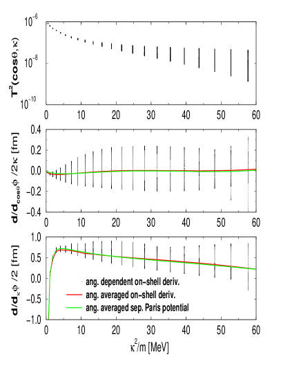
FIG. 2.: The effective displacement as a function of the deflection angle and the kinetic energy, $\kappa^{2}/m$, in the barycentric coordinate system. The columns of dots show the spread of components with deflection angle. The lines show the angle-averaged values. The amplitude of the T-matrix is presented in the top section to indicate the weight of individual processes. The orthogonal component, $\overline{\Delta_{\perp}}/2\equiv d\phi/d{\cos\theta}/2\kappa$ shown in the middle section, has appreciably smaller values than the parallel component, $\overline{\Delta_{\|}}/2m\equiv d\phi/d\kappa/2$ shown in the bottom section.

The approximation discussed by Danielewicz and Pratt [53] deals only with the collision delay defined according to Wigner as the energy derivative of the scattering phase shift. This approximation is obtained from (57) if one neglects the derivative with respect to the deflection angle, therefore $\tilde{\Delta}_{a}=-{\kappa+\kappa^{\prime}\over 2m}{\partial\phi_{\rm exp}\over\partial E}$ and $\tilde{\Delta}^{\rm HS}=-{\kappa-\kappa^{\prime}\over 2m}{\partial\phi_{\rm exp}\over\partial E}$, where $E=|\kappa|^{2}/m$ is energy in the barycentric system.

Numerical values of these two contributions are compared in Fig. 2. The dots in the vertical line show a spread of values due to the angular dependence, the curves show values averaged over deflection angles with the weight given by the differential cross section displayed in the top section. The parallel component, shown in the bottom section, has a typical value of 0.5 fm. The negative large values below 3 MeV can be ignored since corresponding processes have very small rates due to the Pauli blocking. The perpendicular component, shown in the middle section, has about three-times smaller values, moreover it tends to average out. For energies above $10$MeV, the displacements can be well approximated by a constant value, as it is case of the hard-sphere model. Moreover, the amplitude of the displacement is close to the estimate based on the differential cross section, in spate conceptual difference between both concepts. Our results thus confirm that estimates used in [48, 49, 50, 53] are quite reasonable.

In [38] we have used as the time of instant jump the time of closest approach. This distance is different from the distance $\Delta^{\rm be}$ required from the equivalent scattering scenario presented in figure 3 as solid line.We consider now the time required to travel from $\Delta_{\rm be}$ to the distance of closest approach $\tilde{\Delta}_{t}={m\over 2\kappa^{2}}\kappa\Delta_{\rm be}$ in analogy to [56]. Within this scenario we are allowed to jump at the point of closest approach to the final asymptotics (20) and (24)with the additional distance the particle travel during $\tilde{\Delta}_{t}$. The effective final jump in the barycentric frame is

$$\Delta^{f} = \frac{1}{2}(\Delta_{a}-\Delta_{b}-\Delta^{\rm be})-{\kappa^{\prime}\over m}(\Delta_{t}-\tilde{\Delta}_{t})$$ (58)

$$= \frac{1}{2}(\tilde{\Delta}_{a}-\tilde{\Delta}^{\rm HS})+{\kappa^{\prime}\over 2|\kappa|^{2}}\kappa\cdot(\tilde{\Delta}_{a}+\tilde{\Delta}^{\rm HS})$$ (59)

where the same compensation of off-shell derivatives by $\Delta_{t}$ occurs as described before when jumping at the centre time $\tilde{t}$. Please remark that (59) agrees with (7).

FIG. 3.: A nonlocal binary collision (solid line) together with the scenario of sudden jump at the closest approach.

G Renormalisation of quasiparticle energies

So far we have discussed the nonlocal shifts as if there were free classical particles. The interaction affects, however, the free motion of particles between individual collisions. The dominant effect is due to mean-field forces which bind the nucleus together, accelerating particles close to the surface towards the centre. These forces are conveniently included via potentials of Skyrme and Hartree type.

Beside forces, the interaction also modifies the velocity with which a particle of a given momentum propagates in the system. This effect is known as the mass renormalisation. A numerical implementation of the renormalised mass is rather involved since a plain use of the renormalised mass instead of the free one leads to incorrect currents. Within the Landau concept of quasiparticles, this problem is cured by the back flow, but it is not obvious how to implement the back flow within the BUU simulation scheme. In our studies, we circumvent the problem of back flows using explicit zero-angle collisions to which we add a non-local correction.

1 One-dimensional system of fixed scatterers

A link between the renormalisation of the mass and zero-angle collision has been already pointed out by Landau. We find it instructive to describe this mechanism first for a simple one-dimensional system of randomly distributed barriers. Tunnelling then corresponds to the zero-angle scattering and reflection to a dissipative collision. We focus on the piece of quasi-free trajectory, i.e., the trajectory between two successive dissipative collisions.

A tunnelling through barriers speeds up or slow down the mean velocity of particles. To simulate this effect on the motion, at each tunnelling we shift a particle by a displacement $D$ in the direction of its motion. For simplicity we take the amplitude of $D$ as constant. After time $t$ the particle moves over a distance

$$x=t{k\over m}+N\,D,$$ (60)

where $k/m$ is its velocity between tunnellings and $N$ is the number of barriers on the trajectory of length $x$. In average $N=cx$, where $c$ is concentration of barriers. The mean velocity of a particle then reads

$$v={x\over t}={k\over m}+cD{x\over t}={k\over m(1-cD)}\approx{k\over m}(1+cD).$$ (61)

For the three-dimensional system with particle-particle interactions, the corrections to the mean velocity will be limited to the linear approximation.

Relation (61) can be compared with the velocity of a particle evaluated within the renormalised mass $m^{*}$,

$$v={k\over m^{*}},$$ (62)

from which follows

$${m\over m^{*}}=1+cD.$$ (63)

We can use (63) to fit $D$ so that the known renormalised mass $m^{*}$ is reproduced.

2 Three-dimensional Fermi liquid

In the classical three-dimensional system all collisions have a finite deflection angle. In the quantum system, however, there are zero-angle collisions which represent an interference between scattering states and the incoming state of the interaction. In the dialect of the perturbative expansion one can say that the particle makes a detour from its trajectory in the phase space but nowhere on the detour it reaches the energy shell and thus it has to return back. The detour causes a delay expressed by the shift $D$. In the Fermi liquid, the Pauli exclusion principle blocks a majority of phase space cell on the energy shell so that the zero-angle collisions dominate over the dissipative events. We will use these blocked events to simulate the renormalisation of the mass.

Unlike in the simple one-dimensional scattering on fixed defects, the displacement $D$ is a vector oriented along the difference momentum,

$$D=|D|{k-p\over|k-p|},$$ (64)

where $k$ is a momentum of the assumed particle while $p$ belongs to its partner in the prohibited collision. In general, the displacement $|D|$ is a function of $k$ and $p$. For simplicity we assume this function as a constant and fit its value to the mass renormalisation at the Fermi surface.

For the fitting of the displacement $D$ we assume the zero temperature at which all real collisions are blocked by the Pauli exclusion principle so that all binary encounters contribute to the renormalisation. The mean velocity of the particle is then given by its free motion and the mean value of the displacements per the time unit,

$$v={k\over m}+\sum_{a}\int{dp\over(2\pi\hbar)^{3}}\sigma{|k-p|\over m}f_{p}|D|{k-p\over|k-p|}.$$ (65)

The mean value of displacements is proportional to the frequency of binary entertainments, i.e., it is the sum of integrals over distributions of protons and neutrons weighted with the scattering cross section $\sigma$ and their relative velocity to the observed particle.

With a good approximation the cross section $\sigma$ is independent of energy so that one can easily evaluate the integral in (65),

$$v={k\over m}+n\sigma|D|{k\over m}-n\sigma|D|\langle v\rangle.$$ (66)

The renormalised velocity thus depends on the density,

$$n=\sum_{a}\int{dp\over(2\pi\hbar)^{3}}f_{p}={2p_{F}^{3}\over 3\pi^{2}\hbar^{3}},$$ (67)

and the mean velocity of the nuclear matter,

$$\langle v\rangle={1\over n}\sum_{a}\int{dp\over(2\pi\hbar)^{3}}f_{p}{p\over m}.$$ (68)

For the system in rest, $\langle v\rangle=0$, we find the mass renormalisation,

$${m\over m^{*}}=1+n\sigma|D|.$$ (69)

One can see that this formula has the same interpretation as the one-dimensional case (63), because $n\sigma$ is the average number of scatterers on the trajectory of unitary length.

Formula (69) allows us to fit $|D|$ from known value of the effective mass. For $m^{*}:m=3:4$, $\sigma=40$ mb and $n=0.16$ fm^-3 one finds value $|D|=0.5$ fm. This value is very close to the nonlocal correction in dissipative collisions, see Fig. 2.

The quasiparticle velocity (66) relates to the quasiparticle energy by $v=\partial\epsilon_{k}/\partial k$. For the moving nuclear matter $\langle v\rangle\neq 0$ one finds

$$\epsilon_{k}={k^{2}\over 2m}+n\sigma|D|{(k-m\langle v\rangle)^{2}\over 2m}.$$ (70)

An approximation of this structure is commonly used in simple applications of the Landau concept of quasiparticles.

H Summary an simulation schema

The derived effective nonlocal collision procedure is easily incorporated in the usual collision simulation by an additional advection step. The quasiparticle renormalisation and effective mass is found to be possible to incorporate by the same advection step but performed for the events rejected normally by Pauli-blocking.

Finally, we would like to comment on properties of the proposed simulation scheme. The renormalisation depends on the distribution of particles in surrounding medium. It has four nice properties: (i) the renormalisation vanishes as the local density goes to zero, (ii) the renormalisation vanishes when a high temperature closes the Luttinger gap because all collisions will be at finite angles, (iii) the anisotropy of the quasiparticle velocity in a presence of a non-zero current in medium is automatically covered, and (iv) the backflows connected to the mass renormalisation are covered because both particles jump keeping the centre of mass fixed. Last but not least, the simulation does not require to introduce new time-demanding procedures, one can simply use the scattering events which are merely rejected in standard simulation codes by Pauli-blocking.

III Numerical results

Let us discuss the proposed correction to the local and ideal (no quasiparticle renormalisation) Boltzmann (BUU) simulation. First we introduce the pure nonlocal corrections and then we discuss the quasiparticle renormalisation.

The evolution of the density can be seen in the corresponding left pictures of figure 4 for the BUU (left panel) and nonlocal scenario (middle panel) as well as the additional quasiparticle renormalisation (right panel). We see that the nonlocal scenario leads to a longer and more pronounced neck formation between $200-240$fm/c while the BUU breaks apart already at $200$fm/c.

The question arises whether this pronounced neck formation is simply by more collisions and corresponding correlations. This would lead us to the assumption that a simply increase in the cross section as sometimes called in–medium effect would lead to the mid–rapidity matter enhancement. This is however only the case for smaller impact parameters [44]. To understand the qualitative difference between the nonlocal scenario and an increase of cross section by in–medium effects we perform a simulation where in the local BUU scenario the cross section has been doubled. We see in in the next figure 5 the number of collisions per time for the different scenarios.

FIG. 4.: The time evolution of ${}^{181}_{73}Ta+^{197}_{79}Au$ collisions at $E_{lab}/A=33$ MeV and $8$fm impact parameter in the BUU (left), nonlocal kinetic model (middle) as well as the nonlocal model with quasiparticle renormalisations (right). Plots in the first column show the $(x-z)$ - density cut where $Ta$ as projectile comes from below. The mass momenta are shown by arrows. The corresponding second column gives the charge density distribution versus relative velocity in $cm/ns$ where the target like distribution of $Au$ is on the left and the projectile like distributions of $Ta$ on the right.

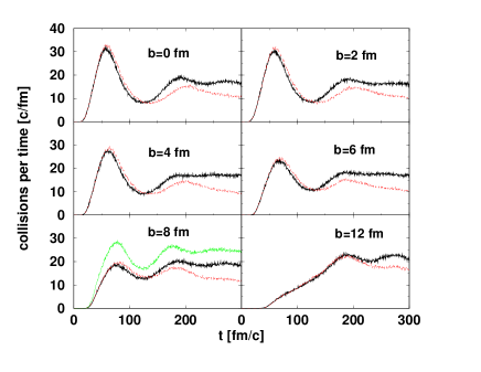
FIG. 5.: The time evolution of the number of nucleon collisions for $Ta+Au$ at $E_{lab}/A=33$ MeV and different impact parameter in the BUU (thick black line), nonlocal kinetic model (broken line) and for the case of $8$fm impact parameter the local BUU with a cross section twice as large (thin dark line).

For $8$ fm impact parameter we compare the local BUU (thick black line) with the nonlocal (broken line) and the local BUU multiplying the cross section with two(thin line). We see that the number of collisions are visibly enhanced by doubling the cross section while for the nonlocal scenario we get only a slight enhancement at the beginning and later even lower values with respect to local BUU. The latter fact comes from the earlier decomposition of matter in the nonlocal scenario. Consequently from the number of collisions we would conclude that the increase of cross section leads to more correlations than the nonlocal scenario.

However when we look at the corresponding transverse and kinetic energies in figure 6 ($8$fm impact parameter) we see that the transverse and longitudinal energy is almost not changed compared with local BUU. Oppositely the nonlocal scenario leads to an increase of transverse energy of about $2$MeV and about $1$MeV in longitudinal energy. We conclude that the increase of cross section leads to a higher number of collisions but not to more dissipated energy while the nonlocal scenario does not change the number of collisions much but the energy dissipated during the collisions. Roughly speaking we can say that the quality of collision is changed.

Returning to the discussion of pronounced neck formation in figure 4 above we see now that the quality rather than the quantity of collisions is what produces the neck. The simple increase of the number of collision does not change much.

Now we can proceed and discuss the charge matter distribution with respect to the velocity. We evaluate the mean density and velocity,

$$n(r,t) = \int{dp\over(2\pi)^{3}}f(p,r,t)$$ (71)

$$v(r,t) = \frac{1}{m\,n(r,t)}\int{dp\over(2\pi)^{3}}pf(p,r,t),$$ (72)

from which we define the distribution of hydrodynamical velocities

$$F({\bar{v}},t)=\int dr\,n(r,t)\,\delta({\bar{v}}-v_{\rm fiss}(r,t))$$ (73)

where $v_{\rm fiss}(r,t)$ is the projection of $v(r,t)$ onto the fission line. This distribution we identify with the so called charge density distribution.

The definition of mean mass (current) velocity does not include the Fermi energy which is integrated out. In the case that we do have a different repartitioning of Fermi energy during the collision than described in our kinetic equation we will have here an ambiguity. Since the dynamical cluster formation is not described in our approach we might have here a smaller effect of Fermi energy on the mass velocity. This will lead us indeed to the observation that BUU or nonlocal kinetic equations have too much stopping compared to the experiment when more central collisions are considered. For peripheral collisions we believe that this kinetic description is sufficient which we will prove by proper association of experimental events to the maximum in the velocity distribution.

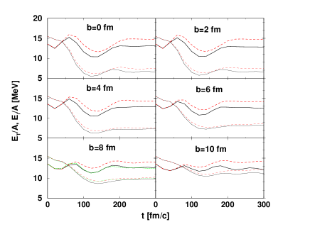
FIG. 6.: The time evolution of the longitudinal (thin lines) and transverse energy (thick lines) including Fermi motion of nucleon collisions for $Ta+Au$ at $E_{lab}/A=33$ MeV and different impact parameter in the BUU (black line), nonlocal kinetic equation (dashed line) and for the case of $8$fm impact parameter the local BUU but with twice the cross section (dotted line).

We plot in figure 4 also the normalised charge distribution versus velocity and see that after $160$fm/c we have an appreciable higher mid–rapidity distribution for the nonlocal scenario (mid panel) than the BUU (left panel). Together with the observation that for nonlocal scenario we have a pronounced neck formation we see indeed that the neck formation is accompanied with high mid-velocity distribution of matter.

A Quasiparticle renormalisation

Now we use the quasiparticle renormalisation schema which has been outlined in chapterII G. We see in figure 4 (right panel) that the mid–rapidity distribution of matter is once more enhanced in comparison to nonlocal scenario without quasiparticle renormalisation. The seemingly shorter lifetime of the neck is artificial due to the chosen density contours which means we have lower densities and faster matter disintegration so that in fact the neck is much more pronounced than in simple nonlocal scenario and of course more pronounced than in BUU. The detailed comparison of the time evolutions of the transverse energy for $8$fm impact parameter can be seen in figure 7.

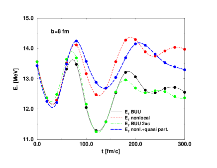
FIG. 7.: The time evolution of the transverse energy including Fermi motion for $Ta+Au$ at $E_{lab}/A=33$ MeV and $8$fm impact parameter in the BUU (black line), nonlocal kinetic equation (dashed line), the local BUU but twice cross section (dashed dotted line) and the nonlocal scenario with quasiparticle renormalisation (long dashed line).

We recognise that the transverse energies including quasiparticle renormalisation are similar to the nonlocal scenario and higher than the BUU or BUU with twice the cross section. However please remark that the period of oscillation in the transverse energy which corresponds to a giant resonance becomes larger for the case with quasiparticle renormalisation. Since therefore the energy of this resonance decreases we can conclude that the compressibility has been decreased by the quasiparticle renormalisation. Sometimes this quasiparticle renormalisation have been introduced by momentum dependent mean-fields. The effect is known to soften the equation of state. We see here that we get a dynamical quasiparticle renormalisation and a softening of equation of state. This softening of equation of state is already slightly remarkable when the nonlocal scenario is compared with BUU. With additional quasiparticle renormalisation we see that this is much pronounced.

B Comparison with experiments

The BUU simulations will now be compared to one experiment performed with INDRA at GANIL, the $Ta+Au$ collision at $E_{lab}/A=33$ MeV. The first question when comparing with experiments concerns the proper selection of events such that one can compare with specific impact parameter of the simulation. We choose here the point of view that the maximum in the charge distribution with respect to velocity which is a measure for stopping gives a good correlation with impact parameter. Indeed if we compare the corresponding correlation between impact parameter and this maximum velocity we obtain indeed an almost linear correlation as in figure 8.

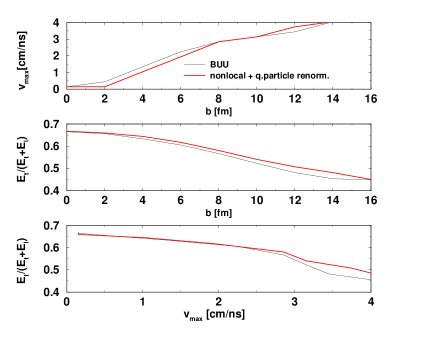
FIG. 8.: The maximum velocity, impact parameter and ratio of longitudinal to total kinetic energy of $Ta+Au$ collisions at $E_{lab}/A=33$ MeV in the BUU (solid line) and the nonlocal model with quasiparticle renormalisation (dotted line).

The matter distribution is shown for different approximations in figure 9. One recognises clearly the successive enhancement of mid–rapidity matter around $6-8$fm if one uses nonlocal kinetic theory and quasiparticle renormalisation correspondingly. It is interesting to remark that the dynamical quasiparticle renormalisation which leads to a softening of the equation of state as discussed in figure 7 enhances the mid rapidity distribution. In contrast a mere soft static parametrisation of the mean-field does not change the mid-rapidity emission appreciably [44].

For the identification with experimental selection we use the selection of events in the following way. First we select events which show a clear one fragment structure. This correspond to events where we have clear target and projectile like residues. Since the used kinetic theory is not capable to describe dynamical fragment formation we believe that these events are the one which are at least describable within our frame. Next we use impact parameter cuts with respect to the transverse energy since this shows in all simulation a fairly good correlation to the impact parameter. In our numerical results we see almost linear correlations between impact parameter, maximal velocity and the convenient ratio between transverse and total kinetic energy as seen in figure 8.

For each selected experimental transverse energy bin we can plot now the maximum velocity versus the ratio of the transverse to kinetic energy. We see in figure 10 that the numerical velocity damping agrees with the experimental selection only for very peripheral collisions. For such events we plot in the figure 10 the charge density distribution and compare the experiment with the simulation. These charge density distributions have been obtained using the procedure described in reference [45]. The Data are represented by light grey points, the standard BUU calculation by the thin line and the non-local BUU with quasiparticle renormalisation calculation by the thick line. A reasonable agreement is found for the nonlocal scenario including quasiparticle renormalisation while simple BUU fails to reproduce mid–rapidity matter.

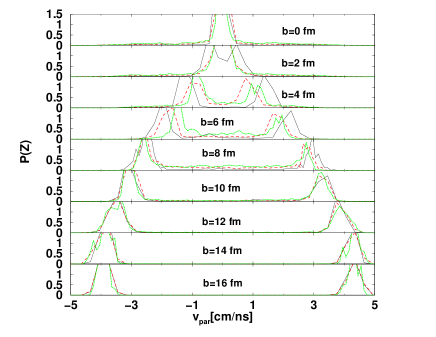
FIG. 9.: The matter distribution versus velocity of $Ta+Au$ collisions at $E_{lab}/A=33$ MeV and different impact parameter in the BUU (solid line), nonlocal kinetic equation (dashed line) as well as the nonlocal model with quasiparticle renormalisation (dotted line).

IV Summary and conclusion

The extension of BUU simulations by nonlocal shifts and quasiparticle renormalisation has been presented and compared to recent experimental data on mid rapidity charge distributions. It is found that both the nonlocal shifts as well as the quasiparticle renormalisation must be included in order to get the observed mid–rapidity matter enhancement.

The inclusion of quasiparticle renormalisation has been performed by using the normally excluded events by Pauli blocking. Since the quasiparticle renormalisation and corresponding effective mass features can be considered as zero angle collisions they can be realized by nonlocal shifts for the scattering events which are normally rejected. This means that one has to perform the advection step for the cases of Pauli blocked collisions without colliding the particles. Besides giving a better description of experiments, this has the effect of a dynamically softening of equation of state seen in longer oscillations of giant compressional resonance.

In this way we present a combined picture including nonlocal off-sets representing the nonlocal character of scattering, which leads to virial correlations with the quasiparticle renormalisation, and as a result to mean field fluctuations. We propose that no additional stochasticity need to be assumed in order to get realistic fluctuations.

V Acknowledgements

The authors would like to thank the members of the INDRA collaboration for providing the experimental data. N. Shannon is thanked for reading the manuscript.

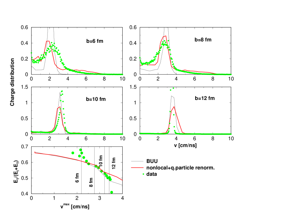
FIG. 10.: The experimental charge distribution of matter (dotted line) versus velocity in comparison with in the BUU (thin solid line) and the nonlocal model with quasiparticle renormalisation (thick line). The maximum velocity versus ratio of longitudinal to total kinetic energy of $Ta+Au$ collisions at $E_{lab}/A=33$ MeV is given below. The selected experimental cuts are given by dots.

REFERENCES

- [1] G. F. Bertsch and S. D. Gupta, Phys. Rep. 160, 189 (1988).
- [2] H. Stöcker and W. Greiner, Phys. Rep. 137, 277 (1986).
- [3] J. Aichelin, Phys. Rep. 202, 235 (1991).
- [4] J. Tõke and et. al., Phys. Rev. Lett. 75, 2920 (1995).
- [5] S. Baldwin and et. al., Phys. Rev. Lett. 74, 1299 (1995).
- [6] W. Skulski and et. al., Phys. Rev. C 53, R2594 (1996).
- [7] L. Stuttgé and et al., Nucl. Phys. A 539, 511 (1992).
- [8] G.Casini and et al., Phys. Rev. Lett. 71, 2567 (1993).
- [9] C.P.Montoya and et al., Phys. Rev. Lett. 73, 3070 (1994).
- [10] M. Colonna, M. D. Toro, and A. Guarnera, Nucl. Phys. A 589, 160 (1995).
- [11] J. F. Lecolley and et al., Phys. Lett. B 354, 202 (1995).
- [12] J. Tõke and et al., Nucl. Phys. A 583, 519 (1995).
- [13] A. A. Stefanini, Zeit. für Phys. A 351, 167 (1995).
- [14] J.F.Dempsey and et al., Phys. Rev. C 54, 1710 (1996).
- [15] S.L.Chen and et al., Phys. Rev. C 54, 2214 (1996).
- [16] M. Colonna et al., Nucl. Phys. A 642, 449 (1998).
- [17] G. Fabbri, M. Colonna, and M. D. Toro, Phys. Rev. C 58, 3508 (1998).
- [18] Y. Larochelle and et al., Phys. Rev. C 59, 565 (1999).
- [19] F. Bocage and et al., Nucl. Phys. A 676, 391 (2000).
- [20] L. G. Sobotka, J. F. Dempsey, R. J. Charity, and P. Danielewicz, Phys. Rev. C 55, 2109 (1997).
- [21] C. Pethik and D. Ravenhall, Nucl. Phys. A 471, 19c (1987).
- [22] R. Donangelo, C. O. Dorso, and H. D. Marta, Phys. Lett. B 263, 19 (1991).
- [23] R. Donangelo, A. Romanelli, and A. C. S. Schifino, Phys. Lett. B 263, 342 (1991).
- [24] D. Kiderlen and H. Hofmann, Phys. Lett. B 332, 8 (1994).
- [25] S. Ayik, M. Colonna, and P. Chomaz, Phys. Lett. B 353, 417 (1995).
- [26] R. Balian and M. Veneroni, Ann. of Phys. 164, 334 (1985).
- [27] H. Flocard, Ann. of Phys. 191, 382 (1989).
- [28] T. Troudet and D. Vautherin, Phys. Rev. C 31, 278 (1985).
- [29] S. Chattopadhyay, Phys. Rev. C 52, R480 (1995).
- [30] S. Chattopadhyay, Phys. Rev. C 53, 1065 (1996).
- [31] E. Suraud, S. Ayik, J. Stryjewski, and M. Belkacem, Nucl. Phys. A 519, 171c (1990).
- [32] S. Ayik and C. Gregoire, Nucl. Phys. A 513, 187 (1990).
- [33] J. Randrup and B. Remaud, Nucl. Phys. A 514, 339 (1990).
- [34] S. Ayik, E. Suraud, M. Belkacem, and D. Boilley, Nucl. Phys. A 545, 35 (1992).
- [35] M. Colonna et al., Phys. Rev. C 47, 1395 (1993).
- [36] M.Colonna, Ph.Chomaz, and J.Randrup, Nucl.Phys. A 567, 637 (1994).
- [37] V. Špička, P. Lipavský, and K. Morawetz, Phys. Lett. A 240, 160 (1998).
- [38] K. Morawetz et al., Phys. Rev. Lett. 82, 3767 (1999).
- [39] P. Lipavský, V. Špička, and K. Morawetz, Phys. Rev. E 59, R 1291 (1999).
- [40] K. Morawetz, P. Lipavský, V. Špička, and N. Kwong, Phys. Rev. C 59, 3052 (1999).
- [41] K. Morawetz, Phys. Rev. C 62, 44606 (2000).
- [42] K. Morawetz, S. Toneev, and M. Ploszajczak, Phys. Rev. C 62, 64602 (2000).
- [43] E. Plagnol and et al., Phys. Rev. C 61, 014606 (2000).
- [44] E. Galichet, Ph.D. thesis, Insitut de Physique Nucléaire de Lyon, 1998.
- [45] J. Lecolley and et al., Nucl. Inst. and Meth. A 441, 517 (2000).
- [46] V. Špička, P. Lipavský, and K. Morawetz, Phys. Rev. B 55, 5084 (1997).
- [47] J. Aichelin and C. Hartnack, in Proceedings of the international workshop (GSI, Hirschegg, Kleinwalsertal, 1997), p. 416.
- [48] E. C. Halbert, Phys. Rev. C 23, 295 (1981).
- [49] R. Malfliet, Nucl. Phys. A 420, 621 (1983).
- [50] G. Kortemeyer, F. Daffin, and W. Bauer, Phys. Lett. B 374, 25 (1996).
- [51] P. J. Nacher, G. Tastevin, and F. Laloe, Ann. Phys. (Leipzig) 48, 149 (1991).
- [52] M. de Haan, Physica A 164, 373 (1990).
- [53] P. Danielewicz and S. Pratt, Phys. Rev. C 53, 249 (1996).
- [54] P. Lipavský, K. Morawetz, and V. Špička, (1999), book sub. to Annales de Physique, K. Morawetz, Habilitation University Rostock 1998.
- [55] F. J. Alexander, A. L. Garcia, and B. J. Alder, Phys. Rev. Lett. 74, 5212 (1995).
- [56] W. Thirring, in Classical Scattering Theory, Vol. XXIII of Acta Physica Austriaca, Suppl., edited by H. Mitter and L. Pittner (Springer-Verlag, Wien, 1981), p. 3.