Abstract

In this work, the properties of the $\rho$ meson at rest in cold symmetric nuclear matter are studied. We make use of a chiral unitary approach to pion-pion scattering in the vector-isovector channel, calculated from the lowest order Chiral Perturbation Theory ($\chi PT$) lagrangian including explicit resonance fields. Low energy chiral constraints are considered by matching our expressions to those of one loop $\chi PT$. To account for the medium corrections, the $\rho$ couples to $\pi\pi$ pairs which are properly renormalized in the nuclear medium, accounting for both $p-h$ and $\Delta-h$ excitations. The terms where the $\rho$ couples directly to the hadrons in the $p-h$ or $\Delta-h$ excitations are also accounted for. In addition, the $\rho$ is also allowed to couple to $N^{*}(1520)-h$ components.

PACS: 14.40.-n; 21.65.+f; 12.40.Vv

Keywords: Rho meson; Medium modification.

1 Introduction

One of the major goals of nuclear physics is the understanding of the properties of hadrons at the high baryonic densities that occur in nuclei or neutron stars. However, it is difficult to extract information on the mass or width of an in-medium meson from experimental data because in most of the decay channels the final particles undergo a strong distortion before they get out from the dense matter and can reach the detector.

Electromagnetic decays offer, at least in principle, a cleaner probe of the high density regions. Neutral vector mesons, like $\rho^{0}$, are specially interesting due to its large leptonic width. Any changes in the mass or width of these mesons should be reflected in the invariant mass distributions of the leptonic decay products.

Although there are some problems in the interpretation of data, due to the low statistics and the existence of many additional sources, dilepton spectra, such as those measured at CERN [1, 2, 3] and at lower energies at Bevalac [4, 5], may indicate either a lowering of the $\rho$ mass or a large broadening of its width. In the near future, experiments at GSI (HADES Collaboration [6, 7]) could clarify the situation by providing better statistics and mass resolution.

Many theoretical approaches have been pursued to analyse the rho meson properties in the medium. A good review of the current situation can be found in ref. [8]. Here, we only present a brief description of the main lines of work. Much of the current interest was stimulated by Brown and Rho [9] who by using scale invariance arguments, obtained an approximate in-medium scaling law predicting the $\rho$ mass to decrease as a function of density. Also Hatsuda and Lee [10] found a linear decrease of the masses as a function of density in a QCD sum rules calculation, although recent works [11, 12, 13] cast some doubts on these conclusions and find that predictions from QCD sum rules are also consistent with larger $\rho$ masses if the width is broad enough. Several groups have investigated the $\rho$ selfenergy in the nuclear medium studying the decay into two pions, the coupling to nucleons to excite a baryonic resonance, or both. The main effects on the two pion decay channel are produced by the coupling to $\Delta$-hole excitations [14, 15, 16, 17, 18, 19, 20]. Whereas the $\rho$ mass is barely changed, quite a large broadening, which provides a considerable strength at low masses, is obtained in these calculations. Another strong source of selfenergy is the excitation of baryonic resonances, mainly the $N^{*}(1520)$ considered in refs. [21, 22, 23], which further broadens the $\rho$ meson. Finally, we could mention the systematic coupled channel approach to meson-nucleon scattering of ref. [25] that automatically provides the first order, in a density expansion, of the $\rho$ selfenergy, finding also a large spreading of the strength to states at low energy.

In this paper we investigate the rho meson properties in cold nuclear matter in a non-perturbative coupled channels chiral model. This approach combines constraints from chiral symmetry breaking and unitarity, and has proved very successful in describing mesonic properties in vacuum at low and intermediate energies [26]. The effects of the nuclear medium on the mesons have already been analyzed in this framework, for the scalar isoscalar $(I=J=0),\;"\sigma"$ channel [27, 28]. There have been several attempts to translate the nuclear matter results into observable magnitudes, which can be compared with experimental results[29, 30]. However, as mentioned before, it is difficult to disentangle the meson properties at high baryonic densities due to the strong distortion of the decay products. The rho meson studied here is better suited for such a study because of its large leptonic width.

In section 2 we give a review of the model for meson-meson scattering in vacuum, presenting results for the $\rho$ channel. Nuclear medium corrections are studied in section 3, with special attention to requests of gauge invariance. In section 4 we describe how the coupling to $N^{*}(1520)-h$ components can be incorporated in the calculation. Our results are presented in section 5. Finally we summarize in section 6.

2 Meson-meson scattering in a chiral unitary approach

In this work we study the $\rho$ propagation properties by obtaining the $\pi\pi\to\pi\pi$ scattering amplitude in the $(I,J)=(1,1)$ channel. We first give a brief description of the model for meson-meson scattering in vacuum, and then discuss modifications arising in the presence of cold symmetric nuclear matter. The model for meson-meson scattering in vacuum is explained in detail in [32]. Following that work, we stay in the frame of a coupled channel chiral unitary approach starting from the tree level graphs from the lowest order $\chi PT$ lagrangians [33] including explicit resonance fields [34]. The model successfully describes $\pi\pi$ P-wave phase shifts and $\pi$, $K$ electromagnetic vector form factors up to $\sqrt{s}\lesssim 1.2$ GeV. Low energy chiral constraints are satisfied by a matching of expressions with one-loop $\chi PT$. Unitarity is imposed following the $N/D$ method.

We start from the $(I=1)$ $\pi\pi$, $K\bar{K}$ states in the isospin basis, using the unitarity normalization [31]:

$$|\pi\pi\rangle = \frac{1}{2}|\pi^{+}\pi^{-}-\pi^{-}\pi^{+}\rangle$$

$$|K\bar{K}\rangle = \frac{1}{\sqrt{2}}|K^{+}K^{-}-K^{0}\bar{K}^{0}\rangle.$$ (1)

Tree level amplitudes are collected in a $2\times 2$ $K$ matrix whose elements are

$$K_{11}(s) = \frac{1}{3}\frac{p_{1}^{2}}{f^{2}}\left[1+\frac{2\,G_{V}^{2}}{f^{2}}\frac{s}{M_{\rho}^{2}-s}\right]$$

$$K_{12}(s) = \frac{\sqrt{2}}{3}\frac{p_{1}\,p_{2}}{f^{2}}\left[1+\frac{2\,G_{V}^{2}}{f^{2}}\frac{s}{M_{\rho}^{2}-s}\right]$$

$$K_{21}(s) = K_{12}(s)$$

$$K_{22}(s) = \frac{2}{3}\frac{p_{2}^{2}}{f^{2}}\left[1+\frac{2\,G_{V}^{2}}{f^{2}}\frac{s}{M_{\rho}^{2}-s}\right]$$ (2)

with the labels 1 for $K\bar{K}$ and 2 for $\pi\pi$ states. In equation (2) $G_{V}$ is the strength of the pseudoscalar-vector resonance vertex, $f$ the pion decay constant in the chiral limit, $s$ the squared invariant mass, $M_{\rho}$ the bare mass of the $\rho$ meson and $p_{i}=\sqrt{s/4-m_{i}^{2}}$. In any of the amplitudes of eq. (2) the first term comes from the $\mathcal{O}(p^{2})$ chiral lagrangian, while the second term is the contribution of the resonance lagrangian [32].

The approach to meson-meson scattering in the isovector channel commented so far is essentially equivalent to using gauge vector fields for the $\rho$ meson due to VMD. We will use the gauge properties of the $\rho$ mesons in order to evaluate vertex corrections which appear when selfenergy insertions are also considered.

The final expression of the $T$ matrix is obtained by unitarizing the tree level scattering amplitudes in eq. (2). To this end we follow the N/D method, which was adapted to the context of chiral theory in ref. [35]. We get

$$T(s)=\left[I+K(s)\cdot G(s)\right]^{-1}\cdot K(s),$$ (3)

where $G(s)$ is a diagonal matrix given by the loop integral of two meson propagators. In dimensional regularization its diagonal elements are given by

$$G_{i}^{D}(s)=\frac{1}{16\,\pi^{2}}\left[-2+d_{i}+\sigma_{i}(s)\,\log\frac{\sigma_{i}(s)+1}{\sigma_{i}(s)-1}\right],$$ (4)

where the subindex $i$ refers to the corresponding two meson state and $\sigma_{i}(s)=\sqrt{1-4m_{i}^{2}/s}$ with $m_{i}$ the mass of the particles in the state $i$.

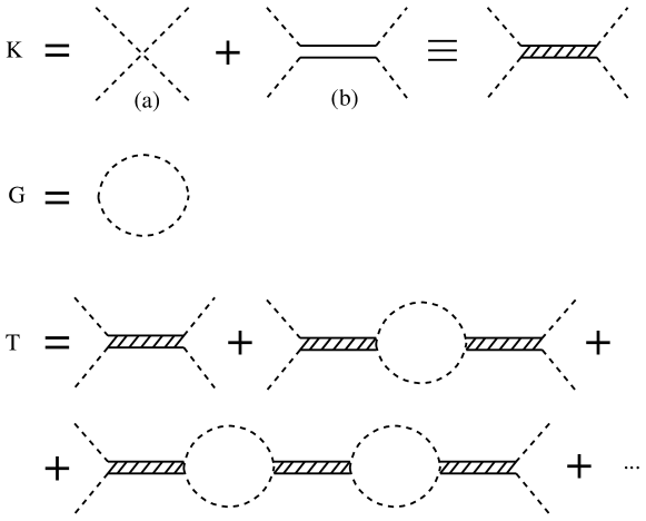
Figure 1: Diagrammatic representation of the matrices described in the text. (a) and (b) correspond to the amplitudes derived from the $\mathcal{O}(p^{2})$ and resonance chiral lagrangians respectively. The double solid line filled with short oblique dashes represents the effective scattering amplitude. Dashed lines are $\pi$, $K$ mesons.

In Fig. 1 we show a diagrammatic representation of the three matrices involved, $K(s)$, $G(s)$ and $T(s)$. The last one represents the resummation performed in eq. (3) with the unitarization procedure (N/D method).

The $d_{i}$ constants in eq. (4) are chosen to obey the low energy chiral constraints [32],

$$d_{K}=\frac{-2\ m_{\pi}^{2}}{m_{K}^{2}-m_{\pi}^{2}}\left(\log\frac{m_{\pi}^{2}}{\mu^{2}}+\frac{1}{2}\log\frac{m_{K}^{2}}{\mu^{2}}+\frac{1}{2}\right)$$

$$d_{\pi}=\frac{m_{K}^{2}}{m_{K}^{2}-m_{\pi}^{2}}\left(\log\frac{m_{\pi}^{2}}{\mu^{2}}+\frac{1}{2}\log\frac{m_{K}^{2}}{\mu^{2}}+\frac{1}{2}\right),$$ (5)

and they are obtained by matching the expressions of the form factors calculated in this approach with those of one loop $\chi PT$. In eq. (2) $\mu=770$ MeV and we have substituted index values $i=1,2$ by their actual meaning.

The regularization can also be carried out following a cut-off scheme. The loop functions with a cut-off in the three-momentum of the particles in the loop can be found in the appendix of ref. [26], and up to order $\frac{m_{i}}{q_{i}^{max}}$ they read

$$G^{C}_{i}(s)=\frac{1}{16\,\pi^{2}}\left[-2\,\log\frac{2\,q_{i}^{max}}{m_{i}}+\sigma_{i}(s)\,\log\frac{\sigma_{i}(s)+1}{\sigma_{i}(s)-1}\right],$$ (6)

where $q_{i}^{max}$ is the cut-off mentioned above. By comparing the expressions of the $G_{i}(s)$ functions in both schemes we can get the equivalent $q_{i}^{max}$ in order to keep the low energy chiral information of the $d_{i}$ constants, and therefore one can use equivalently any of the two procedures.

In Fig. 2 we show the $T_{22}$ matrix element vs invariant mass. To check how important is the inclusion of the $K\bar{K}$ channel we have performed the calculation in both coupled and decoupled cases. By decoupled case we mean turning off the $K\bar{K}\to\pi\pi$ interaction, what is easily done setting $K_{12}=0$ in eqs. (2) and (3). The conclusion is that kaon loops produce minimum changes in the results and therefore they can be ignored and we can work in a decoupled description in what concerns the $\pi\pi\to\pi\pi$ scattering amplitude. In the next sections we shall develop the model for scattering in nuclear matter. Although we formally work in the general scenario of the coupled channel approach, we perform our calculations in the decoupled case.

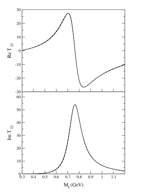
Figure 2: Real and imaginary parts of the $\pi\pi\to\pi\pi$ scattering amplitude ($T_{22}$ matrix element). The solid line curve is obtained with the coupled channel formalism including kaons, while the dashed curve is the result of the decoupled calculation.

It is interesting to establish connection with other approaches where tadpole terms are explicitly kept in the lagrangian. Indeed in [18] an explicit term appears in the lagrangian when the minimal coupling is used to introduce the gauge vector fields. A contact term,

$${\cal L}^{(ct)}=g_{\rho}^{2}\rho_{\mu}\rho^{\mu}\pi_{+}\pi_{-},$$ (7)

is obtained where $g_{\rho}$ is connected to our coupling via

$$g_{\rho}=-\frac{M_{\rho}G_{V}}{f^{2}}.$$ (8)

With this lagrangian one obtains a contribution to the $\rho$ selfenergy which is expressed in terms of the tadpole diagram in Fig. 3

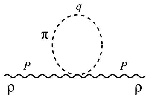
Figure 3: Tadpole diagram contributing to the $\rho$ meson selfenergy, coming from the $\rho\rho\pi\pi$ vertex. Wavy lines represent the $\rho$ meson in the gauge vector field formalism and dashed lines are pions.

and is given by

$$-it_{tad}=-i\Pi^{\mu\nu}\epsilon_{\mu}\epsilon_{\nu}=-2g_{\rho}^{2}\int\frac{d^{4}q}{(2\pi)^{4}}g^{\mu\nu}\epsilon_{\mu}\epsilon_{\nu}D_{0}(q),$$ (9)

where $D_{0}(q)$ is the free pion propagator. When we work with this formalism we simultaneously release the on shell condition in the $\rho\pi\pi$ vertex in the evaluation of the selfenergy diagram represented in Fig. 4 [26, 35].

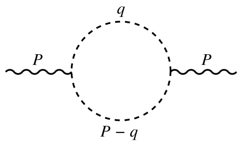
Figure 4: Two pion diagram contributing to the $\rho$ meson selfenergy.

Since we are interested in the $\rho$ at rest, we need only to evaluate the spatial components of $\Pi^{\mu\nu}$ and, thus, using the vector form of the $\rho\pi\pi$ coupling of [18],

$${\cal L}_{\rho\pi\pi}=ig_{\rho}\rho^{\mu}(\pi^{+}\partial_{\mu}\pi^{-}-\pi^{-}\partial_{\mu}\pi^{+}),$$ (10)

we obtain

$$\Pi^{ij}=ig_{\rho}^{2}\int\frac{d^{4}q}{(2\pi)^{4}}4q^{i}q^{j}D_{0}(P-q)D_{0}(q)-ig_{\rho}^{2}\int\frac{d^{4}q}{(2\pi)^{4}}2g^{ij}D_{0}(q).$$ (11)

By using dimensional regularization it is easy to prove that

$$\int\frac{d^{4}q}{(2\pi)^{4}}\frac{4q^{\mu}q^{\nu}}{(q^{2}+s+i\epsilon)^{2}}=\int\frac{d^{4}q}{(2\pi)^{4}}\frac{2g^{\mu\nu}}{q^{2}+s+i\epsilon}.$$ (12)

Then eq. (11) can be written as

$$\Pi^{ij}=ig_{\rho}^{2}\int\frac{d^{4}q}{(2\pi)^{4}}4q^{i}q^{j}[D_{0}(P-q)D_{0}(q)-D_{0}(q)^{2}]$$

$$=ig_{\rho}^{2}\frac{4}{3}\delta^{ij}\int\frac{d^{3}q}{(2\pi)^{3}}\int\frac{dq^{0}}{2\pi}\vec{q}\,^{2}[D_{0}(P-q)D_{0}(q)-D_{0}(q)^{2}]$$

$$=ig_{\rho}^{2}\frac{4}{3}\delta^{ij}\int\frac{d^{3}q}{(2\pi)^{3}}\int\frac{dq^{0}}{2\pi}\vec{q}\,^{2}[D_{0}(P-q)D_{0}(q)-\frac{\partial}{\partial m_{\pi}^{2}}D_{0}(q)].$$ (13)

The $q^{0}$ integration is now easy to perform and we obtain

$$\Pi^{ij}=g_{\rho}^{2}\frac{4}{3}\delta^{ij}\int\frac{d^{3}q}{(2\pi)^{3}}\bigg{[}\frac{\vec{q}\,^{2}}{\omega(q)}\frac{1}{(P^{0})^{2}-4\omega(q)^{2}+i\epsilon}+\frac{\vec{q}\,^{2}}{\omega(q)}\frac{1}{4\omega(q)^{2}}\bigg{]},$$ (14)

where $\omega(q)^{2}=m_{\pi}^{2}+\vec{q}\,^{2}$.

Now, if we separate in the first term of eq. (14) the on shell and off shell contribution of the factor $\vec{q}\,^{2}$ in the numerator, which comes from the $\rho\pi\pi$ vertices, we have $\vec{q}\,^{2}=\vec{q}\,^{2}_{on}+\vec{q}\,^{2}_{off}$ with $\vec{q}\,^{2}_{on}=(\frac{P^{0}}{2})^{2}-m_{\pi}^{2}$. Since we have $(P^{0})^{2}-4\,\omega(q)^{2}=-4(\vec{q}\,^{2}-\vec{q}\,^{2}_{on})$ then the contribution of the tadpole plus the off shell piece of the two pion loop diagram is given by

$$\tilde{\Pi}^{ij}=-g_{\rho}^{2}\frac{m_{\pi}^{2}}{3}\delta^{ij}\int\frac{d^{3}q}{(2\pi)^{3}}\frac{1}{\omega(q)^{3}}$$ (15)

which is a logarithmically divergent piece independent of $P^{0}$ and hence can be absorbed in a renormalization of the $\rho$ bare mass.

The former exercise proves that the formalism keeping tadpoles and full off shell dependence of the $\rho\pi\pi$ vertex is equivalent to the one we have showed above where only the on shell part of the $\rho\pi\pi$ vertex is kept and no tadpole is included.

In the medium, however, the pion propagator in the tadpole term will change. Hence, in order to stick to the gauge invariance of the vector field formalism we shall keep this tadpole term [12, 17, 18].

3 $(I,J)=(1,1)$ $\pi\pi$ scattering in the nuclear medium

We now address the calculation in the presence of nuclear matter. As already mentioned, the $\rho$ meson couples to intermediate two-meson states. Medium corrections will be incorporated in the selfenergies of the mesons involved and the related vertex corrections as well as from direct coupling to the hadrons in particle-hole ($p-h$) and delta-hole ($\Delta-h$) excitations. We briefly discuss below the input used for the pion selfenergy.

3.1 Pion selfenergy in dense nuclear matter

The pion selfenergy in the nuclear medium originates from $p-h$ and $\Delta-h$ excitations, corresponding to diagrams in Fig. 5. We describe the selfenergy as usual in terms of the ordinary Lindhard function, which automatically accounts for forward and backward propagating bubbles, hence including both diagrams of Fig. 5. Short range correlations are also considered with the Landau-Migdal parameter $g^{\prime}$ set to $0.7$. The final expression reads

$$\Pi_{\pi}(q,\rho)=f(\vec{q}\,^{2})^{2}\vec{q}\,^{2}\frac{C\,U(q,\rho)}{1-C\,g^{\prime}U(q,\rho)},$$ (16)

where here $q$ is the four-momentum of the pion, $\rho$ stands for the nuclear density and $C=(\frac{D+F}{2f})^{2}$. The Lindhard function, $U=U_{N}+U_{\Delta}$, contains both $p-h$ and $\Delta-h$ contributions. Formulae for $U_{N}$ and $U_{\Delta}$ with the normalization required here can be found in the appendix of ref. [37]. We use a monopole form factor $f(\vec{q}\,^{2})=\frac{\Lambda^{2}}{\Lambda^{2}+\vec{q}\,^{2}}$ for the $\pi NN$ and $\pi N\Delta$ vertices with the cut-off parameter set to $\Lambda=1$ GeV. In the case of the $\pi N\Delta$ vertex we also include a recoil factor $M_{N}/\sqrt{s_{\Delta}}$ to account for the fact that the momentum $\vec{q}$ in the $\pi N\Delta$ vertex should be in $\Delta$ CM frame. We will check the sensitivity of our results to variations of both the $\Lambda$ and $g^{\prime}$ parameters.

Figure 5: Direct and crossed $p-h$, $\Delta-h$ excitation terms giving rise to the pion selfenergy in the nuclear medium, expressed in terms of the Lindhard function as described in the text.

3.2 Gauge invariant contact terms

In our microscopic model of $\pi\pi$ scattering in nuclear matter all graphs in Fig. 6 are considered. In addition to the single $p-h$ excitation (diagram 6a) we have to account for the medium modifications of the $\rho$-meson-meson vertex via the $\rho$-meson-baryon contact term, as requested by the gauge invariance of the

Figure 6: Medium correction graphs: single solid lines are reserved for particle-hole excitations.

theory [12, 16, 17]. Hence we need to evaluate also the diagrams 6b to 6d. This contact term can be constructed in a similar way as it was done in [36] for the $\phi$ decay in the nuclear medium. Let us study the set of diagrams depicted in Fig. 7, for the case of an incoming $\pi^{+}$. The amplitude corresponding to the graph 7a in the gauge vector formulation of the $\rho$ is readily

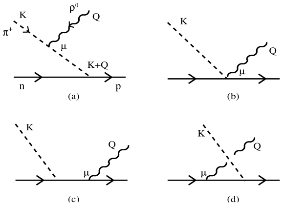
Figure 7: Gauge invariant set of diagrams used to calculate the $\rho$-meson-baryon contact term as explained in the text. The wavy lines represent here the vector meson, the dashed ones pions and the solid lines are reserved for nucleons.

evaluated and its contribution is

$$-it=i\frac{M_{\rho}G_{V}}{f^{2}}\epsilon_{\mu}(Q+2K)^{\mu}\frac{i}{(Q+K)^{2}-m_{\pi}^{2}}\sqrt{2}(\frac{D+F}{2f})\vec{\sigma}(\vec{K}+\vec{Q}),$$ (17)

where $K$ and $Q$ are four-momenta of the pion and the $\rho$ meson respectively, $\vec{\sigma}$ is the spin-$\frac{1}{2}$ operator and $\epsilon_{\mu}$ is the polarization vector of the $\rho$ meson. The contact term, represented by Fig. 7b, must have the structure

$$-it_{cont}=\epsilon_{\mu}B^{\mu},$$ (18)

and gauge invariance requires that if we replace $\epsilon_{\mu}$ by $Q_{\mu}$ then the sum of all the terms in Fig. 7 vanishes. To find out the strength of the coupling we shall take the limit $\vec{K}\to\vec{0}$ because in that case diagrams 7c and 7d give a null contribution and we have to consider only the sum of the first two so far commented. Then we find the following system of equations:

$$B^{0}=0$$

$$-\frac{M_{\rho}G_{V}}{f^{2}}\sqrt{2}(\frac{D+F}{2f})\vec{\sigma}\vec{Q}-\vec{B}\vec{Q}=0.$$ (19)

After solving for $B^{\mu}$, the amplitude corresponding to diagram 7b is

$$-it_{cont}=\frac{M_{\rho}G_{V}}{f^{2}}\sqrt{2}(\frac{D+F}{2f})\vec{\sigma}\vec{\epsilon},$$ (20)

and with this information the whole set of diagrams in Fig. 6 can be evaluated. Note that because of the $\rho$ coupling to the pions, eq. (20) has a minus sign for an incoming $\pi^{-}$.

3.3 Technical implementation of vertex corrections

In the previous section we have commented that gauge invariance requires the presence of the $\rho$-meson-baryon contact term, which results in the need of including diagrams b, c and d in Fig. 6. Now we pay attention on how these vertex corrections can be incorporated in the unitary treatment of the $T$ matrix described in section 2. To this end let us

Figure 8: Momentum labels for the in-medium correction diagrams. $D_{0}$ indicates a pion propagator and $\Pi$ refers to the pion selfenergy due to $p-h$ excitation.

consider in detail the set of diagrams 6a, b and c . The momentum labelling is shown in Fig. 8 for the first diagram (the pion in the upper line will have four-momentum $q$ and the one in the lower line ($P-q$)). The amplitudes originating from these graphs in the gauge vector formulation of the $\rho$ are evaluated using Feynman rules and the results are

$$A_{(a)} = \int{\frac{d^{4}q}{(2\pi)^{4}}V_{\rho\pi\pi}(q)^{2}iD_{0}(q)iD_{0}(P-q)\bigg{[}-i(\frac{D+F}{2f})^{2}\vec{q}\,^{2}U(q,\rho)\bigg{]}iD_{0}(q)}$$

$$A_{(b)} = \int{\frac{d^{4}q}{(2\pi)^{4}}V_{\rho\pi\pi}(q)^{2}\frac{1}{2}\bigg{[}(\frac{D+F}{2f})^{2}U(q,\rho)\bigg{]}iD_{0}(q)iD_{0}(P-q)}$$

$$A_{(c)} = A_{(b)}$$ (21)

where $V_{\rho\pi\pi}$ stands for the $\rho\pi\pi$ vertex,

$$V_{\rho\pi\pi}=-i\frac{M_{\rho}G_{V}}{f^{2}}2\vec{\epsilon}\vec{q}$$ (22)

and $D_{0}(q)$ is the bare propagator of a pion with four-momentum $q$. The subindices (a), (b) and (c) refer to each diagram in Fig. 6. In $A_{(a)}$ we have explicitly substituted the expression of the pion selfenergy due to a $p-h$ or $\Delta-h$ excitation, which would read

$$-i\Pi(q,\rho)=-i(\frac{D+F}{2f})^{2}\vec{q}\,^{2}U(q,\rho).$$ (23)

It is obvious that the sum of all three diagrams,

$$A_{(a)}+A_{(b)}+A_{(c)}={}$$ (24)

$${}\int{\frac{d^{4}q}{(2\pi)^{4}}V_{\rho\pi\pi}(q)^{2}iD_{0}(q)iD_{0}(P-q)\bigg{[}(\frac{D+F}{2f})^{2}U(q,\rho)\bigg{]}(\vec{q}\,^{2}D_{0}(q)+1)},$$

can be cast in the form of $A_{(a)}$ if we substitute the $\vec{q}\,^{2}$ appearing in eq. (23) by

$$\vec{q}\,^{2}\to\vec{q}\,^{2}+D_{0}^{-1}(q).$$ (25)

We still have to consider the last diagram in Fig. 6, 6d. It is easy to find, in the same way as before, that the amplitude can be cast in the structure of $A_{(a)}$ making the substitution

$$\vec{q}\,^{2}\to\frac{3}{4}\frac{D_{0}^{-2}(q)}{\vec{q}\,^{2}}$$ (26)

in eq. (23). Hence, we find that vertex corrections can be automatically introduced in the gauge vector formulation of the problem by performing the following substitution

$$\vec{q}\,^{2}\to H_{vc}(q)\equiv\vec{q}\,^{2}+D_{0}^{-1}(q)+\frac{3}{4}\frac{D_{0}^{-2}(q)}{\vec{q}\,^{2}}$$ (27)

in the pion selfenergy described in eq. (16), hence working with a kind of an ’extended’ pion selfenergy which takes care of the medium modifications of the $\rho\pi\pi$ vertex, namely

$$-i\Pi^{ext}(q,\rho)=-if(\vec{q}\,^{2})^{2}H_{vc}(q)\frac{(\frac{D+F}{2f})^{2}U(q,\rho)}{1-(\frac{D+F}{2f})^{2}g^{\prime}U(q,\rho)}.$$ (28)

The calculation of the $\pi\pi$ scattering matrix in the medium follows the calculation of the $G(s)$ function for pions. As it was mentioned in section 2 we keep full off shell dependence of the $\rho\pi\pi$ vertex. The medium effects are introduced by a subtraction of the $\rho$ meson selfenergy due to pion loops in free space from the same quantity calculated in nuclear matter. The following substitution is performed in eq. (4):

$$G(s)\to G(s)+\frac{1}{\vec{q}\,^{2}_{on}}[I_{med}(s)-I_{free}(s)],$$ (29)

where

$$I_{med}(s) = i\int\frac{d^{4}q}{(2\pi)^{4}}\vec{q}\,^{2}D(q)D(P-q)$$

$$I_{free}(s) = i\int\frac{d^{4}q}{(2\pi)^{4}}\vec{q}\,^{2}D_{0}(q)D_{0}(P-q)$$ (30)

and $D(q)$ is the in-medium pion propagator,

$$D(q)=\frac{1}{q^{2}-m_{\pi}^{2}-\Pi_{\pi}(q,\rho)}.$$ (31)

To include the vertex corrections discussed above, the pion selfenergy $\Pi_{\pi}(q,\rho)$ in the latter equation must be replaced by the one in eq. (28).

Each of the integrals in eq. (29) are quadratically divergent. The subtraction $I_{med}-I_{free}$ cancels these quadratic divergences and we are left with a logarithmic divergence which in principle has to be regularized with a cut off in the pion loop momentum. However, notice that $D(q)D(q)-D_{0}(q)D_{0}(q)$ is proportional to $\Pi^{ext}(q,\rho)$. Therefore, since all the pieces that enter $\Pi^{ext}(q,\rho)$ are multiplied by a squared form factor $f(\vec{q}\,^{2})^{2}$ the subtraction is convergent.

3.4 Rho meson propagator from the T matrix

For the sake of simplicity, and having in mind the results of section 2, we turn off the interaction between $\pi\pi$ and $K\bar{K}$ systems and work in a decoupled channel approach ($K_{12}=0$ in eqs. (2) and (3)). Then the $\pi\pi\to\pi\pi$ $T$ matrix element takes the simple form

$$T_{22}=\frac{1}{1+K_{22}G}K_{22}$$ (32)

Let us first assume that $\frac{2G_{V}^{2}}{f^{2}}=1$, as it is indeed the case if VMD holds exactly. Then the $K_{22}$ matrix element reads

$$K_{22}=-\frac{2}{3}\frac{p_{\pi}^{2}M_{\rho}^{2}}{f^{2}}\frac{1}{s-M_{\rho}^{2}},$$ (33)

where one can identify the p-wave structure of the $\pi\pi\to\pi\pi$ scattering amplitude mediated by the exchange of a $\rho$ meson. Hence the factor $(1+K_{22}G)^{-1}$ in eq. (32) is accounting for a selfenergy of the $\rho$ meson arising from the coupling with $\pi\pi$ pairs (to switch on the presence of the nuclear medium one has just to perform the substitution of eq. (29) as described in section 3 with the modified pion selfenergy of eq. (28)). We can therefore write eq. (32) as

$$T_{22} = -\frac{2}{3}\frac{p_{\pi}^{2}M_{\rho}^{2}}{f^{2}}\frac{1}{s-M_{\rho}^{2}-\Pi_{\rho}^{\pi-loop}}$$

$$\Pi_{\rho}^{\pi-loop} = -K_{22}G(s-M_{\rho}^{2})\,=\,\frac{2}{3}\frac{p_{\pi}^{2}M_{\rho}^{2}}{f^{2}}G,$$ (34)

where $\Pi_{\rho}^{\pi-loop}$ is the selfenergy commented above.

Now we consider the case $\frac{2G_{V}^{2}}{f^{2}}\neq 1$. Let $a\equiv\frac{2G_{V}^{2}}{f^{2}}$ and proceed as above. The $K_{22}$ matrix element can be easily cast in the form

$$K_{22}=-\frac{2}{3}\frac{p_{\pi}^{2}M_{\rho}^{2}}{f^{2}}B(s)\frac{1}{s-M_{\rho}^{2}}$$ (35)

where $B(s)\equiv 1+(a-1)\frac{s}{M_{\rho}^{2}}$. Eq. (35) reduces to eq. (33) if $a=1$, because in that case $B=1$ independently of $s$. For the values of $G_{V}$ and $f$ of [32] we find that $a$ takes the value $\approx 0.7$. For instance, at $s=M_{\rho}^{2}$ we have $B(M_{\rho}^{2})\approx 0.7$, therefore a 30 % of deviation from VMD is introduced. The $T$ matrix element for $\pi\pi\to\pi\pi$ scattering now reads

$$T_{22} = -\frac{2}{3}\frac{p_{\pi}^{2}M_{\rho}^{2}}{f^{2}}B(s)\frac{1}{s-M_{\rho}^{2}-\Pi_{\rho}^{\pi-loop}}=-\tilde{g}^{2}\frac{4}{3}p_{\pi}^{2}D_{\rho}(s)$$

$$\Pi_{\rho}^{\pi-loop} = \frac{2}{3}\frac{p_{\pi}^{2}M_{\rho}^{2}}{f^{2}}B(s)G\,=\,\tilde{g}^{2}\frac{4}{3}p_{\pi}^{2}G,$$ (36)

where $\tilde{g}^{2}=\frac{1}{2}\frac{M_{\rho}^{2}}{f^{2}}B(s)$ defines a coupling which will replace $g_{\rho}^{2}$ in our formulae, and $D_{\rho}$ is the $\rho$ meson propagator.

In the following sections we shall discuss about the tadpole term in the nuclear medium as well as new contributions due to the direct coupling of the $\rho$ meson to the baryonic lines in particle and delta-hole excitations. These new contributions will manifest as additional pieces to the whole $\rho$ meson selfenergy $\Pi$. The way of introducing these new pieces in the $T$ matrix and the $\rho$ propagator follows the same scheme as it has been done with the contribution from two pion loop selfenergy plus its vertex corrections, $\Pi_{\rho}^{\pi-loop}$.

3.5 Tadpole term in nuclear matter

We have seen that keeping the full off shell dependence of the $\rho\pi\pi$ vertex and explicitly considering the free tadpole term in the calculation of the $\rho$ meson selfenergy is equivalent to calculating with the on shell part of the $\rho\pi\pi$ vertex and describing the pion loop contributions with the $G(s)$ functions defined in section 2. This freedom allows us to include the tadpole diagram in nuclear matter by performing a subtraction between the selfenergies corresponding to the tadpole term in the medium and in free space. In the gauge vector field approach one has

$$-i\Pi_{\mu\nu}^{tad}=-2g_{\rho}^{2}g_{\mu\nu}\int\frac{d^{4}q}{(2\pi)^{4}}D_{0}(q).$$ (37)

The $\rho$ selfenergy, $\Pi$, which appears in the $\rho$ propagator in the former section can be related to $\Pi_{\mu\nu}$ by

$$\Pi_{\mu\nu}=\bigg{\{}-g_{\mu\nu}+\frac{P^{\mu}P^{\nu}}{M_{\rho}^{2}}\bigg{\}}\Pi,$$ (38)

and restricting ourselves to the space components of $\mu$, $\nu$ we have for the tadpole piece

$$\Pi^{tad}=2ig_{\rho}^{2}\int\frac{d^{4}q}{(2\pi)^{4}}D_{0}(q).$$ (39)

We define the subtracted in medium tadpole contribution to the $\rho$ meson selfenergy as

$$\tilde{\Pi}^{tad}(\rho)=2ig_{\rho}^{2}\int\frac{d^{4}q}{(2\pi)^{4}}[D(q)-D_{0}(q)].$$ (40)

Given the analytical structure of $D(q)$ and $D_{0}(q)$ by performing a Wick rotation one can see that $\tilde{\Pi}^{tad}$ is real, and eq. (40) can be rewritten as

$$\tilde{\Pi}^{tad}(\rho)=-2g_{\rho}^{2}\int\frac{d^{4}q}{(2\pi)^{4}}[ImD(q)-ImD_{0}(q)].$$ (41)

Taking into account that both $D_{0}(q)$ and $D(q)$ are even functions of $q^{0}$, the integration in $q^{0}$ can be replaced by twice the integration from $0$ to $\infty$. This integration can be performed analytically for the second term of eq. (41) and we obtain

$$\tilde{\Pi}^{tad}(\rho)=-4g_{\rho}^{2}\int\frac{d^{3}q}{(2\pi)^{3}}\bigg{[}\int_{0}^{\infty}\frac{dq^{0}}{2\pi}ImD(q)+\frac{1}{4\omega(q)}\bigg{]}.$$ (42)

Eq. (42) is free from quadratic divergences. Actually the form factors present in the pion selfenergy make it convergent and a cut off in the pion loop momentum is not required.

3.6 Other medium corrections

As it has been discussed in subsections 3.2 and 3.3, gauge invariance provides us with $\rho\pi NN$, $\rho\pi N\Delta$ contact vertices which give rise to the diagrams depicted in Fig. 6. In addition to those there are other medium corrections that arise within the gauge vector field formalism and generate interactions via the minimal coupling scheme (the former contact vertices can also be obtained in this way). Let us summarize the interaction lagrangians of ref. [18] involving $\rho\pi\pi$, $\rho\rho\pi\pi$, $\pi NN$, $\pi N\Delta$, $\rho NN$, $\rho\pi NN$, $\rho\Delta\Delta$ and $\rho\pi N\Delta$ vertices:

$${\cal L}_{\pi\rho} = {1\over 2}ig_{\rho}\rho_{\mu}(T_{3}\vec{\phi}\partial^{\mu}\vec{\phi}+\partial^{\mu}\vec{\phi}T_{3}\vec{\phi})-{1\over 2}g_{\rho}^{2}\rho_{\mu}\rho^{\mu}T_{3}\vec{\phi}T_{3}\vec{\phi}$$

$${\cal L}_{\pi NN} = {f_{N}\over{m_{\pi}}}\,\bar{\psi}\gamma^{5}\gamma^{\mu}\vec{\tau}\psi\partial_{\mu}\vec{\phi}$$

$${\cal L}_{\pi N\Delta} = -{f_{\Delta}\over{m_{\pi}}}\bar{\psi}\vec{T}^{{\dagger}}\psi_{\mu}\partial^{\mu}\vec{\phi}\quad+\quad\mbox{h.c.}$$

$${\cal L}_{\rho NN} = -{g_{\rho}\over 2}\bar{\psi}\rho\!\!\!/\tau_{3}\psi$$

$${\cal L}_{\rho\pi NN} = ig_{\rho}{f_{N}\over{m_{\pi}}}\bar{\psi}\gamma^{5}\rho\!\!\!/\vec{\tau}\psi T_{3}\vec{\phi}$$

$${\cal L}_{\rho\Delta\Delta} = g_{\rho}\bar{\psi}_{\mu}\rho\!\!\!/T_{3}^{({3\over 2})}\psi^{\mu}-{g_{\rho}\over 3}\bar{\psi}_{\mu}(\gamma^{\mu}\rho_{\nu}+\gamma_{\nu}\rho^{\mu})T_{3}^{({3\over 2})}\psi^{\nu}+{g_{\rho}\over 3}\bar{\psi}_{\mu}\gamma^{\mu}\rho\!\!\!/T_{3}^{({3\over 2})}\gamma_{\nu}\psi^{\nu}$$

$${\cal L}_{\rho\pi N\Delta} = -ig_{\rho}{f_{\Delta}\over{m_{\pi}}}\bar{\psi}\vec{T}^{{\dagger}}\psi_{\mu}\rho^{\mu}T_{3}\vec{\phi}\quad+\quad\mbox{h.c.}$$ (43)

From the list above, lagrangians generating direct couplings of a $\rho$ meson to either a nucleon or a delta were not considered in subsection 3.2. As we will discuss below, these terms give rise to a set of diagrams correcting both the $\rho$ meson selfenergy from two pion loop and tadpole terms.

Before proceeding with the discussion of the new contributions, it is interesting to comment on the relative sign of the $\rho\pi\pi$ coupling constant in the language of chiral lagrangians and in the gauge vector field formalism. From eq. (3.6), the $\rho\pi\pi$ vertex takes the form

$$-it_{\rho\pi\pi}=-ig_{\rho}\epsilon_{\mu}(p-p^{\prime})^{\mu},$$ (44)

with the momentum labels corresponding to Fig. 9.

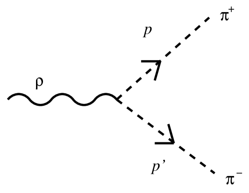
Figure 9: $\rho\pi\pi$ vertex. Lines as in Fig. 7

However, in our model we would write

$$-it_{\rho\pi\pi}=i\frac{M_{\rho}G_{V}}{f^{2}}\epsilon_{\mu}(p-p^{\prime})^{\mu},$$ (45)

and this establishes the correspondence

$$g_{\rho}=-\frac{M_{\rho}G_{V}}{f^{2}}$$ (46)

to connect both schemes. As an example, following the lagrangians listed above, eq. (20) reads

$$-it_{cont}=-g_{\rho}{f_{N}\over{m_{\pi}}}\sqrt{2}\vec{\sigma}\vec{\epsilon},$$ (47)

which reconfirms the relationship of eq. (46).

3.6.1 Extra two-pion loop correction to the $\rho$ selfenergy

The first additional medium correction that we consider here is the one shown in Fig. 10, with the $\rho$ meson attached to a particle line.

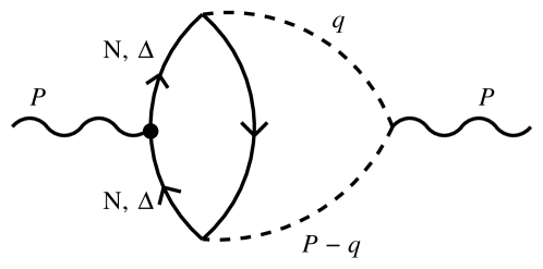
Figure 10: Vertex correction involving $\rho NN$, $\rho\Delta\Delta$ vertices.

As we shall show below, this contribution can also be cast in the form of a vertex correction to be introduced in the ’extended’ pion selfenergy of eq. (28). Following the Feynman rules for the vertices involved (after a non-relativistic reduction) the $\rho$ meson selfenergy contribution from this diagram ($N-h$ case, $P^{0}=\sqrt{s}$) reads

$$-i\Pi_{1,\rho NN}^{ij} = \delta^{ij}g_{\rho}^{2}\frac{4}{3}\frac{1}{M_{N}\sqrt{s}}\bigg{(}{f_{N}\over{m_{\pi}}}\bigg{)}^{2}\int\frac{d^{4}q}{(2\pi)^{4}}(\vec{q}\,^{2})^{2}D_{0}(q)D_{0}(P-q){}$$ (48)

$${}\frac{1}{2}[\bar{U}_{N}(q^{0}-\sqrt{s},\vec{q})-\bar{U}_{N}(q^{0},\vec{q})+\bar{U}_{N}(-q^{0},\vec{q})-\bar{U}_{N}(-q^{0}+\sqrt{s},\vec{q})],$$

where the $\bar{U}_{N}$ functions account for the direct contribution of a nucleon-hole excitation (Fig. 5, left) and sum over spin but not over isospin. They satisfy the relation

$$2\,[\bar{U}_{N}(q^{0},\vec{q})+\bar{U}_{N}(-q^{0},\vec{q})]=U_{N}(q^{0},\vec{q}).$$ (49)

In the case of a $\rho$ meson coupling to a $\Delta$ line one obtains a similar expression, with different spin/isospin factors and a scaling factor to the $\pi\pi N$ coupling, if a constant $\Delta$ width is considered. The reason is that in the nucleon case one is allowed to express the product of two particle propagators as the difference of such propagators times $s^{-\frac{1}{2}}$. Then the resulting expression of $\Pi^{ij}$ can be written in terms of the $\bar{U}_{N}$ functions. However, keeping the $\Delta$ width is important and, hence, we shall keep its energy dependence and use another approximation to the integral of the two $\Delta$ and one hole propagators appearing in the expression of $\Pi^{ij}$. The calculation is the done by making a Fermi average over the two $\Delta$ propagators.

Given the structure of this correction it is convenient to incorporate it by means of corrections to the pion selfenergy in the two pion propagators of eq. (3.3). This is accomplished by means of the substitution

$$\vec{q}\,^{2}U(q^{0},\vec{q})\to\vec{q}\,^{2}U(q^{0},\vec{q})+(\alpha_{N}+\alpha_{\Delta})D_{0}^{-1}(q^{0},\vec{q}),$$ (50)

with

$$\alpha_{N} = \frac{\vec{q}\,^{2}}{2M_{N}\sqrt{s}}[\bar{U}_{N}(q^{0}-\sqrt{s},\vec{q})-\bar{U}_{N}(q^{0},\vec{q})+\bar{U}_{N}(-q^{0},\vec{q})-\bar{U}_{N}(-q^{0}+\sqrt{s},\vec{q})]$$

$$\alpha_{\Delta} = \frac{\vec{q}\,^{2}}{2M_{\Delta}}\frac{10}{9}\bigg{(}\frac{f_{\Delta}}{f_{N}}\bigg{)}^{2}\frac{\rho}{2}\bigg{\{}G_{\Delta}(q^{0}-\sqrt{s},\vec{q})G_{\Delta}(q^{0},\vec{q})+{}$$ (51)

$${}G_{\Delta}(-q^{0},\vec{q})G_{\Delta}(-q^{0}+\sqrt{s},\vec{q})\bigg{\}}$$

and

$$G_{\Delta}(q^{0},\vec{q})=\frac{1}{\sqrt{s_{\Delta}}-M_{\Delta}+\frac{i}{2}\Gamma_{\Delta}(s_{\Delta})}$$

$$s_{\Delta}=M_{N}^{2}+(q^{0})^{2}-\vec{q}\,^{2}+2q^{0}\sqrt{M_{N}^{2}+\frac{3}{5}k_{F}^{2}}.$$ (52)

Expressions for the energy dependent $\Delta$ width can be found in [37].The substitution of eq. (50) already accounts for the two possible time orderings in Fig. 10: incoming $\rho$ meson coupled to the baryon loop, outgoing $\rho$ meson closing the two pion loop, and vice versa. Notice that in eq. (3.6.1) we have not used the common non-relativistic approximation of $G_{\Delta}^{-1}$ since it is not appropriate for this case because high momenta contribute to the loop integrals. The same argument is of application for the corrections discussed in the next section.

3.6.2 Tadpole like corrections

We study now a set of diagrams containing $\rho NN$, $\rho\Delta\Delta$ vertices which are generated from those in the former section by contracting one pion line, in analogy to the way the vertex corrections in Figs. 6b, 6c where generated from Fig. 6a. These terms are related to the diagrams labelled as $\rho\rho\pi\pi$ vertex correction in [18]. The diagrams are shown in Fig. 11,

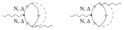
Figure 11: Additional medium corrections. The pion line represent either a $\pi^{+}$ or a $\pi^{-}$. The partners with the outgoing $\rho$ attached to the nucleon (or $\Delta$) line are not displayed.

although the set includes also the partners with an outgoing $\rho$ meson attached to a nucleon (or $\Delta$) line.

The selfenergy corresponding to the diagrams in Fig. 11 and their partners for the nucleon case reads

$$-i\Pi_{2,\rho NN}^{ij}=\frac{4}{3}\frac{g_{\rho}^{2}}{M\sqrt{s}}\bigg{(}{f_{N}\over{m_{\pi}}}\bigg{)}^{2}\delta^{ij}\int\frac{d^{4}q}{(2\pi)^{4}}\vec{q}\,^{2}D_{0}(q)[\bar{U}_{N}(q^{0}-\sqrt{s},\vec{q})-\bar{U}_{N}(q^{0}+\sqrt{s},\vec{q})],$$ (53)

where the factor four indicates that the contributions of protons or neutrons over the Fermi sea are identical, and the same happens for the diagrams with the incoming and outgoing $\rho$ mesons interchanged.

For the case of the $\Delta$ isobar, the number of diagrams involved are twice the number for the nucleon case, since now the $\Delta$ can be excited to its four charge states. As it happened in the previous subsection the result cannot be expressed in terms of modified Lindhard functions. Instead, we use the same approximation as before for the integration of the fermionic loop and we get

$$-i\Pi_{2,\rho\Delta\Delta}^{ij} = \frac{4}{3}\frac{g_{\rho}^{2}}{M_{\Delta}}\frac{10}{9}\bigg{(}{f_{N}\over{m_{\pi}}}\bigg{)}^{2}\bigg{(}{f_{\Delta}\over f_{N}}\bigg{)}^{2}\delta^{ij}\int\frac{d^{4}q}{(2\pi)^{4}}\vec{q}\,^{2}D_{0}(q){}$$ (54)

$${}\frac{\rho}{2}\bigg{\{}G_{\Delta}(q^{0}+\sqrt{s},\vec{q})G_{\Delta}(q^{0},\vec{q})+G_{\Delta}(q^{0},\vec{q})G_{\Delta}(q^{0}-\sqrt{s},\vec{q})\bigg{\}}.$$

3.6.3 Hartree like nucleon tadpole term

In ref. [18] we find no other medium corrections to the $\rho\pi\pi$ and $\rho\rho\pi\pi$ vertex functions, since the $\rho$ coupling to baryons is treated in a non-relativistic approach up to order $(1/M_{N})^{0}$. At next order an additional four point $\rho\rho NN$ vertex enters the calculation. This can be seen in ref. [17] where this vertex is generated by minimal substitution in a non-relativistic treatment of the $\rho NN$ lagrangian.

The same result can be obtained by calculating the $\rho N\to\rho N$ amplitude in the relativistic theory and then performing the non-relativistic reduction up to order $M_{N}^{-1}$. This is schematically shown in Fig. 12. In this non-relativistic reduction we obtain the nucleon direct and crossed pole terms of Fig. 12b with non-relativistic propagators and vertices, plus a contact term of order $M_{N}^{-1}$.

Figure 12: Diagrammatic representation of the non-relativistic reduction of the $\rho N\to\rho N$ amplitude.

If the nucleon lines of this last diagram are closed one obtains a nucleon tadpole diagram (Fig. 13b) which contributes as an additional linear-in-density piece of the $\rho$ meson selfenergy [17].

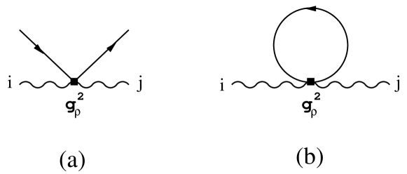
Figure 13: (a) $\rho\rho NN$ vertex. (b) Nucleon tadpole term.

The Feynman rule for the $\rho\rho NN$ vertex (Fig. 13a) can be derived from the $\rho N\to\rho N$ amplitude and it reads

$$-it_{\rho\rho NN}^{ij}=-ig_{\rho}^{2}\frac{1}{4}\frac{1}{M_{N}}\delta^{ij},$$ (55)

and the nucleon tadpole term is easily evaluated,

$$-i\Pi_{\rho\rho NN}^{ij}=-\delta^{ij}g_{\rho}^{2}\frac{1}{M_{N}}\int\frac{d^{4}p}{(2\pi)^{4}}\frac{n(\vec{p})}{p^{0}-\mathcal{E}_{N}(\vec{p})-i\epsilon}$$

$$=-i\delta^{ij}g_{\rho}^{2}\frac{1}{M_{N}}\int\frac{d^{3}p}{(2\pi)^{3}}n(\vec{p})=-i\delta^{ij}g_{\rho}^{2}\frac{1}{4}\frac{1}{M_{N}}\rho.$$ (56)

The result is an energy independent function proportional to the nuclear matter density. Its inclusion as a selfenergy term in the $\rho$ meson propagator follows the same procedure as already discussed for other contributions.

Finally, some other medium corrections involving $\rho BB$, $\rho\pi BB^{\prime}$ and $\rho\rho BB$ vertices can be considered but they either vanish or are very small and we discuss them briefly in the appendices.

4 $N^{*}(1520)-h$ contribution to the $\rho$ meson selfenergy

Next we intend to modify our formalism so that the $\rho$ meson is able to excite baryonic resonances via a $\rho NN^{*}$ coupling. From now on we will restrict the discussion to the case of $N^{*}(1520)$ $I(J^{P})=\frac{1}{2}(\frac{3}{2}^{-})$, although the same arguments considered here may be used to introduce other resonances with different quantum numbers .

The correction under discussion (excitation of a $N^{*}-h$ pair) will manifest as an extra selfenergy term in the $\rho$ propagator. The basic vertex involved in this effect is shown in Fig. 14a, and the lagrangian describing the interaction reads [38]

$$\mathcal{L}_{N^{*}N\rho}=-g_{N^{*}N\rho}\bar{\Psi}_{N}S_{i}\vec{\phi_{i}}\vec{\tau}\Psi_{N^{*}}+h.c.,$$ (57)

where $\Psi_{N}$, $\Psi_{N^{*}}$, $\phi_{i}$ are the $N$, $N^{*}(1520)$, $\rho$ fields, $S_{i}$ is the $\frac{1}{2}\to\frac{3}{2}$ spin transition operator, $\vec{\tau}$ is the isospin-$\frac{1}{2}$ operator and $g_{N^{*}N\rho}$ stands for the $\rho NN^{*}$ coupling constant that we take from [38] to be $g_{N^{*}N\rho}=7.73/\sqrt{3}$.

Figure 14: (a) $\rho NN^{*}$ vertex. (b) $N^{*}-h$ bubble contributing to the selfenergy of the $\rho$ meson.

Feynman rules from the lagrangian in eq. (57) allow us to calculate the selfenergy corresponding to the graph 14b and we get

$$-i\Pi_{\rho}^{N^{*}-h}(P)=-\int{\frac{d^{4}q}{(2\pi)^{4}}(IF)(SF)g_{N^{*}N\rho}^{2}\frac{1}{P^{0}+q^{0}-\mathcal{E}_{N^{*}}(\vec{P}+\vec{q})+i\epsilon}\frac{n(\vec{q})}{q^{0}-\mathcal{E}_{N}(\vec{q})-i\epsilon}}.$$ (58)

In eq. (58), $(IF)=2$ and $(SF)=\frac{4}{3}$ are isospin and spin factors respectively, $n(\vec{q})$ stands for the occupation number of the nucleonic hole and $\mathcal{E}_{B}(\vec{q})$ is the energy of the baryon $B$ involved,

$$\mathcal{E}_{B}(\vec{q})=\sqrt{M_{B}^{2}+\vec{q}\,^{2}}\simeq M_{B}+\frac{\vec{q}\,^{2}}{2M_{B}}.$$ (59)

The $q^{0}$ integration can be performed analytically, and we are left with

$$\Pi_{\rho}^{N^{*}-h}(P) = \frac{2}{3}g_{N^{*}N\rho}^{2}U_{N^{*}}(P)$$

$$U_{N^{*}}(P) = 4\int{\frac{d^{3}q}{(2\pi)^{3}}\frac{n(\vec{q})}{P^{0}+\mathcal{E}_{N}(\vec{q})-\mathcal{E}_{N^{*}}(\vec{P}+\vec{q})}},$$ (60)

where we have defined the Lindhard function for the $N^{*}-h$ excitation, $U_{N^{*}}(P)$. In both eqs. (58) and (4) we have omitted the decay width in the $N^{*}$ propagator, although it is included in the calculation (see Appendix).

Following the structure of the $\rho$ meson propagator from the $T$ matrix discussed in the previous section, now it is easy to include a selfenergy term coming from a $\rho NN^{*}$ coupling, just adding it to the one already existing from the coupling of the $\rho$ meson to $\pi\pi$ pairs, nucleons and deltas:

$$\Pi\to\Pi+\Pi_{\rho}^{N^{*}-h}.$$ (61)

5 Results and discussion

First of all we show the dependence of our results on parameters that enter the calculation of the pion selfenergy, one of the essential ingredient in the renormalization of the $\rho$ up to this point. In Fig. 15 we show the $\pi\pi\to\pi\pi$ scattering amplitude vs invariant mass. The calculation has been performed neglecting the $N^{*}-h$ excitation. The $g^{\prime}$ parameter in the pion selfenergy is set to 0.7. In the figure we plot the real and imaginary parts for the free case and at normal nuclear matter density. Compared to the free case, the imaginary part shows a clear broadening which is expected since there are new decay channels. At the same time one can observe a shift of the peak of the $\rho$ distribution to higher energies. The resonance shape of the distribution remains at $\rho=\rho_{0}$ and the zero of the real part of the amplitude also moves to higher energies. At normal nuclear density, the shift amounts to about $30-40$ MeV and the width at half maximum is somewhat more than 200 MeV to be compared to the free value of 150 MeV. We have changed the $\pi NN$, $\pi N\Delta$ form factor parameter $\Lambda$ between $900$ MeV and $1100$ MeV. The differences found are small and this can give an idea of the uncertainties in the present results which we can expect from uncertainties in the pion selfenergy. Other uncertainties coming from details on the treatment of the $\Delta$ resonance will be discussed later.

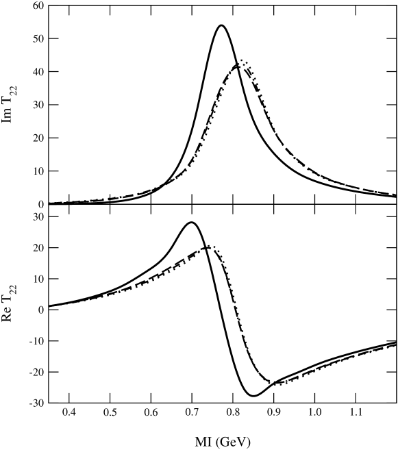
Figure 15: Real and imaginary parts of the $\pi\pi\to\pi\pi$ scattering amplitude vs invariant mass. Solid lines stand for the free case. The others correspond to the calculation at $\rho=\rho_{0}$: dashed-dotted lines for $\Lambda=1$ GeV, long dashed and dotted lines for $\Lambda=0.9,1.1$ GeV respectively.

We have also checked the dependence of the calculation on the $g^{\prime}$ Landau-Migdal parameter appearing in eq. (16). The results of this check are presented in Fig. 16, in which we show the real and imaginary parts of the scattering amplitude at $\rho=\rho_{0}$. The free case is also displayed for reference. The effects of a varying $g^{\prime}$ are noticeable in the resonance region whereas the results are insensitive for lower and higher energies. Neither the position of the resonance nor its width are much changed with variations of $g^{\prime}$ in the standard range of values $[0.6,0.8]$. We find a fluctuation of the peak position of around 3 % of the total mass at $\rho=\rho_{0}$.

Figure 16: The same as in Fig. 15 for $\rho=\rho_{0}$ and several values of $g^{\prime}$. Dashed-doted lines stand for $g^{\prime}=0.7$, long dashed and dotted lines being for $g^{\prime}=0.6,0.8$ respectively.

The results on the mass shift presented so far are in qualitative agreement with other works which find a moderate shift of the $\rho$ meson mass to higher energies at finite densities by using different approaches [16, 18].

The treatment of the $\Delta(1232)$ resonance is another issue with remarkable impact on the spectral behaviour of the $\rho$ meson in nuclear matter. The works of refs. [16, 18] where the main ingredient is the medium pion selfenergy mostly driven by the coupling to $\Delta-h$ excitations find also a broadening of the $\rho$ meson. We have found that the shape of the spectral distribution at low energies depends significantly on the $\Delta$ resonance properties specially its decay width. For instance, a simplified treatment in which a constant width is assumed gives a bump at around 500 MeV for $\rho\gtrsim\rho_{0}$. This bump disappears when an energy dependent width is used (see also [8], Fig. 3.13). Nonetheless, in some calculations having explicit energy dependence on the $\Delta$ width the bump appearing at low energies in the spectral function of the $\rho$ meson, although weakened, still remains.

Next we include in the calculation the $N^{*}(1520)$ contribution to the $\rho$ meson selfenergy in nuclear matter, as described in section 4. Our model does not try to be complete since many other resonances should be included. A much detailed work along these lines can be found in ref. [22]. Our aim is simply to estimate the effect of these type of decay channels on our previous results. The $\pi\pi$ amplitude is plotted in Fig. 17 for $\rho=\rho_{0}$ with and without the $N^{*}-h$ contribution, together with the free case for reference. The possibility of exciting a $N^{*}-h$ pair is reflected in the structure arising in the amplitude around $550$ MeV. As a consequence a sizeable amount of strength appears at energies below the $\rho$ meson mass. Our results agree qualitatively with other works in which the $\rho$ meson is allowed to couple to baryonic resonances [22, 25].

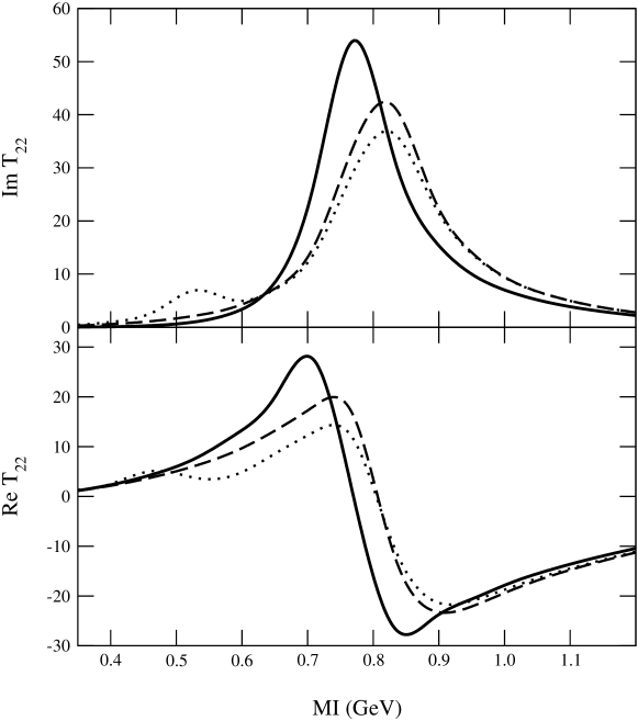
Figure 17: Real and imaginary parts of the $\pi\pi\to\pi\pi$ scattering amplitude. Long dashed (dotted) lines correspond to the results without (with) the effects of the coupling $\rho NN^{*}$ at $\rho=\rho_{0}$, and solid lines stand for the free case.

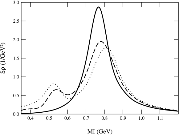
Figure 18: Spectral function of the $\rho$ meson for several values of nuclear matter density. Lines are as follows: solid, dashed and dotted stand respectively for $\rho=0$, $\rho_{0}/2$ and $\rho_{0}$.

The same behaviour discussed above is reflected in the in-medium spectral function $S_{\rho}=-\frac{1}{\pi}$Im$D_{\rho}$, which we show in Fig. 18 for the free case and several values of nuclear matter density. The first effect to be commented is that the peak of the $\rho$ distribution broadens substantially as the density is increased, its width being about 200 MeV for $\rho=\rho_{0}$. This is accompanied by a clear shift of the position of the resonance to higher energies (in agreement with many other works, see [8] for reference) that amounts, as reported before, to about $30-40$ MeV for normal nuclear matter density. Together with the $\rho$ peak we can observe a resonant structure corresponding to the excitation of the $N^{*}(1520)$ appearing around 500-550 MeV. This increases noticeably the amount of strength towards low energies, which goes in the right direction in what concerns the description of dilepton radiation spectra in that energy region [8]. The strength of the $N^{*}(1520)$ peak increases with density, which is expected since this is an effect linear in density in our model. It is also noticeable that the position of this structure is slightly pushed downwards in energy with increasing density, as a consequence of the interference with the other contributions to the $\rho$ selfenergy. In this respect we agree with refs. [24, 25] where it was pointed out that because of the coupling to baryon resonances, the in medium vector meson strength is split into a meson like mode, which is pushed up in energy and a resonance-hole like mode, which is pushed down in energy.

The results would change if one takes into account that the properties of baryonic resonances depend themselves on the rho meson medium spectral function, as it is indeed the case for the $N^{*}(1520)$ since it decays, for instance, into $N\rho[\pi\pi]$. Therefore a selfconsistent treatment is advisable. This has been done in [22], where a melting of both $N^{*}$ and $\rho$ meson structures is found at high densities so that none of them are distinguishable any longer. As a consequence, much strength is spread to lower invariant masses. Note however that this result cannot be extrapolated directly to our case since we obtain a weaker contribution of the $N^{*}-h$ excitation and our in-medium $\rho$ is also narrower than in [22].

Our results reflect the most important characteristics of the medium corrections and these are shared qualitatively by many other works in which different approaches to the problem have been used [12, 16, 17, 18, 22, 25].

6 Summary

We have analyzed the problem of the $\rho$ properties in a nuclear medium from a new perspective, using a chiral unitary framework to describe the $\rho$ meson in free space and in the medium.

The approach starts from the lowest order chiral lagrangian involving the pseudoscalar mesons plus those lagrangians coupling vector mesons to pseudoscalar mesons. The unitarization for meson-meson scattering is done following closely the idea of the $N/D$ method in coupled channels and leads to an iteration of the tree level diagrams obtained from the chiral lagrangians plus the exchange of bare vector mesons. The free parameters of the theory are obtained by matching the results to those of chiral perturbation theory for the $\pi$ and $K$ form factors plus the position of the $\rho$ peak. Once this is done the theory reproduces the experimental form factors and the scattering amplitudes in the vector sector with high accuracy up to $1.2$ GeV.

The treatment of the $\rho$ in the medium has led us to modify the previous approach, which relies upon the on-shell amplitudes provided by the lagrangians and dimensional regularization, in order to properly incorporate pion selfenergies and vertex corrections in a gauge invariant way. Whereas in vacuum it has been found that a formalism keeping tadpole diagrams and full off-shell dependence of the $\rho\pi\pi$ vertex is equivalent to the one followed in ref. [32] where only the on shell part of the $\rho\pi\pi$ vertex is kept and no tadpole diagrams are considered, in the medium one should explicitly include tadpole terms in order to preserve gauge invariance.

The inclusion of medium effects proceeds by dressing the pion propagators with a proper selfenergy and including vertex corrections. In this way the main $\rho$ decay channel into $\pi\pi$ is modified and new decay channels are opened. The main visible effect of the nuclear medium is a broadening of the $\rho$ width as the nuclear density increases. Simultaneously we observe that there is a small shift of the peak to higher energies moderately dependent on the uncertainties of the pion selfenergy.

We have also added another source of medium $\rho$ renormalization including the coupling of the $\rho$ to the $N^{*}(1520)-h$ component. This part is not novel and has been studied elsewhere, but we include it for completeness in order to show how our previous results are affected by this channel. We observe that an important source of strength appears in the $\rho$ spectral function at low energies and that the previous peak of the $\rho$ distribution is slightly pushed to higher energies. Yet the global effect is still a shift of the $\rho$ spectral function peak to higher energies of about $30-40$ MeV at $\rho=\rho_{0}$. Our results would thus agree with those where there is not much shift of the $\rho$ peak but however produce an extra strength in the isovector-vector channel at lower energies than the free $\rho$ mass, although there are quantitative differences.

Acknowledgments

We acknowledge partial financial support from the DGICYT under contract BFM2000-1326 and from the EU TMR network Eurodaphne, contract no. ERBFMRX-CT98-0169. D. C. thanks financial support from MCYT.

Appendix: Formulae for the $N^{*}-h$ Lindhard function

We give the analytic expression for the Lindhard function [37] corresponding to the $N^{*}-h$ excitation, quoted in eq. (4):

$$U_{N^{*}}(P^{0},\vec{P};\rho)=\frac{3}{2}\rho\frac{M_{N^{*}}}{Pk_{F}}\bigg{[}z+\frac{1}{2}(1-z^{2})\log\frac{z+1}{z-1}+z_{c}+\frac{1}{2}(1-z_{c}^{2})\log\frac{z_{c}+1}{z_{c}-1}\bigg{]},$$ (62)

where $k_{F}$ is the Fermi momentum, and here $P$ stands for the modulus of $\vec{P}$. Terms depending on $z$, $z_{c}$ come from direct and crossed diagrams, respectively. These functions are defined as

$$z = \frac{M_{N^{*}}}{Pk_{F}}\bigg{[}P^{0}-\omega_{R}-\frac{P^{2}}{2M_{N^{*}}}+\frac{i}{2}\Gamma(P^{0},\vec{P})\bigg{]}$$

$$z_{c} = \frac{M_{N^{*}}}{Pk_{F}}\bigg{[}-P^{0}-\omega_{R}-\frac{P^{2}}{2M_{N^{*}}}+\frac{i}{2}\Gamma(-P^{0},\vec{P})\bigg{]},$$ (63)

with $\omega_{R}=M_{N^{*}}-M_{N}$. Eq. (Appendix: Formulae for the $N^{*}-h$ Lindhard function) already includes the information of the $N^{*}$ decay width, which can be found in [38].

The limit of eq. (62) when $\vec{P}\to\vec{0}$ is given by

$$U_{N^{*}}(P^{0},\vec{0};\rho)=\rho\bigg{[}\frac{1}{P^{0}-\omega_{R}+\frac{i}{2}\Gamma(P^{0},\vec{0})}+\frac{1}{-P^{0}-\omega_{R}}\bigg{]},$$ (64)

and it is the expression that we use in our calculation as we stay in the CM frame of the $\rho$ meson.

Appendix 2: Other medium corrections not included in the text

In section 3 we have described how the presence of nuclear matter modifies the propagation of the $\rho$ meson by modifying the properties of the pionic cloud. In addition to the pion selfenergy, a set of diagrams involving the $\rho\pi NN$ contact term were also considered to preserve gauge invariance (see Fig. 7). Minimal substitution, which provides the interaction lagrangians for the mesons and baryons involved [17, 18], gives rise to some other diagrams that we have not included in the text because (i) they are higher powers of density (in the calculation only corrections of order $\rho$ are considered), (ii) they vanish for vanishing $\rho$ momentum or because of symmetry reasons, or (iii) they are negligible compared to other corrections. Now we focus on some of them and outline the derivation of some expressions that lead to our conclusions. For this purpose we classify the graphs in two sets, depending on the number of pion propagators (zero or one pionic lines), as it is shown in Fig. 19.

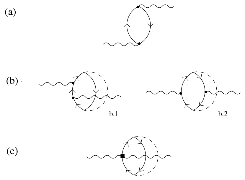
Figure 19: Medium correction graphs not included in the calculation: sets (a) and (b) involving zero and one pion lines. $\rho NN$, $\rho\Delta\Delta$ vertices are displayed as dots.

No pion lines

The first vanishing contribution corresponds to the diagram labelled as 19a, in which a $\rho$ meson directly couples to a $p-h$ excitation. This mechanism does not contribute for a $\rho$ meson at rest, since then both the particle and the hole have the same momentum. The similar diagram with $\Delta-h$ excitation involves a vanishing vertex in the non relativistic approximation, for a $\rho$ at rest.

One pion line

Here we distribute the graphs in three subsets: both $\rho$ mesons coupled to either a particle or a hole line (Fig. 19b.1), one $\rho$ meson line attached to the particle line and the other one to the hole line (Fig. 19b.2) and both $\rho$ mesons involved in a $\rho\rho NN$ contact vertex (Fig. 19c).

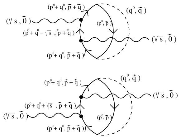
Figure 20: Momentum labelling of the diagram with two $\rho$ mesons coupled to the particle line.

Let us calculate the contribution of diagrams 19b.1. to the $\rho$ meson selfenergy. We focus on the case in which both incoming and outgoing $\rho$ mesons are coupled to the particle line (in Fig. 20 the momentum labelling is shown). Applying the Feynman rules derived from the interaction lagrangians of [18] we get the following expression:

$$-i\Pi^{ij}_{(b.1)} = -i\delta^{ij}K\int\frac{d^{4}q}{(2\pi)^{4}}(\vec{q}\,^{2})^{2}D(q)\int\frac{d^{4}p}{(2\pi)^{4}}\bigg{\{}G_{h}(p)G_{p}^{2}(p+q)G_{p}(p^{0}+q^{0}+\sqrt{s},\vec{p}+\vec{q})+{}$$ (65)

$${}G_{h}(p)G_{p}^{2}(p+q)G_{p}(p^{0}+q^{0}-\sqrt{s},\vec{p}+\vec{q})\bigg{\}}$$

where $G_{p}$ ($G_{h}$) stands for the propagator of a particle (hole) and $K=(\frac{f_{N}}{m_{\pi}})^{2}g_{\rho}^{2}(\frac{1}{M_{N}})^{2}$. In obtaining the previous expression, the $\rho NN$ vertices provide a $(\vec{p}+\vec{q})_{i}(\vec{p}+\vec{q})_{j}$ factor. The terms linear and quadratic in $\vec{p}$, when performing the integration over the momenta in the fermionic loop give rise to contributions of order $\rho^{\frac{4}{3}}$ and higher powers in the nuclear density. We neglect those contributions and then eq. (65) follows. This result can be expressed in terms of the ordinary Lindhard functions. The product of fermion propagators in eq. (65) can be rewritten as

$$G_{h}(p)G_{p}^{2}(p+q)G_{p}(p^{0}+q^{0}+\sqrt{s},\vec{p}+\vec{q})={}$$

$${}\frac{\partial}{\partial\alpha}\bigg{\{}\frac{1}{\sqrt{s}+\alpha}\bigg{[}G_{h}(p)G_{p}(p^{0}+q^{0}-\alpha,\vec{p}+\vec{q})-G_{h}(p)G_{p}(p^{0}+q^{0}+\sqrt{s},\vec{p}+\vec{q})\bigg{]}\bigg{\}}$$

$$G_{h}(p)G_{p}^{2}(p+q)G_{p}(p^{0}+q^{0}-\sqrt{s},\vec{p}+\vec{q})={}$$ (66)

$${}\frac{\partial}{\partial\alpha}\bigg{\{}\frac{-1}{\sqrt{s}-\alpha}\bigg{[}G_{h}(p)G_{p}(p^{0}+q^{0}-\alpha,\vec{p}+\vec{q})-G_{h}(p)G_{p}(p^{0}+q^{0}-\sqrt{s},\vec{p}+\vec{q})\bigg{]}\bigg{\}}$$

where the limit $\alpha\to 0$ is assumed. Commutation of this limit and the $\partial_{\alpha}$ derivative with the integration over the fermionic loop momenta allows us to write

$$-i\Pi^{ij}_{(b.1)}=\delta^{ij}\frac{K}{2}\int\frac{d^{4}q}{(2\pi)^{4}}(\vec{q}\,^{2})^{2}D(q)\frac{1}{s}\bigg{[}\bar{U}_{N}(q^{0}+\sqrt{s},\vec{q})+\bar{U}_{N}(q^{0}-\sqrt{s},\vec{q})-2\bar{U}_{N}(q)\bigg{]}$$ (67)

where the $\bar{U}$ function, the Lindhard function for a forward propagating $p-h$ bubble, stands for

$$\bar{U}_{N}(q)=-2i\int\frac{d^{4}p}{(2\pi)^{4}}G_{h}(p)G_{p}(p+q)$$ (68)

and satisfies

$$2\,[\bar{U}_{N}(q^{0},\vec{q})+\bar{U}_{N}(-q^{0},\vec{q})]=U_{N}(q^{0},\vec{q}).$$ (69)

We have compared numerically the size of this contribution to any of the ones included in Fig. 6 and we find that it is around a hundred times smaller in the range of invariant mass under study. Including this contribution in the calculation has no visible effect and therefore we neglect it, and so we do with the terms containing $\Delta$ baryons instead of nucleons.

In this derivation we have neglected all terms linear or quadratic in the hole momentum, since they generate contributions of higher order in density. Following this criterium, we can discard other contributions from diagrams with a $\rho$ meson coupled to a hole line. In particular this is the case of the partners of the graphs shown of Fig. 20, with both $\rho$ mesons coupled to the hole line. The same happens to the diagrams of the type of the one shown in Fig. 19b.2.

We are left with the evaluation of the $\rho\rho\pi\pi$ vertex correction shown in Fig. 19c, where although not displayed, the $\rho\rho NN$ vertex can also be inserted in the hole line. The momentum labelling follows the one in Fig. 20. Using the Feynman rule for the $\rho\rho NN$ vertex derived in section 3.6.3 we have

$$-i\Pi^{ij}=-ig_{\rho}^{2}\frac{3}{M_{N}}\bigg{(}\frac{f_{N}}{m_{\pi}}\bigg{)}^{2}\delta^{ij}\int\frac{d^{4}q}{(2\pi)^{4}}\vec{q}\,^{2}D(q)\int\frac{d^{4}p}{(2\pi)^{4}}G(p)G(p+q)^{2},$$ (70)

where here $G(p)$ denotes the whole nucleon propagator with both the particle and the hole pieces. It is possible to rewrite $G(p+q)^{2}$ as

$$G(p+q)^{2}=\partial_{\alpha}G(p^{0}+q^{0}-\alpha,\vec{p}+\vec{q}),$$ (71)

with $\alpha\to 0$. The integration of the fermionic loop is then given by

$$I=\int\frac{d^{4}p}{(2\pi)^{4}}G(p)G(p+q)^{2}=\partial_{\alpha}\int\frac{d^{4}p}{(2\pi)^{4}}G(p)G(p^{0}+q^{0}-\alpha,\vec{p}+\vec{q})=$$

$$\frac{i}{4}\partial_{\alpha}U(q^{0}-\alpha,\vec{q})|_{\alpha=0},$$ (72)

which is an odd function of $q^{0}$ since the Lindhard function is even in $q^{0}$. As a consequence the $dq^{0}$ integration vanishes and the contribution of these terms is null. Similar arguments for the case of a $\Delta$ in the particle line also lead to a null contribution.

References

- [1] G. Agakishiev et al. [CERES Collaboration], Phys. Rev. Lett. 75 (1995) 1272.
- [2] B. Lenkeit et al. [CERES-Collaboration], Nucl. Phys. A661 (1999) 23 [nucl-ex/9910015].
- [3] K. Filimonov et al. [CERES/NA45 Collaboration], arXiv:nucl-ex/0109017.
- [4] R. J. Porter et al. [DLS Collaboration], Phys. Rev. Lett. 79 (1997) 1229 [nucl-ex/9703001].
- [5] K. Ozawa et al. [E325 Collaboration], Phys. Rev. Lett. 86 (2001) 5019 [nucl-ex/0011013].
- [6] J. Friese [HADES Collaboration], Prog. Part. Nucl. Phys. 42 (1999) 235.
- [7] E. L. Bratkovskaya, W. Cassing and U. Mosel, Nucl. Phys. A 686 (2001) 568 [arXiv:nucl-th/0008037].
- [8] R. Rapp and J. Wambach, Adv. Nucl. Phys. 25 (2000) 1 [hep-ph/9909229].
- [9] G. E. Brown and M. Rho, Phys. Rev. Lett. 66 (1991) 2720.
- [10] T. Hatsuda and S. H. Lee, Phys. Rev. C46 (1992) 34.
- [11] S. Leupold, W. Peters and U. Mosel, Nucl. Phys. A628 (1998) 311 [nucl-th/9708016].
- [12] F. Klingl, N. Kaiser and W. Weise, Nucl. Phys. A624 (1997) 527 [hep-ph/9704398].
- [13] S. Mallik and A. Nyffeler, Phys. Rev. C 63 (2001) 065204 [hep-ph/0102062].
- [14] M. Asakawa, C. M. Ko, P. Levai and X. J. Qiu, Phys. Rev. C46 (1992) 1159.
- [15] M. Asakawa and C. M. Ko, Phys. Rev. C48 (1993) 526.
- [16] G. Chanfray and P. Schuck, Nucl. Phys. A555 (1993) 329.
- [17] M. Herrmann, B. L. Friman and W. Norenberg, Nucl. Phys. A560 (1993) 411.
- [18] M. Urban, M. Buballa, R. Rapp and J. Wambach, Nucl. Phys. A641 (1998) 433 [nucl-th/9806030].
- [19] M. Urban, M. Buballa and J. Wambach, Nucl. Phys. A673 (2000) 357 [nucl-th/9910004].
- [20] W. Broniowski, W. Florkowski and B. Hiller, nucl-th/0103027.
- [21] R. Rapp, G. Chanfray and J. Wambach, Nucl. Phys. A617 (1997) 472 [hep-ph/9702210].
- [22] W. Peters, M. Post, H. Lenske, S. Leupold and U. Mosel, Nucl. Phys. A632 (1998) 109 [nucl-th/9708004].
- [23] M. Post, S. Leupold and U. Mosel, Nucl. Phys. A 689 (2001) 753 [nucl-th/0008027].
- [24] B. Friman, Acta Phys. Polon. B 29 (1998) 3195 [nucl-th/9808071].
- [25] M. Lutz, B. Friman and G. Wolf, Nucl. Phys. A661 (1999) 526.
- [26] J. A. Oller, E. Oset and J. R. Pelaez, Phys. Rev. D59 (1999) 074001 [hep-ph/9804209].
- [27] H. C. Chiang, E. Oset and M. J. Vicente-Vacas, Nucl. Phys. A644 (1998) 77 [nucl-th/9712047].
- [28] E. Oset and M. J. Vicente Vacas, Nucl. Phys. A678 (2000) 424 [nucl-th/0004030].
- [29] R. Rapp et al., Phys. Rev. C59 (1999) R1237 [nucl-th/9810007].
- [30] M. J. Vicente Vacas and E. Oset, Phys. Rev. C60 (1999) 064621 [nucl-th/9907008].
- [31] J. A. Oller and E. Oset, Nucl. Phys. A 620 (1997) 438 [Erratum-ibid. A 652 (1997) 407] [arXiv:hep-ph/9702314].
- [32] J. A. Oller, E. Oset and J. E. Palomar, Phys. Rev. D 63 (2001) 114009 [hep-ph/0011096].
- [33] J. Gasser and H. Leutwyler, Nucl. Phys. B250 (1985) 465, 517, 539.
- [34] G. Ecker, J. Gasser, H. Leutwyler, A. Pich and E. de Rafael, Phys. Lett. B223 (1989) 425; G. Ecker, J. Gasser, A. Pich and E. de Rafael, Nucl. Phys. B321 (1989) 311.
- [35] J. A. Oller and E. Oset, Phys. Rev. D60 (1999) 074023.
- [36] E. Oset and A. Ramos, Nucl. Phys. A 679 (2001) 616 [nucl-th/0005046].
- [37] E. Oset, P. Fernandez de Cordoba, L. L. Salcedo and R. Brockmann, Phys. Rep. 188, 79 (1990).
- [38] J. A. Gomez Tejedor, F. Cano and E. Oset, Phys. Lett. B379 (1996) 39.
- [39] Y. Koike and A. Hayashigaki, Prog. Theor. Phys. 98 (1997) 631 [nucl-th/9609001].
- [40] K. Saito, K. Tsushima and A. W. Thomas, Phys. Rev. C56 (1997) 566 [nucl-th/9703011].
- [41] P. Maris, C. D. Roberts and S. M. Schmidt, Phys. Rev. C57 (1998) 2821 [nucl-th/9801059].
- [42] K. Sakamoto, M. Nakai, H. Kouno, A. Hasegawa and M. Nakano, Int. J. Mod. Phys. E9 (2000) 169 [nucl-th/9909054].