1 Introduction

With results from the SAMPLE experiment available [1], there is now great interest in parity-violating electron-deuteron scattering. The SAMPLE Collaboration measures at Bates the longitudinal asymmetry in polarized quasi-elastic electron scattering on the proton [1] and deuteron [2]. The asymmetries are sensitive to the nucleon’s strange magnetic and axial form factors. If other effects are under control, the two measurements can be used to determine the values of the form factors at $|Q^{2}|=0.1$ GeV². Neglecting two-nucleon current effects, preliminary results are in disagreement with theoretical estimates, in particular for the axial contribution [3]. The purpose of the work presented here is to compute a theoretical value for the deuteron asymmetry including two-nucleon currents.

Neutral charge and current one-nucleon operators are well known (see, for example, Ref. [4]). The contribution of such operators to the asymmetry was computed at various momentum transfers in Ref. [5]. Several theoretical issues were studied in detail. For the kinematical region relevant to SAMPLE, final-state interactions were found to be important. It was also found that (except for very low momentum transfers) the asymmetry in the vicinity of the quasi-elastic peak is fairly independent of the choice of two-nucleon ($N$$N$) potential.

Two-nucleon charge and current operators have also been studied to some extent. Heavy-meson exchange contributions were considered in Ref. [6]. They were shown to be unimportant in a calculation of the asymmetry that neglected final-state interactions. In Ref. [7], an impulse approximation modified to incorporate gauge invariance was employed. The effects of parity-violating $N$$N$ interactions on the deuteron wave function were found to be small. Pion-exchange currents were included in the computation of the asymmetry, but only in electromagnetic sector.

In the present work we extend these earlier calculations. The leading currents are calculated in Chiral Perturbation Theory (ChPT) [8, 9] supplemented by a successful phenomenological model [10]. The one-nucleon currents considered here include phenomenological form factors and have the same form as those in Ref. [4]. We also consider pion-exchange currents in both electromagnetic and weak contributions, as well as effects from heavier mesons, evaluated using the Riska prescription [11]. The asymmetry is calculated with deuteron and final-state wave functions obtained from a realistic potential, the Argonne $v_{18}$ model [12].

We present results for the kinematical region of interest to SAMPLE. (Our calculation can be repeated at other momentum transfers, such as those of the planned SAMPLE-Lite experiment [13] and JLab’s G0 experiment [14].) We verify that when two-nucleon effects are turned off, our results are in agreement with those of Ref. [5]. We study the effects of two-body currents on the asymmetry, both near the quasi-elastic peak where one-body processes should dominate, and away from the quasi-elastic peak where these two-body currents could be important. We are able to confirm that most of the two-nucleon contributions to the asymmetry are due to currents of pion range. Our results show that near the quasi-elastic peak two-body currents give a small contribution to the asymmetry. Away from the peak, they become more important, and can increase the magnitude of the asymmetry by as much as 3%. We find that the contribution to the asymmetry associated with the electromagnetic-axial current interference response function is about 20%. The overall effect of two-nucleon currents on the data of the SAMPLE experiment is indeed small but not negligible, and is being incorporated in the data analysis [3].

A summary of the relevant formulas for the calculation of the asymmetry is given in Sec. 2. Section 3.1 contains the one- and two-body electromagnetic currents, and Sec. 3.2 contains the one- and two-body neutral weak currents. The connection between our phenomenological approach and ChPT can be found in Sec. 4, while the numerical computation of the asymmetry is described in Sec. 5. Results and conclusions are presented in Sec. 6.

2 The Parity-Violating Asymmetry

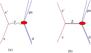
Parity-violating electron-nucleus scattering results from interference of amplitudes associated with photon and $Z^{0}$ exchanges, shown in Fig. 1. The initial and final electron (nucleus) four-momenta are labelled by $k^{\mu}$ and $k^{\prime\mu}$ ($P^{\mu}$ and $P^{\prime\mu}$), respectively, while the four-momentum transfer $Q^{\mu}$ is defined as $Q^{\mu}\equiv k^{\mu}-k^{\prime\mu}\equiv(\omega,{\bf q})$. The amplitudes for the processes in Fig. 1 are then given by [15]

$$M=-\frac{4\pi\alpha}{Q^{2}}(M^{\gamma}+M^{Z})\ ,$$ (1)

$$M^{\gamma}=\overline{u}^{\,\prime}\gamma^{\sigma}u\,j^{\gamma}_{\sigma,fi}\ ,$$ (2)

$$M^{Z}=\frac{1}{4\pi\sqrt{2}}\frac{G_{\mu}Q^{2}}{\alpha}\overline{u}^{\,\prime}\gamma^{\sigma}(g_{V}^{(e)}+g_{A}^{(e)}\gamma_{5})u\,j^{Z}_{\sigma,fi}\ ,$$ (3)

where $\alpha$ and $G_{\mu}$ are the fine-structure constant and Fermi constant for muon decay, respectively, $g_{V}^{(e)}=-1+4\,{\rm sin}^{2}\theta_{W}$ and $g_{A}^{(e)}=1$ are the Standard Model values for the neutral-current couplings to the electron given in terms of the Weinberg angle $\theta_{W}$, $u$ and $u^{\prime}$ are the initial and final electron spinors, and $j^{\gamma,\sigma}_{fi}$ and $j^{Z,\sigma}_{fi}$ denote matrix elements of the electromagnetic and weak neutral currents, i.e.

$$j^{\gamma,\sigma}_{fi}\equiv\langle f|j^{\gamma,\sigma}(0)|i\rangle\equiv(\rho^{\gamma}_{fi}({\bf q}),{\bf j}^{\gamma}_{fi}({\bf q}))\ ,$$ (4)

and similarly for $j^{Z,\sigma}_{fi}$. Here $|i\rangle$ and $|f\rangle$ are the initial and final nuclear states. Note that in the amplitude $M^{Z}$ the $Q^{2}$ dependence of the $Z^{0}$ propagator has been ignored, since here we restricted ourselves to $|Q^{2}|\ll m_{Z}^{2}$.

Figure 1: (a) Single photon- and (b) $Z^{0}$-exchange diagrams in parity-violating quasi-elastic electron-deuteron scattering. The blobs denote the nuclear currents.

The parity-violating asymmetry in the quasi-elastic regime is given by

$$A=\Bigg{(}\frac{d\sigma^{+}}{d\Omega d\omega}-\frac{d\sigma^{-}}{d\Omega d\omega}\Bigg{)}\Bigg{/}\Bigg{(}\frac{d\sigma^{+}}{d\Omega d\omega}+\frac{d\sigma^{-}}{d\Omega d\omega}\Bigg{)}\ ,$$ (5)

where $d\sigma^{h}/d\Omega d\omega$ is the inclusive cross section for scattering of an incident electron with helicity $h=\pm 1$. It is easily seen that, to leading order,

$$A\propto\frac{\Re\,(M^{\gamma}M^{Z*})}{\mid M^{\gamma}\mid^{2}}\ .$$ (6)

Standard manipulations then lead to the following expression for the asymmetry in the extreme relativistic limit for the electron [15]

$$A=\frac{1}{2\sqrt{2}}\frac{G_{\mu}Q^{2}}{\alpha}\frac{g_{A}^{(e)}v_{L}R_{L}^{\gamma,0}+g_{A}^{(e)}v_{T}R_{T}^{\gamma,0}+g_{V}^{(e)}v_{T}^{\prime}R_{T}^{\gamma,5}}{v_{L}R_{L}^{\gamma,\gamma}+v_{T}R_{T}^{\gamma,\gamma}}\ ,$$ (7)

where the $v$’s are defined in terms of electron kinematical variables,

$$v_{L} = \frac{Q^{4}}{q^{4}}\ ,$$ (8)

$$v_{T} = {\rm tan}^{2}(\theta/2)+\frac{|Q^{2}|}{2\,q^{2}}\ ,$$ (9)

$$v_{T}^{\prime} = {\rm tan}(\theta/2)\sqrt{{\rm tan}^{2}(\theta/2)+\frac{|Q^{2}|}{q^{2}}}\ ,$$ (10)

$\theta$ being the electron scattering angle in the laboratory, while the $R$’s are the nuclear electro-weak response functions, which depend on $q$ and $\omega$, to be defined below. To this end, it is first convenient to separate the weak current $j^{Z,\sigma}$ into its vector $j^{0,\sigma}$ and axial-vector $j^{5,\sigma}$ components, and to write correspondingly

$$j^{Z,\sigma}_{fi}=j^{0,\sigma}_{fi}+j^{5,\sigma}_{fi}\equiv(\rho^{0}_{fi}({\bf q}),{\bf j}^{0}_{fi}({\bf q}))+(\rho^{5}_{fi}({\bf q}),{\bf j}^{5}_{fi}({\bf q}))\ .$$ (11)

The response functions can then be expressed as

$$R_{L}^{\gamma,{\rm a}}(q,\omega)=\overline{\sum_{i}}\sum_{f}\delta(\omega+m_{i}-E_{f})\,\Re\left[\rho^{\gamma}_{fi}({\bf q})\rho^{{\rm a}*}_{fi}({\bf q})\right]\ ,$$ (12)

$$R_{T}^{\gamma,{\rm a}}(q,\omega)=\overline{\sum_{i}}\sum_{f}\delta(\omega+m_{i}-E_{f})\,\Re\left[j^{\gamma}_{x,fi}({\bf q})j^{{\rm a}*}_{x,fi}({\bf q})+j^{\gamma}_{y,fi}({\bf q})j^{{\rm a}*}_{y,fi}({\bf q})\right]\ ,$$ (13)

$$R_{T}^{\gamma,5}(q,\omega)=\overline{\sum_{i}}\sum_{f}\delta(\omega+m_{i}-E_{f})\,\Im\left[j^{\gamma}_{x,fi}({\bf q})j^{5*}_{y,fi}({\bf q})-j^{\gamma}_{y,fi}({\bf q})j^{5*}_{x,fi}({\bf q})\right]\ ,$$ (14)

where $m_{i}$ is the mass of the target (assumed at rest in the laboratory), $E_{f}$ is the energy of the final nuclear state (in general, a scattering state), and in Eqs. (12) and (13) the superscript ${\rm a}$ is either $\gamma$ or $0$. Note that there is a sum over the final states and an average over the initial spin projection states of the target, as implied by the notation ${\overline{\sum}}_{i}$. In the expressions above for the $R$’s, it has been assumed that the three-momentum transfer ${\bf q}$ is along the $z$-axis, which defines the spin quantization axis for the nuclear states.

The model for the nuclear electro-weak currents is discussed in the next sections, while the calculation of the deuteron response functions is described in Sec. 5.

3 Electro-Weak Charge and Current Operators

3.1 Electromagnetic Operators

The nuclear charge and current operators consist of one- and two-body terms that operate on the nucleon degrees of freedom:

$$\rho^{\gamma}({\bf q}) = \sum_{i}\rho^{\gamma,1}_{i}({\bf q})+\sum_{i<j}\rho^{\gamma,2}_{ij}({\bf q})\>\>,$$ (15)

$${\bf j}^{\gamma}({\bf q}) = \sum_{i}{\bf j}^{\gamma,1}_{i}({\bf q})+\sum_{i<j}{\bf j}^{\gamma,2}_{ij}({\bf q})\>\>.$$ (16)

The one-body operators $\rho^{\gamma,1}_{i}$ and ${\bf j}^{\gamma,1}_{i}$ have the standard expressions obtained from a relativistic reduction of the covariant single-nucleon current, and are listed below for convenience. The charge operator is written as

$$\rho^{\gamma,1}_{i}({\bf q})=\rho^{\gamma,1}_{i,{\rm NR}}({\bf q})+\rho^{\gamma,1}_{i,{\rm RC}}({\bf q})\>\>,$$ (17)

with

$$\rho^{\gamma,1}_{i,{\rm NR}}({\bf q})=\epsilon_{i}\>{\rm e}^{{\rm i}{\bf q}\cdot{\bf r}_{i}}\>\>,$$ (18)

$$\rho^{\gamma,1}_{i,{\rm RC}}({\bf q})=\left(\frac{1}{\sqrt{1+|Q^{2}|/4m^{2}}}-1\right)\epsilon_{i}\>{\rm e}^{{\rm i}{\bf q}\cdot{\bf r}_{i}}-{\frac{{\rm i}}{4m^{2}}}\left(2\,\mu_{i}-\epsilon_{i}\right){\bf q}\cdot(\mbox{\boldmath$\sigma$}_{i}\times{\bf p}_{i})\>{\rm e}^{{\rm i}{\bf q}\cdot{\bf r}_{i}}\>\>,$$ (19)

where $|Q^{2}|=q^{2}-\omega^{2}>0$ is the four-momentum transfer defined earlier, and $m$ is the nucleon mass. The current operator is expressed as

$${\bf j}^{\gamma,1}_{i}({\bf q})={\frac{1}{2m}}\epsilon_{i}\>\bigl{[}{\bf p}_{i}\>,\>{\rm e}^{{\rm i}{\bf q}\cdot{\bf r}_{i}}\bigr{]}_{+}-{\frac{{\rm i}}{2m}}\mu_{i}\>{\bf q}\times\mbox{\boldmath$\sigma$}_{i}\>{\rm e}^{{\rm i}{\bf q}\cdot{\bf r}_{i}}\>\>\>,$$ (20)

where $[\cdots\,,\,\cdots]_{+}$ denotes the anticommutator. The following definitions have been introduced:

$$\epsilon_{i} \equiv \frac{1}{2}\left[G_{E}^{S}(|Q^{2}|)+G_{E}^{V}(|Q^{2}|)\tau_{z,i}\right]\>\>,$$ (21)

$$\mu_{i} \equiv \frac{1}{2}\left[G_{M}^{S}(|Q^{2}|)+G_{M}^{V}(|Q^{2}|)\tau_{z,i}\right]\>\>,$$ (22)

and ${\bf p}$, $\sigma$, and $\tau$ are the nucleon’s momentum, Pauli spin and isospin operators, respectively. The two terms proportional to $1/m^{2}$ in $\rho^{\gamma,1}_{i,{\rm RC}}$ are the well known Darwin-Foldy and spin-orbit relativistic corrections [16], respectively. The dipole parametrization is used for the isoscalar ($S$) and isovector ($V$) combinations of the electric and magnetic nucleon form factors (including the Galster form for the electric neutron form factor [17]).

The most important features of the two-body parts of the electromagnetic current operator are summarized below. The reader is referred to Refs. [18, 19, 20] for a derivation and listing of their explicit expressions.

3.1.1 Two-body current operators

The two-body current operator has “model-independent” and “model-dependent” components, in the classification scheme of Riska [11]. The model-independent terms are obtained from the two-nucleon interaction (in the present study the Argonne $v_{18}$ interaction [12] is employed), and by construction satisfy current conservation with it. The leading operator is the isovector “$\pi$-like” current obtained from the isospin-dependent spin-spin and tensor interactions. The latter also generate an isovector “$\rho$-like” current, while additional model-independent isoscalar and isovector currents arise from the isospin-independent and isospin-dependent central and momentum-dependent interactions. These currents are short-ranged and numerically far less important than the $\pi$-like current.

The model-dependent currents are purely transverse and therefore cannot be directly linked to the underlying two-nucleon interaction. The present calculation includes the isoscalar $\rho\pi\gamma$ and isovector $\omega\pi\gamma$ transition currents as well as the isovector current associated with excitation of intermediate $\Delta$-isobar resonances (for the values of the various coupling constants and cutoff masses in the monopole form factors at the meson-baryon vertices, see Ref. [21]). Among the model-dependent currents, those associated with the $\Delta$-isobar are the most important ones. In the present calculation, these currents are treated within the static $\Delta$ approximation. While this is sufficiently accurate for our purposes here, it is important to realize that such an approach can lead to a gross overestimate of $\Delta$ contributions in electro-weak transitions (see Refs. [22, 23, 24] for a discussion of this issue within the context of neutron and proton radiative captures on deuteron and ³He, and the proton weak capture on ³He).

Finally, it is worth pointing out that the contributions associated with the $\rho\pi\gamma$, $\omega\pi\gamma$ and $\Delta$-excitation mechanisms are, in the regime of low to moderate momentum-transfer values of interest here ($q\leq 2$ fm^-1), typically much smaller than those due to the leading model-independent $\pi$-like current [25].

3.1.2 Two-body charge operators

While the main parts of the two-body currents are linked to the form of the two-nucleon interaction through the continuity equation, the most important two-body charge operators are model-dependent, and should be considered as relativistic corrections. Indeed, a consistent calculation of two-body charge effects in nuclei would require the inclusion of relativistic effects in both the interaction models and nuclear wave functions. There are nevertheless rather clear indications for the relevance of two-body charge operators from the failure of the impulse approximation in predicting the deuteron tensor polarization observable [26], and charge form factors of the three- and four-nucleon systems [25, 27]. The model commonly used [19] includes the $\pi$-, $\rho$-, and $\omega$-meson exchange charge operators with both isoscalar and isovector components, as well as the (isoscalar) $\rho\pi\gamma$ and (isovector) $\omega\pi\gamma$ charge transition couplings, in addition to the single-nucleon Darwin-Foldy and spin-orbit relativistic corrections. The $\pi$- and $\rho$-meson exchange charge operators are constructed from the isospin-dependent spin-spin and tensor interactions (those of the Argonne $v_{18}$ here), using the same prescription adopted for the corresponding current operators.

It should be emphasized, however, that for $q\leq 2$ fm^-1 the contributions due to these two-body charge operators are very small when compared to those from the one-body operator.

3.2 Weak Operators

In the Standard Model the vector part of the neutral weak current is related to the isoscalar ($S$) and isovector ($V$) components of the electromagnetic current, denoted respectively as $j^{\gamma,\sigma}_{S}$ and $j^{\gamma,\sigma}_{V}$, via

$$j^{0,\sigma}=-2\,{\rm sin}^{2}\theta_{W}\,j^{\gamma,\sigma}_{S}+(1-2\,{\rm sin}^{2}\theta_{W})\,j^{\gamma,\sigma}_{V}\ ,$$ (23)

and therefore the associated one- and two-body weak charge and current operators are easily obtained from those given in the preceding section.

The axial charge and current operators too have one- and two-body terms. Only the axial current

$${\bf j}^{5}({\bf q})=\sum_{i}{\bf j}^{5,1}_{i}({\bf q})+\sum_{i<j}{\bf j}^{5,2}_{ij}({\bf q})\>\>$$ (24)

enters in the calculation of the asymmetry. The axial charge operator is not needed in the present work. The one-body axial current is given, to lowest order in $1/m$, by

$${\bf j}^{5,1}_{i}({\bf q})=-G_{A}(|Q^{2}|)\frac{\tau_{z,i}}{2}{\mbox{\boldmath$\sigma$}}_{i}\,{\rm e}^{{\rm i}{\bf q}\cdot{\bf r}_{i}}\ ,$$ (25)

where the nucleon axial form factor is parametrized as

$$G_{A}(|Q^{2}|)=\frac{g_{A}}{(1+|Q^{2}|/\Lambda_{A}^{2})^{2}}\ .$$ (26)

Here $g_{A}$ is the nucleon axial coupling constant, $g_{A}=1.2654$, and the cutoff mass $\Lambda_{A}$ is taken to be 1 GeV/c², as obtained from an analysis of pion electroproduction data [28] and measurements of the reaction $\nu_{\mu}\,p\rightarrow\mu^{+}\,n$ [29].

There are relativistic corrections to ${\bf j}^{5,1}$ as well as two-body contributions arising from $\pi$-, $\rho$-, $\rho\pi$-exchange mechanisms and $\Delta$ excitation [24]. All these effects, however, are neglected in the present study. The reasons for doing so are twofold: firstly, axial current contributions to the asymmetry are small, since they are proportional to the electron neutral weak coupling $g_{V}^{(e)}\simeq-0.074$ (see Eq. (7)); secondly, axial contributions from two-body operators are expected to be at the $\simeq 1$ % level of those due to the one-body operator in Eq. (25). For example, in the proton weak capture on proton at keV energies [30]–this process is induced by the charge-changing axial weak current–the $\pi$, $\rho$, $\rho\pi$, and $\Delta$ two-body operators increase the predicted one-body cross section by 1.5%. Such an estimate is expected to hold up also in the quasi-elastic regime being considered here.

4 Connection with Chiral Perturbation Theory

The purpose of this section is to relate the operators presented in Sections 3.1 and 3.2 to ChPT. We consider only up and down quarks, in which case the QCD Lagrangian has an approximate $SU(2)_{L}\times SU(2)_{R}$ chiral symmetry. This symmetry is spontaneously broken by the vacuum to the diagonal $SU(2)_{V}$ subgroup, and three pseudoscalar Goldstone bosons, the pions $\pi_{a}$, appear in the spectrum. Chiral symmetry provides important constraints on the description of low-momentum processes involving pions. In particular, it allows one to estimate the relative size of various contributions.

To accomplish this, the most general effective Lagrangian with broken $SU(2)_{L}\times SU(2)_{R}$ is constructed. This effective Lagrangian includes terms with arbitrary number of derivatives and powers of the quark masses, however higher-dimension operators are suppressed by inverse powers of the characteristic mass scale of QCD, $M_{QCD}\sim 1$ GeV. Thus pion interactions are determined as a power series in $(q,m_{\pi})/M_{QCD}$, where $q$ is the typical external three-momentum. At low energies this is a small number and hence only the lowest-order terms are considered in this paper.

We start with the $\pi\pi$ and $\pi N$ Lagrangians. Details can be found, for example, in Refs. [8, 9]. We lump the pions in a field $U=u^{2}=1+{\rm i}\mbox{\boldmath$\tau$}\cdot\mbox{\boldmath$\pi$}/f_{\pi}-\mbox{\boldmath$\pi$}^{2}/2f_{\pi}^{2}+...$, where $f_{\pi}=93$ MeV is the pion decay constant. We denote the nucleon field of velocity $v_{\mu}$ and spin $S_{\mu}$ by $N$. In order to obtain the currents required for the computation of the asymmetry we must use the proper covariant derivatives. The covariant derivatives on the pion and nucleon field are constructed in terms of external vector and axial-vector fields ${\cal V}_{\mu}$ and ${\cal A}_{\mu}$ in the usual manner. They are given by

$$D_{\mu}U=\partial_{\mu}U-{\rm i}({\cal V}_{\mu}+{\cal A}_{\mu})U+{\rm i}\,U({\cal V}_{\mu}-{\cal A}_{\mu}),\\$$ (27)

$$D_{\mu}N=\partial_{\mu}N+\frac{1}{2}[u^{\dagger},\partial_{\mu}u]N-\frac{\rm i}{2}\Bigg{[}u^{\dagger}({\cal V}_{\mu}^{(3)}+{\cal A}_{\mu}^{(3)})u+u({\cal V}_{\mu}^{(3)}-{\cal A}_{\mu}^{(3)})u^{\dagger}\Bigg{]}N-3{\rm i}\,{\cal V}_{\mu}^{(0)}N,$$ (28)

where the superscripts $(0)$ and $(3)$ denote isoscalar and isovector components. It is convenient to construct also other quantities that transform covariantly. For example,

$$a_{\mu} = {\rm i}[u^{\dagger},D_{\mu}u]_{+},$$ (29)

$$f_{\mu\nu}^{\dagger} = u^{\dagger}F_{\mu\nu}^{R}u+uF_{\mu\nu}^{L}u^{\dagger},$$ (30)

where $F_{\mu\nu}^{R,L}=\partial_{\mu}F_{\nu}^{R,L}-\partial_{\nu}F_{\mu}^{R,L}-{\rm i}[F_{\nu}^{R,L},F_{\mu}^{R,L}]$ with $F_{\mu}^{R}={\cal V}_{\mu}+{\cal A}_{\mu}$ and $F_{\mu}^{L}={\cal V}_{\mu}-{\cal A}_{\mu}$.

One can find the relation between the external fields and $Z^{0}$ or photon by considering the covariant derivative on the quark fields (see, e.g., Ref. [31]):

$${\cal A}_{\mu}=\frac{g}{2\cos\theta_{W}}\frac{\tau_{z}}{2}Z_{\mu},$$ (31)

$${\cal V}_{\mu}=\frac{g}{2\cos\theta_{W}}(\frac{\tau_{z}}{2}-2\sin^{2}\theta_{W}Q_{q})Z_{\mu}+eQ_{q}A_{\mu},$$ (32)

where $Q_{q}$ is the quark-charge matrix.

From these building blocks we can write the chiral Lagrangians,

$${\cal L}_{\pi\pi}=\frac{f_{\pi}^{2}}{4}{\rm Tr}[D_{\mu}U^{\dagger}D^{\mu}U]+\ldots,\\$$ (33)

$${\cal L}_{\pi N}=N^{\dagger}[{\rm i}\,v\cdot D+g_{A}S\cdot a]N+\frac{1}{2m}N^{\dagger}\Bigg{[}(v\cdot D)^{2}-D\cdot D-{\rm i}\,g_{A}[S\cdot D,v\cdot v]_{+}\Bigg{]}N$$

$$-\frac{\rm i}{4m}N^{\dagger}[S^{\mu},S^{\nu}]\Bigg{[}(1-\kappa_{v})f_{\mu\nu}^{\dagger}+\frac{1}{2}(\kappa_{s}-\kappa_{v}){\rm Tr}(f_{\mu\nu}^{\dagger})\Bigg{]}N+\ldots,$$ (34)

where $\kappa_{s}=-0.12$ and $\kappa_{v}=3.71$, and $\ldots$ denote terms with more derivatives and/or powers of the pion mass. One can also write down interactions containing four or more nucleon fields [9, 32], which are important for a fully consistent description of systems involving two or more nucleons. One and two-body currents can be obtained from these interactions.

4.1 Ordering

The symmetries allow an infinite number of interactions, so an ordering scheme is necessary for predictive power. We want to estimate the size of matrix elements of one- or two-body currents between $N$$N$ wave functions. These matrix elements involve: the final $N$$N$ wave function, a two-nucleon propagator, the current operator, another two-nucleon propagator, and the initial $N$$N$ wave function. Each two-nucleon propagator brings a factor $m/q^{2}$, and each loop a $q^{3}/(4\pi)^{2}$. Apart from loops in the operators themselves, matrix elements of one- and two-body operators involve, respectively, one and two loops.

Let us first consider only strong interactions between nucleons [9]. These start at ${\cal O}(q^{0}/f_{\pi}^{2})$, and most structures that appear up to ${\cal O}(q^{3}/f_{\pi}^{2}M_{QCD}^{3})$ [32] are present in the Argonne $v_{18}$ potential [12]. Use of phenomenological potentials in conjunction with currents derived in ChPT has already proven to be a successful approach [9].

Contributions to the amplitude $M^{\gamma}$ start at ${\cal O}(e^{2}m/q^{3})$ with the tree-level one-body charge operator. First corrections come in tree-level one-body currents from ${\cal O}(q/m)$ magnetic corrections in the Lagrangian. Second corrections are of two types: (i) one-loop corrections and ${\cal O}(q^{2}/M_{QCD}^{2})$ interactions in one-body currents; and (ii) tree-level two-body currents. And so on. Contributions to the amplitude $M^{Z}$ follow the same pattern, but have an extra overall factor of ${\cal O}(q^{2}/M_{Z}^{2})={\cal O}(G_{\mu}q^{2}/e^{2})$. The leading one and two-body contributions are described in Sec. 4.2 below.

Electromagnetic interactions between nucleons are clearly higher-order effects, also included in the $v_{18}$ potential. Interesting are also the contributions to the asymmetry that come not from the exchange of a $Z^{0}$ between electron and deuteron, but from $Z^{0}$ exchange between hadrons (and photon exchange between electron and deuteron). Let us denote these contributions by $M^{\gamma(Z)}$. How does $M^{\gamma(Z)}$ compare to $M^{Z}$?

Direct $Z$ exchange between nucleons is an ${\cal O}(G_{\mu})$ effect, so suppressed by ${\cal O}(G_{\mu}f_{\pi}^{2})$ compared to the strong interaction. On the other hand, the electron-deuteron interaction is ${\cal O}(e^{2}/q^{2}G_{\mu})$ larger in $M^{\gamma(Z)}$ than in $M^{Z}$. As a consequence, the contribution from $Z^{0}$ exchange between nucleons to $M^{\gamma(Z)}$ is ${\cal O}(e^{2}f_{\pi}^{2}/q^{2})$ compared to the leading contribution to $M^{Z}$. Since we are interested in $q\sim f_{\pi}$, this is $\sim e^{2}$, a small effect. Yet, we are here searching for subleading contributions. As we have seen, two-body currents in $M^{Z}$ are suppressed by ${\cal O}(q^{2}/M_{QCD}^{2})$ compared to the leading one-body effect. Thus, compared to two-body currents in $M^{Z}$, $M^{\gamma(Z)}$ can be ${\cal O}(e^{2}f_{\pi}^{2}M_{QCD}^{2}/q^{4})$; for momenta $q\sim f_{\pi}$, this is $\sim 1$. There exist also potentially larger contributions to $M^{\gamma(Z)}$. The size of the parity-violating pion-nucleon coupling might be as large as ${\cal O}(G_{\mu}f_{\pi}^{2}M_{QCD}/q)$ compared to the parity-conserving coupling [33]. In this case pion exchange in the one-body current (anapole form factor), in the potential and in the two-body current could all produce an effect ${\cal O}(M_{QCD}/q)$ compared to two-nucleon effects in direct $Z^{0}$ exchange.

Our calculation involves all contributions suppressed by ${\cal O}(q^{2}/M_{QCD}^{2})$ (and also some even more suppressed) compared to leading, except for $M^{\gamma(Z)}$. However, contributions to $M^{\gamma(Z)}$ from the parity-violating potential were already examined in Ref. [7]. Also, although not included in any deuteron calculation, the anapole form factor of the nucleon seems too small [33] to be relevant here, and it is reasonable to expect that two-body currents stemming from the parity-violating pion-nucleon coupling will be equally unimportant. (This should be eventually confirmed in an explicit calculation.) On the other hand, the leading two-body currents in the amplitude $M^{Z}$ stemming from pion exchange are being calculated here for the first time.

4.2 One- and two-body currents

Figure 2: Electromagnetic one-body diagrams. Solid lines denote nucleons, and the blob represents the one-body current.

Figure 3: Weak neutral one-body diagrams. Symbols as in Fig. 2.

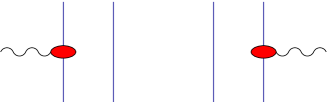
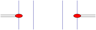
The one-body currents contributing to the processes in Fig. 1, depicted in Figs. 2 and 3, are given to ${\cal O}(eq/M_{QCD})$ by

$$\rho^{\rm a}({\bf r}) = \frac{1}{2}\sum_{i}(g_{E}^{S}+g_{E}^{V}\tau_{z,i})\delta({\bf r}-{\bf r}_{i})$$ (35)

$${\bf j}^{\rm a}({\bf r}) = \frac{1}{4m}\sum_{i}\Bigg{[}(g_{E}^{S}+g_{E}^{V}\tau_{z,i})[\delta({\bf r}-{\bf r}_{i}){\bf p}_{i}+{\bf p}_{i}\delta({\bf r}-{\bf r}_{i})]$$ (36)

$$+(g_{M}^{S}+g_{M}^{V}\tau_{z,i})\mbox{\boldmath$\nabla$}\delta({\bf r}-{\bf r}_{i})\times\mbox{\boldmath$\sigma$}_{i}\Bigg{]}$$

$$\rho^{5}({\bf r}) = -\frac{1}{4m}g_{A}\sum_{i}[\mbox{\boldmath$\sigma$}_{i}\cdot{\bf p}_{i}\delta({\bf r}-{\bf r}_{i})+\delta({\bf r}-{\bf r}_{i})\mbox{\boldmath$\sigma$}_{i}\cdot{\bf p}_{i}]\tau_{z,i}$$ (37)

$${\bf j}^{5}({\bf r}) = -\frac{1}{2}g_{A}\sum_{i}\delta({\bf r}-{\bf r}_{i})\mbox{\boldmath$\sigma$}_{i}\tau_{z,i}.$$ (38)

where ${\rm a}=\gamma$ or $0$, the coupling constants $g_{E}^{(S,V)}$ and $g_{M}^{(S,V)}$ are given in Table 1, and $g_{A}$ is the nucleon axial coupling constant. These results are in agreement with those presented in Ref. [4]. These coupling constants acquire, in higher orders, a $Q^{2}$ dependence, see Ref. [34]. In our calculation we use a phenomenological parametrization of the $Q^{2}$ dependence, as described in Secs. 3.1 and 3.2.

Form Factor	$\gamma$	$Z$
$g_{E}^{S}$	1	$-2\sin^{2}\theta_{W}$
$g_{E}^{V}$	1	$1-2\sin^{2}\theta_{W}$
$g_{M}^{S}$	$1+\kappa_{s}$	$-(1+\kappa_{s})\sin^{2}\theta_{W}$
$g_{M}^{V}$	$1+\kappa_{v}$	$(1+\kappa_{v})(1-2\sin^{2}\theta_{W})$

Table 1: Coupling constants appearing in one-body currents to ${\cal O}(eq/M_{QCD})$ in ChPT.

Note that ${\cal L}_{\pi\pi}$ contains a $\pi$-$Z^{0}$ mixing term in the form $Z\cdot\partial\pi^{0}$, which turns out to be proportional to $Q_{\mu}$, the four-momentum transfer. Its contraction with the leptonic current produces a contribution proportional to the mass of the electron. In the extreme relativistic limit for the electron under consideration here, this contribution can be neglected.

Figure 4: Electromagnetic two-body diagrams to ${\cal O}(eq^{2}/M_{QCD}^{2})$ in ChPT. Solid (dashed) lines denote nucleons (pions).

Figure 5: Weak neutral two-body diagrams to ${\cal O}(eq^{2}/M_{QCD}^{2})$ in ChPT. Symbols as in Fig. 4.

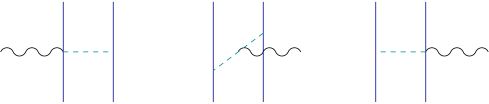
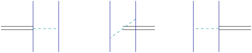
The two-body contributions to the processes shown in Fig. 1 are depicted in Figs. 4 and 5, where again contributions from $\pi$-$Z^{0}$ mixing are neglected in the extreme relativistic limit. To ${\cal O}(eq^{2}/M_{QCD}^{2})$, they are given in momentum space by

$${\bf j}^{\rm a}({\bf k}_{1},{\bf k}_{2}) = 3{\rm i}\,g_{E}^{V}(\mbox{\boldmath$\tau$}_{1}\times\mbox{\boldmath$\tau$}_{2})_{z}\Bigg{[}v_{\pi}(k_{2})\mbox{\boldmath$\sigma$}_{2}\cdot{\bf k}_{2}\mbox{\boldmath$\sigma$}_{1}-v_{\pi}(k_{1})\mbox{\boldmath$\sigma$}_{1}\cdot{\bf k}_{1}\mbox{\boldmath$\sigma$}_{2}$$ (39)

$$\hskip 78.24507pt-\frac{v_{\pi}(k_{2})-v_{\pi}(k_{1})}{{k_{1}}^{2}-{k_{2}}^{2}}({\bf k}_{1}-{\bf k}_{2})\mbox{\boldmath$\sigma$}_{1}\cdot{\bf k}_{1}\mbox{\boldmath$\sigma$}_{2}\cdot{\bf k}_{2}\Bigg{]}\ ,$$

where ${\bf k}_{i}={\bf p}^{\prime}_{i}-{\bf p}_{i}$ with ${\bf p}_{i}$ (${\bf p}_{i}^{\prime}$) denoting the initial (final) momentum of nucleon $i$. In the formula above,

$$v_{\pi}(k)=-\frac{1}{3}{\left(\frac{g_{A}}{4f_{\pi}}\right)}^{2}\frac{1}{{m_{\pi}}^{2}+k^{2}}\ .$$ (40)

Note that there is no contribution to the axial current operator or the electromagnetic charge operator. There is a contribution to the axial charge operator which, however, does not enter in the asymmetry computation. These results are in agreement with Ref. [18], where the Fourier transform of the above expressions are also given in detail.

In higher order other currents appear. There exist shorter-range currents, which are expected to be smaller than the ones from pion exchange with leading order interactions. These higher-order effects are parametrized in our calculation through the Riska prescription as outlined in Sections 3.1 and 3.2. In particular, we do not use Eq. (40) for $v_{\pi}(k)$, but the pseudoscalar component of the $v_{18}$ potential.

5 Calculation

In this section we describe the calculation of the deuteron response functions given in Eqs. (12)–(14). The deuteron wave function is written as

$$|d,M_{d}\rangle=\Bigg{[}\frac{u(r)}{r}{\cal Y}_{011}^{M_{d}}+\frac{w(r)}{r}{\cal Y}_{211}^{M_{d}}\Bigg{]}\chi_{0}^{0}\ ,$$ (41)

where the ${\cal Y}_{LSJ}^{M_{J}}$ are standard spin-angle functions, $\chi^{T}_{M_{T}}$ is a two-nucleon $T,M_{T}$ isospin state, and $u(r)$ and $w(r)$ are the S- and D-wave radial functions.

In the ²H($\vec{e},e^{\prime}$)$pn$ reaction the final state is in the continuum, and its wave function is written as

$$|{\bf q};{\bf p},SM_{S},TM_{T}\rangle={\rm e}^{{\rm i}{\bf q}\cdot{\bf R}}\,\psi_{{\bf p},SM_{S},TM_{T}}^{(-)}({\bf r})\ ,$$ (42)

where ${\bf r}\!=\!{\bf r}_{1}\!-\!{\bf r}_{2}$ and ${\bf R}\!=\!({\bf r}_{1}+{\bf r}_{2})/2$ are the relative and center-of-mass coordinates. The incoming-wave scattering-state wave function of the two nucleons having relative momentum ${\bf p}$ and spin-isospin states $SM_{S},TM_{T}$ is approximated as [35]

$$\psi_{{\bf p},SM_{S},TM_{T}}^{(-)}({\bf r}) \simeq {1\over\sqrt{\,2}}\Bigl{[}e^{{\rm i}{\bf p}\cdot{\bf r}}-(-1)^{S+T}e^{-{\rm i}{\bf p}\cdot{\bf r}}\Bigr{]}\chi_{M_{S}}^{S}\chi_{M_{T}}^{T}+{4\pi\over\sqrt{\,2}}\sum_{\scriptstyle JM_{J}\atop\scriptstyle J\leq J_{\rm max}}\sum_{LL^{\prime}}{\rm i}^{L}\,\delta_{LST}$$ (43)

$$\quad\bigl{[}Z_{LSM_{S}}^{JM_{J}}(\hat{\bf p})\bigr{]}^{*}\Biggl{[}{1\over r}u_{L^{\prime}L}^{(-)}(r;p,JST)-\delta_{L^{\prime}L}\>\>j_{L}(pr)\Biggr{]}\,{\cal Y}_{L^{\prime}SJ}^{M_{J}}\chi_{M_{T}}^{T}\ ,$$

where

$$\delta_{LST} = 1-(-1)^{L+S+T}\>\>,$$ (44)

$$Z_{LSM_{S}}^{JM_{J}}(\hat{\bf p}) = \sum_{M_{L}}\langle LM_{L},SM_{S}|JM_{J}\rangle Y_{LM_{L}}(\hat{\bf p})\>\>.$$ (45)

The $\delta_{LST}$ factor ensures the antisymmetry of the wave function, while the Clebsch-Gordan coefficients restrict the sum over $L$ and $L^{\prime}$. The radial functions $u_{L^{\prime}L}^{(-)}$ are obtained by solving the Schrödinger equation in the $JST$ channel, and behave asymptotically as

$${1\over r}u_{L^{\prime}L}^{(-)}(r;p,JST)_{\,\,{\scriptstyle\sim\atop\scriptstyle{r\to\infty}}}\,{1\over 2}\Biggl{[}\delta_{L^{\prime}L}h_{L}^{(1)}(pr)+(S_{L^{\prime}L}^{JST})^{*}h_{L^{\prime}}^{(2)}(pr)\Biggr{]}\>\>,$$ (46)

where $S_{L^{\prime}L}^{JST}$ is the $S$-matrix in the $JST$ channel and the Hankel functions are defined as $h_{L}^{(1,2)}(x)$=$j_{L}(x)\pm{\rm i}\,n_{L}(x)$, $j_{l}$ and $n_{L}$ being the spherical Bessel and Neumann functions, respectively. In the absence of interactions, $u_{L^{\prime}L}^{(-)}(r;p,JST)/r\longrightarrow\delta_{L^{\prime}L}\>\>j_{L}(pr)$, and $\psi^{(-)}({\bf r})$ reduces to an antisymmetric plane wave. Interactions effects are retained in all partial waves with $J\leq J_{\rm max}$. In the quasi-elastic regime of interest here, it is found that these interaction effects are negligible for $J_{\rm max}\!>\!7$.

The response functions are written as (only $R_{L}^{\gamma,\gamma}$ is given below for illustration)

$$R_{L}^{\gamma,\gamma}(q,\omega)=\sum_{S,T=0,1}R_{L}^{\gamma,\gamma}(q,\omega;S,T)\ ,$$ (47)

where the contributions from the individual spin-isospin states are

$$R_{L}^{\gamma,\gamma}(q,\omega;S,T)={1\over 3}\sum_{M_{d}M_{S}}\int{d{\bf p}\over(2\pi)^{3}}{1\over 2}|A^{\gamma}_{ST}({\bf q},{\bf p};M_{S}M_{d})|^{2}\delta\Bigg{(}\omega+E_{d}-\frac{q^{2}}{6\,m}-\frac{p^{2}}{m}\,\Bigg{)}\ ,$$ (48)

with $A^{\gamma}_{ST}$ defined as

$$A^{\gamma}_{ST}({\bf q},{\bf p};M_{S}M_{d})\equiv\langle{\bf q};{\bf p},SM_{S}T,M_{T}=0|\rho^{\gamma}({\bf q})|d,M_{d}\rangle\ .$$ (49)

Here $E_{d}=-2.225$ MeV is the deuteron ground-state energy, the factor 1/2 in Eq. (48) is included to avoid double counting, and the states $|d,M_{d}\rangle$ and $|{\bf q};{\bf p},SM_{S}T,M_{T}=0\rangle$ are represented by the wave functions in Eqs. (41) and (43), respectively. By integrating out the energy-conserving $\delta$-function one finds:

$$R_{L}^{\gamma,\gamma}(q,\omega;S,T)=\frac{m\,p}{48\,\pi^{2}}\sum_{M_{d},M_{S}}\int_{-1}^{+1}d({\rm cos}\theta_{\bf p})\,|A^{\gamma}_{ST}(q,p,{\rm cos}\theta_{\bf p};M_{S}M_{d})|^{2}\ ,$$ (50)

where the magnitude of the relative momentum ${\bf p}$ is fixed by $p=\sqrt{m(\omega+E_{d})-q^{2}/4}$, and $\theta_{\bf p}$ is the angle between ${\bf q}$ and ${\bf p}$. The initial- and final-state wave functions are written as vectors in the spin-isospin space of the two nucleons for any given spatial configuration ${\bf r}$. For the given ${\bf r}$ the state vector $\rho^{\gamma}({\bf q})|d,M_{d}\rangle$ is calculated with the same methods used in quantum Monte Carlo calculations of, for example, the charge and magnetic form factors of the trinucleons [25]. The ${\bf r}$ and $\theta_{\bf p}$ integrations required to calculate the amplitudes and response function are then performed by means of Gaussian quadratures.

Finally, note that, since the deuteron is a $T=0$ state, one finds

$$R^{\gamma,0}_{L}(q,\omega;S,T=0) = -2\,{\rm sin}^{2}\theta_{W}\,R^{\gamma,\gamma}_{L}(q,\omega;S,T=0)\ ,$$ (51)

$$R^{\gamma,0}_{L}(q,\omega;S,T=1) = (1-2\,{\rm sin}^{2}\theta_{W})\,R^{\gamma,\gamma}_{L}(q,\omega;S,T=1)\ ,$$ (52)

with similar relations holding between the transverse response functions.

6 Results and Conclusions

The asymmetry has been calculated at the kinematics relevant to the SAMPLE experiment. The incident electron energy was set to $E=193$ MeV. SAMPLE measures the asymmetry at four different angles ($\theta=138.4^{o},145.9^{o},154.0^{o},160.4^{o}$). Different electron final energies $E^{\prime}$ correspond to different momentum transfers $Q^{2}$, $|Q^{2}|\simeq 0.1$ GeV² in the SAMPLE experiment, which is small enough to justify the use of a non-relativistic formalism with leading interactions obtained from ChPT.

The calculated asymmetries, as functions of the electron final energy, are shown in Figs. 6, 7, 8, and 9, for the four different electron scattering angles. For each set of kinematics, the left panels display the asymmetry and the total inclusive cross section, with different curves representing one-body contributions, one- plus two-body contributions from pion-exchange currents only, and the sum of all contributions. The ratios of one- plus two-body contributions from pion only and full currents to one-body contributions for both asymmetries and cross sections are displayed in the right panels.

Figure 6: Results for scattering of an electron with incident energy $E=193$ MeV on a deuteron at rest, as function of the electron final energy $E^{\prime}$ in MeV, for a scattering angle $\theta=160.5^{o}$. Left panels: longitudinal asymmetry $|A|$ (top) and cross section $\sigma$ in fm²/MeV/sr (bottom). Shown are one-body contributions (dotted line), one- plus two-body contributions from pion-exchange currents only (dashed line), and the sum of all contributions (solid line). Right panels: ratios of one- plus two-body contributions from pion only (dashed line) and full currents (solid line) to one-body contributions for the asymmetry $|A|/|A_{1}|$ (top) and cross section $\sigma/\sigma_{1}$ (bottom).

Figure 7: Same as Fig. 6, but for $\theta=154.0^{o}$.

Figure 8: Same as Fig. 6, but for $\theta=145.9^{o}$.

Figure 9: Same as Fig. 6, but for $\theta=138.4^{o}$.

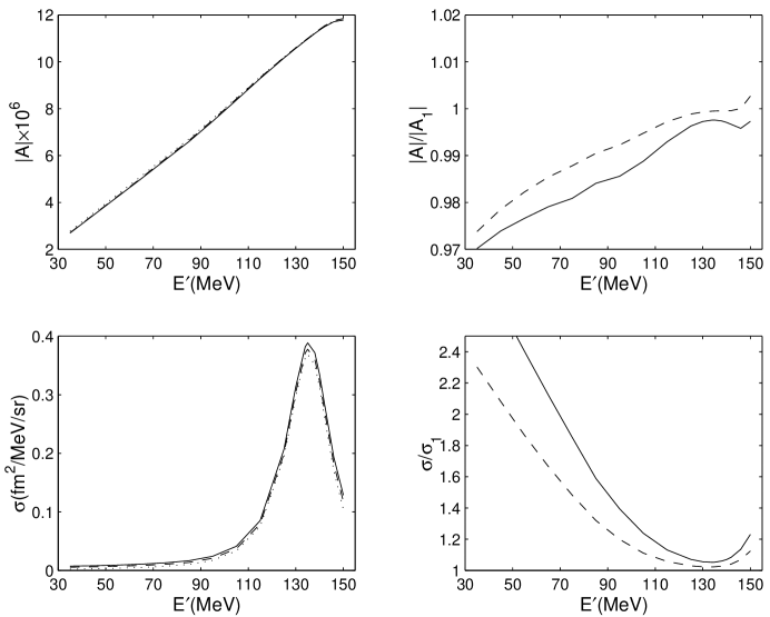
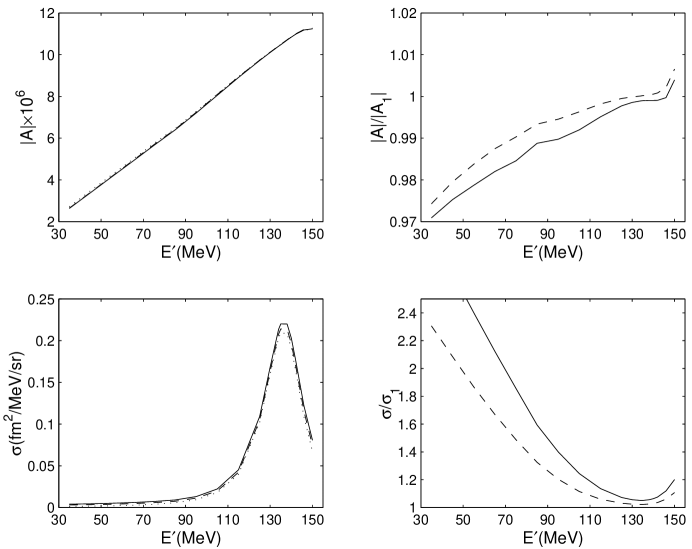
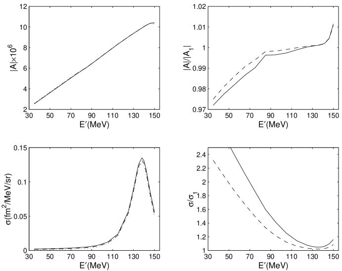
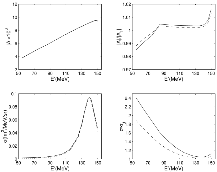
As is apparent from the figures, the results at all angles are qualitatively similar. Near the quasi-elastic peak two-body effects in the asymmetry are negligible, less than 1%, while away from the quasi-elastic peak they become relatively more important, increasing the asymmetry by at the most 3%. Note, however, that the two-body current contributions are large in the inclusive cross section, indeed dominant in the left-hand side of the quasielastic peak. In this region the contribution associated with the currents of pion range is more than 50% of the total two-body contribution.

It is interesting to examine more closely the reasons for the relative unimportance of two-body current contributions in the asymmetry. At backward angles, the expression for the asymmetry can be approximated as

$$\frac{A}{G_{\mu}Q^{2}/(2\sqrt{2}\alpha)}\simeq\frac{R_{T}^{\gamma,0}+(-1+4\,{\rm sin}^{2}\theta_{W})R_{T}^{\gamma,5}}{R_{T}^{\gamma,\gamma}}\ ,$$ (53)

where terms proportional to the longitudinal response functions are suppressed by the factor $v_{L}/v_{T}\leq 1/{\rm tan}^{2}(\theta/2)$, a small number at the angles under consideration here (note that the $R_{L}^{\gamma,{\rm a}}$ and $R_{T}^{\gamma,{\rm a}}$ response functions are of the same order of magnitude). It is useful to identify the contributions from $T=0$ and $T=1$ $pn$ final states, and to use Eqs. (51) and (52), relating the $R_{T}^{\gamma,0}(T=0,1)$ to $R_{T}^{\gamma,\gamma}(T=0,1)$. One then finds:

$$\frac{A}{G_{\mu}Q^{2}/(2\sqrt{2}\alpha)} = \frac{1-2\,{\rm sin}^{2}\theta_{W}(1+r^{\gamma,\gamma})+(-1+4\,{\rm sin}^{2}\theta_{W})\,r^{\gamma,5}}{1+r^{\gamma,\gamma}}\ ,$$ (54)

$$r^{\gamma,\gamma} = R_{T}^{\gamma,\gamma}(T=0)/R_{T}^{\gamma,\gamma}(T=1)\ ,$$ (55)

$$r^{\gamma,5} = R_{T}^{\gamma,5}(T=1)/R_{T}^{\gamma,\gamma}(T=1)\ .$$ (56)

Note that the $R_{T}^{\gamma,5}$ response function only receives contributions from $T=1$ $pn$ final states, since the current ${\bf j}^{5,1}$ is isovector. The ratio $r^{\gamma,\gamma}$ is much smaller than one, since the transverse response is predominantly isovector. For example, at $E^{\prime}=55$ MeV and $\theta=160.5^{o}$, $R_{T}^{\gamma,\gamma}(T=0)=0.769\times 10^{-5}(0.935\times 10^{-5})$ MeV^-1 and $R_{T}^{\gamma,\gamma}(T=1)=10.3\times 10^{-5}(25.9\times 10^{-5})$ MeV^-1, and hence $r^{\gamma,\gamma}=0.0748\>(0.0361)$ with one-body (full) currents. In contrast, the ratio $r^{\gamma,5}$ is of order one; again at $E^{\prime}=55$ MeV and $\theta=160.5^{o}$, $R_{T}^{\gamma,5}(T=1)=-18.3\times 10^{-5}(-26.0\times 10^{-5})$ MeV^-1, and hence $r^{\gamma,5}=-1.78\>(-1.00)$ with one-body (full) currents. However, it is multiplied by the small factor $(-1+4\,{\rm sin}^{2}\theta_{W})=-0.074$, and so the asymmetry turns out to be largely independent of nuclear structure details.

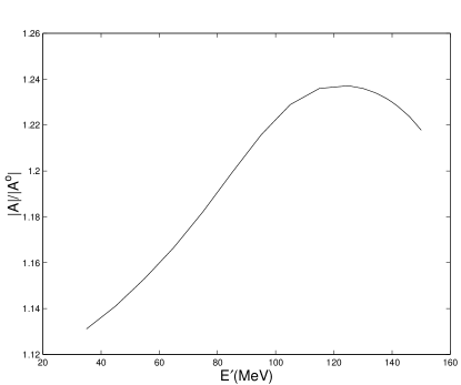
Finally, if $A^{0}$ denotes the asymmetry obtained by ignoring the contribution of the axial current, one finds

$$\frac{|A|}{|A^{0}|}=1+\frac{(-1+4\,{\rm sin}^{2}\theta_{W})\,r^{\gamma,5}}{1-2\,{\rm sin}^{2}\theta_{W}(1+r^{\gamma,\gamma})}\ .$$ (57)

The computed value for this ratio is shown in Fig. 10 for one of the kinematics of the SAMPLE experiment. The contribution of the axial current to the asymmetry is of the order of 13% to 24% throughout the kinematical range considered. Note that in Fig. 10 we have included the small contribution from the longitudinal response.

As a last remark, we should emphasize that the calculated transverse ($R_{T}^{\gamma,\gamma}$) and longitudinal ($R_{L}^{\gamma,\gamma}$) response functions –including one- and two-body operators– reproduce [36] existing Bates data [37].

Figure 10: The ratio $|A|/|A^{0}|$ where $|A|$ is the full asymmetry and $|A^{0}|$ is the asymmetry without the axial contribution for scattering of an electron with incident energy $E=193$ MeV on a deuteron at rest, as function of the electron final energy $E^{\prime}$ in MeV, for a scattering angle $\theta=160.5^{o}$.

Since we have performed the computations at the SAMPLE kinematics, the above results may be used to account for two-body current corrections in the analysis of the experimental data. The SAMPLE experiment measures a convolution of the asymmetry $A$ and the cross section $(d\sigma/d\Omega dE^{\prime})$ over a certain range of electron final energies:

$$A_{total}=\frac{\int A\left(d\sigma/d\Omega dE^{\prime}\right)dE^{\prime}}{\int\left(d\sigma/d\Omega dE^{\prime}\right)dE^{\prime}}.$$ (58)

The goal of the experiment is to extract the one-body part of $A_{total}$. To accomplish this, a model that includes only one-body contributions is used to generate the cross section. One can now use our results for the ratios of total to one-body contributions in the asymmetry and cross section to adjust for two-body effects in the experiment.

In conclusion, we have presented a fairly complete calculation of the asymmetry in quasi-elastic electron-deuteron scattering arising from $Z^{0}$ exchange. Since we find that, when the cross section is large at the quasi-elastic peak, the change in the asymmetry due to two-body currents is negligible, we expect that these two-body corrections will produce a modification in the analysis of the SAMPLE experiment at the % level, too small to affect significantly the extraction of the strange and axial form factors of the nucleon. It remains to be examined whether the same holds for effects from $Z^{0}$ exchange that manifest themselves within the two-nucleon system through the parity-violating pion-nucleon coupling. Work along these lines is in progress.

References

- [1] D.T. Spayde et al. (SAMPLE Collaboration), Phys. Rev. Lett. 84, 1106 (2000).
- [2] E. Beise and M. Pitt (Spokespersons), MIT-Bates Proposal.
- [3] R.D. McKeown, private communication (2000).
- [4] S. Ying, W.C. Haxton, and E.M. Henley, Phys. Rev. D 40, 3211 (1989).
- [5] E. Hadjimichel, G.I. Poulis, and T.W. Donnelly, Phys. Rev. C 45, 2666 (1992).
- [6] S. Schram and C.J. Horowitz, Phys. Rev. C 49, 2777 (1994).
- [7] W-Y.P. Hwang, E.M. Henley, and G.A. Miller, Ann. Phys. (N.Y.) 137, 378 (1981).
- [8] V. Bernard, N. Kaiser, and U.-G. Meißner, Int. J. Mod. Phys. E4, 193 (1995).
- [9] U. van Kolck, Prog. Part. Nucl. Phys. 43, 409 (1999); S.R. Beane et al., nucl-th/0008064.
- [10] J. Carlson and R. Schiavilla, Rev. Mod. Phys. 70, 1 (1998).
- [11] D.O. Riska, Phys. Rep. 181, 207 (1989).
- [12] R.B. Wiringa, V.G.J. Stoks, and R. Schiavilla, Phys. Rev. C 51, 38 (1995).
- [13] T.M. Ito (Spokesperson), MIT-Bates Proposal.
- [14] G0 Collaboration, www.npl.uiuc.edu/exp/G0/G0Main.html
- [15] M.J. Musolf and T.W. Donnelly, Nucl. Phys. A546, 509 (1992).
- [16] J.L. Friar, Ann. Phys. (N.Y.) 81, 332 (1973).
- [17] S. Galster et al., Nucl. Phys. B32, 221 (1971).
- [18] R. Schiavilla, V.R. Pandharipande, and D.O. Riska, Phys. Rev. C 40, 2294 (1989).
- [19] R. Schiavilla, V.R. Pandharipande, and D.O. Riska, Phys. Rev. C 41, 309 (1990).
- [20] J. Carlson, D.O. Riska, R. Schiavilla, and R.B. Wiringa, Phys. Rev. C 42, 830 (1990).
- [21] M. Viviani, A. Kievsky, L.E. Marcucci, S. Rosati, and R. Schiavilla, Phys. Rev. C 61, 064001 (2000).
- [22] M. Viviani, R. Schiavilla, and A. Kievsky, Phys. Rev. C 54, 534 (1996).
- [23] R. Schiavilla, R.B. Wiringa, V.R. Pandharipande, and J. Carlson, Phys. Rev. C 45, 2628 (1992).
- [24] L.E. Marcucci et al., nucl-th/0006005.
- [25] L.E. Marcucci, D.O. Riska, and R. Schiavilla, Phys. Rev. C 58, 3069 (1998).
- [26] D. Abbott et al., Phys. Rev. Lett. 84, 5053 (2000).
- [27] R.B. Wiringa, Phys. Rev. C 43, 1585 (1991).
- [28] E. Amaldi, S. Fubini, and G. Furlan, Electroproduction at Low Energy and Hadron Form Factors (Springer Tracts in Modern Physics No. 83).
- [29] T. Kitagaki et al., Phys. Rev. D 28, 436 (1983).
- [30] R. Schiavilla et al., Phys. Rev. C 58, 1263 (1998).
- [31] M.E. Peskin and D.V Schroeder, An Introduction to Quantum Field Theory (Addison-Wesley, 1997).
- [32] C. Ordóñez, and U. van Kolck, Phys. Lett. B291, 459 (1992); L. Ray, C. Ordóñez, and U. van Kolck, Phys. Rev. C 53, 2086 (1996).
- [33] C.M. Maekawa and U. van Kolck, Phys. Lett. B478, 73 (2000); C.M. Maekawa, J.S. Veiga, and U. van Kolck, Phys. Lett. B488, 167 (2000).
- [34] V. Bernard, H.W. Fearing, T.R. Hemmert, and U.-G. Meißner, Nucl. Phys. A635, 121 (1998); A642, 563 (1998) (E).
- [35] R. Schiavilla and D.O. Riska, Phys. Rev. C 43, 437 (1991).
- [36] J. Carlson and R. Schiavilla, Phys. Rev. Lett. 68, 3682 (1992).
- [37] S.A. Dytman et al., Phys. Rev. C 38, 800 (1988).