Neutron Stars in a
Class of Non-Linear Relativistic Models

Abstract

We introduce in this work a class of relativistic models for nuclear matter and neutron stars which exhibits a parameterization, through mathematical constants, of the non-linear meson-baryon couplings. For appropriate choices of the parameters, it recovers current QHD models found in the literature: Walecka and the Zimanyi and Moszkowski models (ZM and ZM3). For other choices of the parameters, the new models give very interesting and new physical results.We have obtained numerical values for the maximum mass and radius of a neutron star sequence, red-shift, hyperon populations, radial distribution of particles, among other relevant static properties of these stellar objects. The phenomenology of neutron stars in ZM models is presented and compared to the phenomenology obtained in other versions of the Walecka model. We have found that the ZM3 model is too soft and predicts a very small maximum neutron star mass, $\sim 0.72M_{\odot}$. A strong similarity between the results of ZM-like models and those with exponential couplings is noted. Sensibility of the results to the specific choice of the values for the binding energy and saturation density is pointed out. Finally, we discuss the very intense scalar condensates found in the interior of neutron stars which may lead to negative effective masses.

I Introduction

Since the discovery of the first pulsar in 1968 [1] and its identification as a rotating neutron star, the structure, composition, dynamics and evolution of these astrophysical objects became important themes of theoretical and phenomenological research. According to an early suggestion [2], neutron stars evolve from an initially hot protoneutron star that forms in the collapse of a massive star in the supernova phenomenon. At densities exceeding that of nuclear matter, important static properties of a neutron star as the mass-radius relation, the crust extent, the distribution of the stellar moments of inertia and the central density, may be determined by its equation of state (EOS) [3].

During this period, there has been a continuous enhancement concerning relativistic microscopic calculations of the EOS of neutron stars, improving our understanding of the structure of these stellar objects. In particular, any theory must at least account for a neutron star as massive as the most massive observed pulsar; the knowledge of pulsar masses provides a very important constraint on the theory.

More recent calculations based on relativistic properties of nuclear matter at high densities indicate that the equations of state are considerable stiffer than those predicted by non-relativistic approaches. As a result, the mass of a neutron star is believed to be at least as large as $1.6-2.1M_{\odot}$.

From the theoretical point of view, quantum chromodynamics (QCD) represents the most profound description of the strong interaction and would be the ideal tool for neutron star applications. However, the highly non-linear behavior of QCD at the hadronic energy scales inhibits any practical calculations leading most theorists to search for phenomenological descriptions of the structure of nuclear matter. One of these alternative approachs is quantum hadrodynamics (QHD) [4], a relativistic quantum field theory based on a local Lagrangian density which uses baryon and meson fields as the relevant degrees of freedom. This model provides consistent theoretical framework for describing such a relativistic interacting many-body system and, based on it, Glendenning presented [5] a very comprehensive treatment of the matter in neutron stars using an extended version which included leptons and the fundamental baryonic octet.

Alternative versions of the Walecka model, namely the Boguta-Bodmer (BB) [6] and the Zimanyi-Moszkowski (ZM) models [7, 8], were developed to improve the description of the nucleon effective mass, $M^{\star}$, (too low) and compression modulus of nuclear matter, $K$, (too high) as attained with the original approach. Boguta and Bodmer introduced cubic and quartic scalar self-interactions in the Lagrangian while the ZM models have heightened the delineation of these quantities by replacing the Yukawa scalar coupling term by a derivative coupling contribution. This derivative coupling may be interpreted alternatively as a phenomenological coupling between the scalar neutral meson and the nucleon fields through the introduction of a baryon density dependence in the scalar, vector and isovector coupling constants of the theory [10].

In this work we analyze the structure of neutron stars by introducing a QHD Lagrangian with a parameterized meson coupling contribution [11]. This phenomenological approach contains high order self-coupling contributions of the meson fields and permits in particular to restore the results obtained with Walecka, ZM and ZM3 models by making suitable choices of the values of the mathematical parameters of the theory. The control on the analytical form of the couplings allows us to investigate other values of these parameters which give new physical results. By extending the formalism to include hyperons and leptons, we investigate several static bulk properties of neutron stars using the Walecka, ZM and ZM3 models, the two later being applied to this problem for the first time. As we have a class of models we are able to relate nuclear matter and neutron star properties. In particular, we have found that some of the studied models describe very strong scalar fields in the interior of the neutron stars, leading to a negative nucleon effective mass.

II General Characteristics of Neutron Stars

A Electrical Charge Neutrality

According to Glendenning in [5], la raison d’être of neutron stars is to be neutral. To prove this assertive, one should consider that neutron stars are held together by the gravitational attraction and take into account the balance between the repulsive Coulomb force acting on a charged particle of the same sign as the net charge of the star ($Z_{net}$) and the gravitational force. Assuming the particle to be located at the surface of the star, it will be expelled out unless the gravitational force overcomes the Coulomb force. For the proton, the corresponding limit on the net positive charge of the star is $Z_{net}/A\sim 10^{-36}$ [12]. For the electron, this limit would be reduced by the factor $m_{e}/m_{p}$. Hence, the net charge per charged particle is practically zero. This result leads to the conclusion that a neutron star is electrically neutral.

B Chemical Equilibrium

In the evolution of the protoneutron star many different reactions can occur. Electric charge and baryon number are conserved on a long time-scale in comparison to the lifetime of the star. In the core of the protoneutron star, the Fermi energy of the nucleons exceed the hyperon masses and these particles can be produced in strong interaction processes with conservation of strangeness in reactions such that

$$n+n\rightarrow n+\Lambda+K.$$ (1)

However, strangeness is not conserved in the time-scale of the star since there occurs diffusion of neutrinos and photons to the surface of the star and processes like

$$K^{0} \rightarrow 2\gamma\,\,;\,\,\,\,K^{-}\rightarrow\mu^{-}+\bar{\nu}_{\mu},...$$ (2)

cannot be reversed anymore and a net strangeness appears.

In this evolution process, the star reaches the chemical equilibrium, a degenerate state where, from the point of view of its hadronic and leptonic composition, further reactions are not possible. As an example, in an ideal degenerate system of protons, neutrons and electrons at chemical equilibrium, particle levels are filled in such a way that neutron beta decay or proton inverse beta decay are not energetically favored.

In general, if one takes into account the fundamental baryon octet and lepton degrees of freedom (electrons and muons), the following chemical equilibrium equation then holds (see Appendix A)

$$\mu_{i}=q_{b,i}\mu_{n}-q_{e,i}\mu_{e}\,,$$ (3)

where $i=p,n,\Lambda,\Sigma^{0},\Sigma^{-},\Sigma^{+},\Xi^{-},\Xi^{0},e,\mu$; $q_{b,i}$ represents the baryon number and $q_{e,i}$ the electric charge of species $i$. In this way, the conditions for $\beta$ equilibrium can be summarized as

$$\mu_{\Sigma^{0}} = \mu_{\Xi^{0}}=\mu_{\Lambda}=\mu_{n}\,;$$ (4)

$$\mu_{\Sigma^{-}} = \mu_{\Xi^{-}}=\mu_{n}+\mu_{e}\,;$$ (5)

$$\mu_{\Sigma^{+}} = \mu_{p}=\mu_{n}-\mu_{e}\,.$$ (6)

III Boguta-Bodmer Model

A Theory

In this section we study baryon and lepton populations in neutron stars by using the Boguta-Bodmer model (BB) with hyperon degrees of freedom. In spite of this study having been already done [5], we reproduce its main results as a guide for the development in the next section of our new class of non-linear relativistic models.

The BB model describes the complex fermionic composition of neutron stars as a generalization of the $\sigma$, $\omega$ and $\varrho$ theory

$${\cal{L}} \!\!=\!\! \sum\limits_{B}\bar{\psi}_{B}[i\gamma_{\mu}\partial^{\mu}\!-\!(M_{B}\!-\!g_{\sigma B}\sigma)\!-\!g_{\omega B}\gamma_{\mu}\omega^{\mu}]\psi_{B}$$ (7)

$$\!\!-\!\! \sum\limits_{B}\bar{\psi}_{B}[\frac{1}{2}g_{\varrho B}\gamma_{\mu}\mbox{\boldmath$\tau$}\cdot\mbox{\boldmath$\varrho$}^{\mu}]\psi_{B}\!\!+\!\!\frac{1}{2}(\partial_{\mu}\sigma\partial^{\mu}\sigma-{m_{\sigma}}^{2}\sigma^{2})$$ (8)

$$\!\!-\!\! \frac{1}{4}\omega_{\mu\nu}\omega^{\mu\nu}+\frac{1}{2}{m_{\omega}}^{2}\omega_{\mu}\omega^{\mu}\!\!-\!\!\frac{1}{4}\mbox{\boldmath$\varrho$}_{\mu\nu}\cdot\mbox{\boldmath$\varrho$}^{\mu\nu}\!\!+\!\!\frac{1}{2}m_{\varrho}^{2}\mbox{\boldmath$\varrho$}_{\mu}\cdot\mbox{\boldmath$\varrho$}^{\mu}$$ (9)

$$\!\!-\!\! \frac{1}{3}bM(g_{\sigma}\sigma)^{3}-\frac{1}{4}c(g_{\sigma}\sigma)^{4}\!\!+\!\!\sum\limits_{\ell}\bar{\psi}_{\ell}(i\gamma_{\mu}\partial^{\mu}-m_{\ell})\psi_{\ell}\,.$$ (10)

This Lagrangian density describes a system of eight baryons ($B=$ $p$, $n$, $\Lambda$, $\Sigma^{-}$, $\Sigma^{0}$, $\Sigma^{+}$, $\Xi^{-}$, $\Xi^{0}$) coupled to three mesons ($\sigma$, $\omega$, $\varrho$) and two free lepton species ($\ell=e^{-},\mu^{-}$). The scalar and vector coupling constants in the theory, $g_{(\sigma,\omega)}$, and the coefficients $b$ and $c$ are determined to reproduce, at saturation density $\rho_{0}=0.15fm^{-3}$, the binding energy of nuclear matter, $B=-16MeV$, the compression modulus of nuclear matter, $K=250MeV$, and the nucleon effective mass, $M^{\star}/M=0.75$. In fact, the values for these two last quantities are not well established and we have just taken the most used values in the literature of the BB model. Additionally, to describe the symmetry energy coefficient, $a_{4}=32.5MeV$, we determine the isovector coupling constant $g_{\varrho}$. We have found

$$\left(\frac{g_{\sigma}}{m_{\sigma}}\right)^{2} = 9.86\,fm^{2}\,\,;\,\,\left(\frac{g_{\omega}}{m_{\omega}}\right)^{2}=5.85\,fm^{2}\,\,;$$ (12)

$$\left(\frac{g_{\varrho}}{m_{\varrho}}\right)^{2} = 4.80\,fm^{2}\,;\,\,b=0.00103\,;\,\,c=0.0100.$$ (13)

In the comparison with the results obtained by [5], one should recall that this author has fitted the coupling constants of the theory with $B=-15.95MeV$, $\rho_{0}=0.145fm^{-3}$,$\,K=285MeV$, $M^{\star}/M=0.77$ and $a_{4}=36.8MeV$.

Using the Euler-Lagrange equations, the Dirac equation for uniform matter, in momentum representation, is

$$\left[\gamma_{\mu}(k^{\mu}\!-\!g_{\omega B}\omega^{\mu}\!-\!\frac{1}{2}g_{\varrho B}\mbox{\boldmath$\tau$}\cdot\mbox{\boldmath$\varrho$}^{\mu})\!-\!M^{*}_{B}(\sigma)\right]\psi_{B}(k)=0\,,$$ (14)

where $M_{B}^{*}(\sigma)\equiv M_{B}-g_{\sigma B}\sigma$ is the effective mass of the baryonic species $B$. Furthermore, by applying the mean field approximation, the $\omega_{0}$, $\varrho_{03}$ and $\sigma$ meson field equations for uniform static matter are

$$\omega_{0} = \sum\limits_{B}\frac{g_{\omega B}}{m^{2}_{\omega}}\rho_{B}\,,$$ (15)

$$\varrho_{03} = \sum\limits_{B}\frac{g_{\varrho B}}{m^{2}_{\varrho}}I_{3B}\rho_{B}\,,$$ (16)

$$m^{2}_{\sigma}\sigma = -bMg_{\sigma}(g_{\sigma}\sigma)^{2}-cg_{\sigma}(g_{\sigma}\sigma)^{3}$$ (17)

$$+ \sum\limits_{B}\frac{2J_{B}+1}{2\pi^{2}}g_{\sigma B}\int_{0}^{k_{F,B}}\frac{M_{B}^{*}(\sigma)}{\sqrt{k^{2}+M_{B}^{*\,2}}}k^{2}dk\,.$$ (18)

In these equations, the baryon source terms have been replaced by their ground state values.

Defining the ratio between meson-hyperon and meson-nucleon coupling constants as

$$\chi_{(\sigma,\omega,\varrho),B}\equiv\frac{g_{(\sigma,\omega,\varrho),B}}{g_{(\sigma,\omega,\varrho)}},$$ (19)

we have, from equations (18),

$$g_{\omega}\omega_{0} = \left(\frac{g_{\omega}}{m_{\omega}}\right)^{2}\sum\limits_{B}\chi_{\omega,B}\rho_{B}\,,$$ (20)

$$g_{\varrho}\varrho_{03} = \left(\frac{g_{\varrho}}{m_{\varrho}}\right)^{2}\sum\limits_{B}\chi_{\varrho,B}I_{3B}\rho_{B}\,,$$ (21)

$$g_{\sigma}\sigma = \left(\frac{g_{\sigma}}{m_{\sigma}}\right)^{2}[-bM(g_{\sigma}\sigma)^{2}-c(g_{\sigma}\sigma)^{3}$$ (22)

$$+ \sum\limits_{B}\frac{\chi_{\sigma B}}{2\pi^{2}}\int_{0}^{k_{F,B}}\frac{M_{B}^{*}(\sigma)}{\sqrt{k^{2}+M_{B}^{*\,2}}}k^{2}dk]\,.$$ (23)

The corresponding equations for baryon number and electric charge conservation are:

$$\rho=\sum\limits_{B}\frac{k_{F,B}^{3}}{3\pi^{2}}\,,$$ (24)

and

$$\sum\limits_{B}q_{e,B}\frac{k_{F,B}^{3}}{3\pi^{2}}-\sum\limits_{\ell}\frac{k_{F,\ell}^{3}}{3\pi^{2}}=0\,.$$ (25)

The baryon chemical potentials, $\mu_{B}(k)$, correspond to eigenvalues of the Dirac equation (14):

$$\mu_{B}(k)=g_{\omega B}\omega_{0}+g_{\varrho B}\varrho_{03}I_{3B}+\sqrt{k_{F,B}^{2}+M_{B}^{*}(\sigma)^{2}}\,.$$ (26)

In this expression, $I_{3B}$ is the isospin projection of baryon charge states $B$ and $k_{F,B}$ is the Fermi momentum of species $B$.

The EOS is obtained from the ground state expectation value of the time and space components of the diagonal energy-momentum tensor. The energy density and pressure of the system are given, in the BB model, by

$$\varepsilon = \frac{1}{3}bM(g_{\sigma}\sigma)^{3}+\frac{1}{4}c(g_{\sigma}\sigma)^{4}+\frac{1}{2}m_{\sigma}^{2}\sigma^{2}+\frac{1}{2}m_{\omega}^{2}\omega_{0}^{2}$$ (27)

$$+ \frac{1}{2}m_{\rho}^{2}\varrho_{03}^{2}+\sum\limits_{B}\frac{1}{\pi^{2}}\int_{0}^{k_{F,B}}\sqrt{k^{2}+M^{*\,2}_{B}}k^{2}dk$$ (28)

$$+ \sum\limits_{\ell}\frac{1}{\pi^{2}}\int_{0}^{k_{F,\ell}}\sqrt{k^{2}+m_{\ell}^{2}}k^{2}dk\,;$$ (29)

$$p = -\frac{1}{3}bM(g_{\sigma}\sigma)^{3}-\frac{1}{4}c(g_{\sigma}\sigma)^{4}-\frac{1}{2}m_{\sigma}^{2}\sigma^{2}+\frac{1}{2}m_{\omega}^{2}\omega_{0}^{2}$$ (30)

$$+ \frac{1}{2}m_{\rho}^{2}\varrho_{03}^{2}+\frac{1}{3}\sum\limits_{B}\frac{1}{\pi^{2}}\int_{0}^{k_{F,B}}\frac{k^{4}dk}{\sqrt{k^{2}+M^{*\,2}_{B}}}$$ (31)

$$+ \frac{1}{3}\sum\limits_{\ell}\frac{1}{\pi^{2}}\int_{0}^{k_{F,\ell}}\frac{k^{4}dk}{\sqrt{k^{2}+m_{\ell}^{2}}}\,.$$ (32)

We present in the following the results obtained with this model.

B Results

In the numerical calculations with the BB model we have considered matter with and without hyperons, in order to understand how these strange species affect the neutron star properties.

1 Matter with nucleons, hyperons and leptons

Figure 1, panels a-d, shows baryon and lepton populations and field strengths as a function of the total baryon density for two different ratios: $\chi=\sqrt{2/3}$ and $\chi=1$ (universal coupling). From expression (26) for the baryon chemical potential we can see that the charge term in the eigenvalue determines whether a species is charge-favored or unfavored; and the isospin term determines whether a species is isospin-favored or not. Baryons with the same sign of the electric charge as the proton are unfavored; baryons with the same sign of its isospin projection are favored (notice that $g_{\varrho}\varrho_{03}<0$).

At high densities ($\rho\sim 0.8\,fm^{-3}$ ) the $\Lambda$ hyperon becomes the most populous species for the case $\chi=\sqrt{2/3}$ (panel a). At panel b we see that the electron chemical potential reaches a maximum value at $\sim 200\,MeV$ and begins to decrease due to the reduction of the electron population. At $\rho\sim 1.5\,fm^{-3}$ the nucleon effective mass is still at $200\,MeV$.

In the panel c of the same figure, we see that, to the increasing of the meson-hyperon coupling constant (from $\sqrt{2/3}$ to $1$) it corresponds an early emergency of the particles. In the comparison with the results of panel a, we can see that the leptons have a greater population in this case and that the neutron population remains always as the most important in the system. The electron chemical potential and $-g_{\varrho}{\varrho_{03}}$ saturates around $200\,MeV$ at panel d and the nucleon effective mass behaves similarly to the case $\chi=\sqrt{2/3}$.

2 Matter with nucleons and leptons

In the sequence of the analysis of the results of figure 1, panel e shows baryon and lepton populations and the corresponding chemical potentials when we exclude hyperon degrees of freedom. In this case, since charge neutrality is kept only by the $p^{+},e^{-}$ and $\mu^{-}$ particles, the lepton population increases in the domain of densities shown in the figure. Also, we notice the increasing of the nucleon effective mass, which means a less intense scalar field when compared to the previous cases. This indicates that the introduction of hyperons enhance the scalar meson condensation.

3 Neutron star properties

We are able now to find numerical results for the EOS using equations (29) and (32). However, this EOS corresponds to neutron star matter densities ($10^{13}-10^{15}g/cm^{3}$) and should be supplemented by EOS’s from other models for sub-nuclear densities: we adopt the approach developed in [14] in the density interval $2\times 10^{3}-1\times 10^{11}g/cm^{3}$ and in the range $1\times 10^{11}-2\times 10^{13}g/cm^{3}$ we use the EOS presented in [15]. Combining these EOS’s with the Tolman-Oppenheimer-Volkoff (TOV) equations [16, 17], we may determine the mass of a neutron star as a function of its central density. To gain the mass-radius relationship, the radius $R$ of a neutron star is obtained with the condition that the pressure is null at the surface of the star, $p(R)=0$. We have found values for the mass and radius of different neutron star sequences as a function of the central density $\varepsilon_{c}$.

To illustrate the importance for neutron star structure of the EOS at densities greater than $10^{13}\,g/cm^{3}$, we present in figure 2.a the results of the energy density as a function of the radial coordinate for three specific values of the neutron star mass, for the case without hyperons. We can see that the energy density is approximately constant for heavier stars and is found mostly around $10^{14}\,g/cm^{3}$.

The conversion of nucleons into hyperons reduces the Fermi pressure associated to the baryons, softening the equation of state and lowering, as a consequence, the maximum mass of a neutron star sequence. In figure 2.b, we see the neutron star mass and central density relations for the situations analyzed above. The results indicate, as expected, that the presence of hyperons causes a diminution of the maximum mass of a neutron star sequence. Typical results for the mass-radius relation are shown in figure 2.c.

Figure 3 shows the behaviour of the radial distribution of baryon and lepton populations. The results indicate that neutron populations are, in general, dominant. However, in the case with $\chi=\sqrt{2/3}$ we can see the important contribution of the $\Lambda$ hyperons in the inner regions of the star. Moreover, we have obtained $\sim 11km$ for the radius of the star with hyperons and $\sim 12km$ without these particles.

IV Models with Derivative Couplings

The BB model has two additional coupling constants, $b$ and $c$, associated to self-interactions of the neutral meson scalar field. This allows a very good description of two important properties of nuclear matter, the compression modulus and the nucleon effective mass, which concerns the high-density behavior of the equation of state. However, some authors argue that the model suffers of a very serious problem: the constant c has negative values for several entries of $M^{\star}$ and $K$, allowing the energy density to become unbounded from below for large values of the scalar meson mean field, leading to unphysical behaviour [18].

In the derivative coupling model, introduced in 1990 [7], the deficiencies of the original Walecka approach are eliminated at the cost of making the theory non-renormalizable. ZM models have been used in the description of static properties of neutron stars [19], $\Delta$ excitations in nuclear matter [20], bulk properties of finite nuclei [10], in-medium quark and gluon condensates and restoration of chiral symmetry [21], and thermodynamics properties of nuclear matter [22, 23].

The authors of [7] have presented two additional versions of the derivative coupling model. These three models are known as ZM, ZM2 and ZM3 [8, 9]. Concerning the description of static properties of nuclear matter, the ZM2 model does not exhibit fundamental differences from the ZM model and will not be considered in the present study.

The Lagrangian density of the ZM and ZM3 models are:

$${\cal{L}}_{{}_{ZM}} = -\bar{\psi}M\psi+{m^{*}}^{-1}[\bar{\psi}i\gamma_{\mu}\partial^{\mu}\psi-g_{\omega}\bar{\psi}\gamma_{\mu}\psi\omega^{\mu}]$$ (33)

$$+ \frac{1}{2}(\partial_{\mu}\sigma\partial^{\mu}\sigma-{m_{\sigma}}^{2}\sigma^{2})-\frac{1}{4}\omega_{\mu\nu}\omega^{\mu\nu}+\frac{1}{2}{m_{\omega}}^{2}\omega_{\mu}\omega^{\mu},$$ (34)

and

$${\cal{L}}_{{}_{ZM3}} = -\bar{\psi}M\psi+{m^{*}}^{-1}\bar{\psi}i\gamma_{\mu}\partial^{\mu}\psi-g_{\omega}\bar{\psi}\gamma_{\mu}\psi\omega^{\mu}$$ (36)

$$+ \frac{1}{2}(\partial_{\mu}\sigma\partial^{\mu}\sigma-{m_{\sigma}}^{2}\sigma^{2})-\frac{1}{4}\omega_{\mu\nu}\omega^{\mu\nu}+\frac{1}{2}{m_{\omega}}^{2}\omega_{\mu}\omega^{\mu},$$ (37)

where,

$$m^{*}\equiv(1+\frac{g_{\sigma}\sigma}{M})^{-1}.$$ (39)

Expanding $m^{*}$ in expressions (LABEL:lzm) and (LABEL:lzm3), in terms of the ratio $\frac{g_{\sigma}\sigma}{M}<1$, we see that the Walecka and the ZM’s models differ essentially on the replacement of the minimal coupling Yukawa term $g_{\sigma}\bar{\psi}\sigma\psi$, by the derivative coupling contribution $(g_{\sigma}\sigma/M)\bar{\psi}\gamma_{\mu}\partial^{\mu}\psi$.

Rescaling in (LABEL:lzm) and (LABEL:lzm3) the nucleon fields in the form :

$$\psi\rightarrow\sqrt{m^{*}}\psi\,,$$ (40)

the Lagrangian densities of the ZM and ZM3 models may be written in the general form

$${\cal{L}} = \bar{\psi}\left[i\gamma_{\mu}(\partial^{\mu}+ig_{\omega}^{\star}\omega^{\mu})-(M-g_{\sigma}^{\star}\sigma)\right]\psi$$ (41)

$$+ \frac{1}{2}(\partial_{\mu}\sigma\partial^{\mu}\sigma-{m_{\sigma}}^{2}\sigma^{2})-\frac{1}{4}\omega_{\mu\nu}\omega^{\mu\nu}+\frac{1}{2}{m_{\omega}}^{2}\omega_{\mu}\omega^{\mu},$$ (42)

with:

$$g^{\star}_{\sigma}=\frac{g_{\sigma}}{(1+\frac{g_{\sigma}\sigma}{M})}\,\,;\,\,\,g^{\star}_{\omega}=\frac{g_{\omega}}{(1+\frac{g_{\sigma}\sigma}{M})}\,.$$ (44)

Expression (LABEL:lgeral) reproduces the Lagrangian density of the Walecka, ZM and ZM3 models with the following replacements:

Walecka $$: g_{\sigma}^{\star}\rightarrow g_{\sigma},\,\,\,\,\,\,\,\,\,\,\,\,\,\,\,g_{\omega}^{\star}\rightarrow g_{\omega};$$ (45)

ZM $$: g_{\sigma}^{\star}\rightarrow m^{*}g_{\sigma},\,\,\,\,\,\,\,g_{\omega}^{\star}\rightarrow g_{\omega};$$ (46)

ZM3 $$: g_{\sigma}^{\star}\rightarrow m^{*}g_{\sigma},\,\,\,\,\,\,\,g_{\omega}^{\star}\rightarrow m^{*}g_{\omega}.$$ (47)

The resulting field equations are:

$$[i\gamma_{\mu}\partial^{\mu}-(M-g_{\sigma}^{\star}\sigma)-g_{\omega}^{\star}\gamma_{\mu}\omega^{\mu}]\psi=0;$$ (48)

(49)

$$\partial_{\nu}\omega^{\nu\mu}+{m_{\omega}}^{2}\omega^{\mu}=g_{\omega}^{\star}\bar{\psi}\gamma^{\mu}\psi;$$ (50)

(51)

$$(\partial_{\mu}\partial^{\mu}+{m_{\sigma}}^{2})\sigma=\frac{\partial g_{\sigma}^{\star}\sigma}{\partial\sigma}\bar{\psi}\psi-\frac{\partial g_{\omega}^{\star}}{\partial\sigma}\bar{\psi}\omega_{\mu}\gamma^{\nu}\psi\,,$$ (52)

which, after the mean field approximation, become

$$g_{\omega}\omega_{0}=\frac{g_{\omega}^{2}}{m_{\omega}^{2}}\rho\,,$$ (53)

$$g_{\sigma}\sigma=\frac{g_{\sigma}^{2}}{m_{\sigma}^{2}}\left[\frac{1}{g_{\sigma}}\frac{\partial g_{\sigma}^{\star}\sigma}{\partial\sigma}\rho_{s}\right]\,,$$ (54)

for the ZM model and

$$g_{\omega}\omega_{0}=m^{*}\frac{g_{\omega}^{2}}{m_{\omega}^{2}}\rho\,,$$ (55)

$$g_{\sigma}\sigma=\frac{g_{\sigma}^{2}}{m_{\sigma}^{2}}\left[\frac{1}{g_{\sigma}}\frac{\partial g_{\sigma}^{\star}\sigma}{\partial\sigma}\rho_{s}-m^{*}\frac{g_{\omega}^{2}}{m_{\omega}^{2}}\frac{1}{g_{\sigma}g_{\omega}}\frac{\partial g_{\omega}\,^{\star}}{\partial\sigma}\rho^{2}\right]\,,$$ (56)

for the ZM3 model. A peculiar aspect of the ZM3 model is the coupling between the scalar and vector meson fields, a kind of coupling which is not present in other QHD models (Walecka, BB, ZM). The scalar and vector mean field potentials are defined to be

$$S\equiv-g_{\sigma}^{\star}\sigma\,,$$ (57)

and

$$V\equiv g_{\omega}^{\star}\omega_{0}\,.$$ (58)

In these models, the expressions for the energy density and pressure are equivalent to the corresponding expressions (29) and (32) of the non-linear model, with $b=c=0$ and the replacements shown in (46).

The values of the scalar $(g_{\sigma}/m_{\sigma})^{2}$ and vector $(g_{\omega}/m_{\omega})^{2}$ coupling constants which reproduce the saturation density, $\rho_{0}=0.15fm^{-3}$, and the saturation energy, $B=-16MeV$, in case of the ZM and ZM3 models are shown in table I; the table also contains the values of the nucleon effective mass, the compression modulus of nuclear matter, the scalar and vector mean fields S and V for both models, and values for the isovector coupling constant $(g_{\varrho}/m_{\varrho})^{2}$ which reproduce the symmetry energy coefficient $a_{4}=32.5$ MeV.

From figure 4.a we see that the ZM and ZM3 models produce a softer equation of state when compared to the corresponding results for the Walecka and BB models. The ZM and ZM3 models also produce higher values for the nucleon effective mass as shown in figure 4.b. Figures 5.a and 5.b show the behavior of the non-linear coupling constants $({g_{\sigma}}^{\star}/m_{\sigma})^{2}$ and $({g_{\omega}}^{\star}/m_{\omega})^{2}$ as a function of density for the ZM and ZM3 models. Notice that the coupling strength decreases with increasing density.

A interesting comparison among the models considered in this section (Walecka, BB, ZM and ZM3) is related to their corresponding values for the relativistic coefficient defined as:

$$R\equiv\frac{\rho_{s}}{\rho}=\int_{0}^{k_{F}}d^{3}k\frac{M^{*}}{\sqrt{k^{2}+M^{*2}}}/\int_{0}^{k_{F}}d^{3}k\,.$$ (59)

According to this definition, for a less relativistic model $\rho_{s}$ becomes closer to $\rho$ because $k\ll M$. For the models discussed in this section we have $R_{W}=0.931,\,R_{BB}=0.963,\,R_{ZM}=0.970,\,R_{ZM3}=0.959.$ The results of the ZM3 model for the relativistic coefficient are closer to the corresponding results of the Walecka model.

After the work of Zimanyi and Moszkowski, many authors started to explore extensively the freedom in the choice of the meson-baryon interaction. As explained below, based on these works we introduce in this paper a new class of models which enable us to make direct comparisons among the properties of nuclear matter and neutron stars. We also employ special cases of this class, namely Walecka, ZM and ZM3 models, in the description of static properties of these stellar objects.

V A Class of Non-Linear Relativistic Models

In this section we propose a new class of relativistic hadronic models which exhibits a non-linear parameterization of the intensity of the meson couplings and incorporate some QHD models found in the literature. We study, through this comprehensive approach, the influence of non-linear meson-nucleon couplings in the nucleon effective mass, compression modulus of nuclear matter, relativistic coefficient and static properties of neutron stars.

A Phenomenological Lagrangians

Koepf et al. [24] have studied the contribution of the term ${\cal{L}}_{\sigma N}=M\bar{m}^{\star}(\sigma)\bar{\psi}\psi$ using the phenomenological couplings shown in table II. The first term in the table corresponds to the Walecka model and the last term to the ZM model. Glendenning et al. [19] have analyzed a coupling term of the type

$$\bar{m}^{\star}=(1-\frac{g_{\sigma}\sigma}{2M})(1+\frac{g_{\sigma}\sigma}{2M})^{-1},$$ (60)

obtaining $M^{*}/M=0.796$ and $K=265MeV$.

In these studies the authors have assumed, at first order in $g_{\sigma}\sigma/M$, a similar expression for the nucleon effective mass as introduced by Walecka: $M^{*}/M\sim 1-g_{\sigma}\sigma/M$. This basic assumption is essential, since $g_{\sigma}\sigma$ represents the nucleon mass shift in the scalar meson mean field condensate. The experimental results suggest, at nuclear saturation density, $M^{*}/M\sim 0.70$, giving $g_{\sigma}\sigma/M\sim 0.3$. Thus, these different models found in the literature just add scalar self-coupling corrections terms to the corresponding expression of the Walecka model.

On the basis of the various approaches found in the literature, we propose a new phenomenological Lagrangian with a non-linear parameterization, through mathematical constraints ($\lambda$,$\beta$ and $\gamma$ parameters), of the analytical form of the meson-baryon couplings:

$${\cal{L}} = \sum\limits_{B}\bar{\psi}_{B}[i\gamma_{\mu}\partial^{\mu}-(M_{B}-g_{\sigma B}^{\star}\sigma)-g_{\omega B}^{\star}\gamma_{\mu}\omega^{\mu}]\psi_{B}$$ (61)

$$- \sum\limits_{B}\psi_{B}[\frac{1}{2}g_{\varrho B}^{\star}\gamma_{\mu}\mbox{\boldmath$\tau$}\cdot\mbox{\boldmath$\varrho$}^{\mu}]\psi_{B}+\sum\limits_{\lambda}\bar{\psi}_{\lambda}[i\gamma_{\mu}\partial^{\mu}-m_{\lambda}]\psi_{\lambda}$$ (62)

$$+ \frac{1}{2}(\partial_{\mu}\sigma\partial^{\mu}\sigma-{m_{\sigma}}^{2}\sigma^{2})-\frac{1}{4}\omega_{\mu\nu}\omega^{\mu\nu}+\frac{1}{2}{m_{\omega}}^{2}\omega_{\mu}\omega^{\mu}$$ (63)

$$- \frac{1}{4}\mbox{\boldmath$\varrho$}_{\mu\nu}\cdot\mbox{\boldmath$\varrho$}^{\mu\nu}+\frac{1}{2}m_{\varrho}^{2}\mbox{\boldmath$\varrho$}_{\mu}\cdot\mbox{\boldmath$\varrho$}^{\mu}$$ (64)

where

$$g_{\sigma B}^{\star}\equiv m^{\star}_{\lambda B}g_{\sigma}\,\,;\,\,g_{\omega B}^{\star}\equiv m^{\star}_{\beta B}g_{\omega}\,\,;\,\,g_{\varrho B}^{\star}=m^{\star}_{\gamma B}g_{\varrho}\,$$ (66)

and

$$m^{\star}_{nB}\equiv(1+\frac{g_{\sigma}\sigma}{nM_{B}})^{-n}\,;\,\,n=\lambda,\beta,\gamma\,.$$ (67)

In these expressions, we assume $\lambda$, $\beta$ and $\gamma$ as real and positive numbers, since this is the range of best phenomenology. As discussed in the previous section, essentially what was done is the introduction of a rescaling of the scalar and vector coupling terms of the Walecka model. For instance, in case of the scalar contribution we have made the replacement

$$g_{\sigma}\sigma\bar{\psi}\psi\rightarrow g^{\star}_{\sigma}\bar{\psi}\sigma\psi=\frac{g_{\sigma}\sigma}{\left(1+\frac{g_{\sigma}\sigma}{\lambda M}\right)^{\lambda}}\bar{\psi}\psi\,.$$ (68)

Similar interaction terms may be associated to the vector and isovector sector of the Lagrangian density. Notice that we have assumed an universal coupling by setting $g_{(\sigma,\omega,\varrho)B}\to g_{(\sigma,\omega,\varrho)}$.

Table III exhibits the correspondence between this and the other models discussed in this work with specific values of $\lambda$, $\beta$ and $\gamma$. One of the main intentions of the present study is to consider values of these parameters which give better results for nuclear matter and neutron star properties when compared to the corresponding results of the traditional models discussed in this work. As far as we know, the first extensions of the ZM-like models to applications to neutron star matter with the inclusion of hyperons ($\Lambda,\Sigma^{-}$) and leptons was done in [25]. Here we consider these known models as well as intermediate values of the parameters of our non-linear coupling to obtain results for neutron star properties and relate them to nuclear matter saturation observables.

Using the mean field approximation, the field equations in our approach become

$$[i\gamma_{\mu}\partial^{\mu} - g_{\omega B}^{\star}\gamma_{0}\omega^{0}-(M_{B}-g_{\sigma B}^{\star}\sigma)]\psi_{B}=0\,;$$ (69)

$$g_{\omega}\omega_{0} = \left(\frac{g_{\omega}}{m_{\omega}}\right)^{2}\sum\limits_{B}m^{*}_{\beta B}\rho_{B};$$ (70)

$$g_{\varrho}\varrho_{03} = \left(\frac{g_{\varrho}}{m_{\varrho}}\right)^{2}\sum\limits_{B}m^{*}_{\gamma B}I_{3B}\rho_{B};$$ (71)

$$-g_{\sigma}\sigma = \left(\frac{g_{\sigma}}{m_{\sigma}}\right)^{2}\left[\sum\limits_{B}\left(\frac{F_{B}(\sigma)}{g_{\sigma}}\right)\varrho_{s,B}\right.$$ (72)

$$+ g_{\omega}\omega_{0}\left(\frac{g_{\sigma}}{m_{\sigma}}\right)^{2}\sum\limits_{B}\left(\frac{G_{B}(\sigma)}{g_{\sigma}g_{\omega}}\right)\rho_{B}$$ (73)

$$+ \left.g_{\varrho}\varrho_{03}\left(\frac{g_{\sigma}}{m_{\sigma}}\right)^{2}\sum\limits_{B}\left(\frac{H_{B}(\sigma)}{g_{\sigma}g_{\varrho}}\right)I_{3B}\rho_{B}\right]\,,$$ (74)

where $F_{B}(\sigma)$, $G_{B}(\sigma)$ and $H_{B}(\sigma)$ are given by

$$\frac{F(\sigma)}{g_{\sigma}}=-m^{*}_{\lambda}+\frac{g_{\sigma}\sigma}{M}({m^{*}_{\lambda}})^{(\lambda+1)/\lambda}\,,$$ (75)

$$\frac{G(\sigma)}{g_{\sigma}g_{\omega}}=-\frac{(m^{*}_{\beta})^{(\beta+1)/\beta}}{M}\,,$$ (76)

and

$$\frac{H_{B}(\sigma)}{g_{\sigma}g_{\varrho}}=-\frac{(m^{*}_{\gamma})^{(\gamma+1)/\gamma}}{M_{B}}\,.$$ (77)

From the eigenvalues of the Dirac equation, the Fermi energy is:

$$\mu_{B}(k) = g_{\omega B}^{\star}\omega_{0}\!+\!g_{\varrho B}^{\star}\varrho_{03}I_{3B}\!+\!\sqrt{k_{F,B}^{2}\!+\!(M_{B}\!-\!g_{\sigma B}^{\star}\sigma)^{2}}.$$ (78)

The expressions for the scalar and vector potentials (S) and (V) are

$$S=-m^{*}_{\lambda}g_{\sigma}\sigma\,,\,\,\,V=m^{*}_{\beta}g_{\omega}\omega_{0}\,.$$ (80)

We can see that this model allows some control on the intensity of the scalar and vector mesons mean-field potentials. For instance, to the variations of $\lambda$ between $0$ and $1$, keeping $\beta=\gamma=0$, we obtain values of $S,\,V,\,M^{*}$ and $K$ which correspond to the intermediate region of values of Walecka and ZM models. Similarly, for values of $\lambda$, $\beta$ and $\gamma$ between $0$ and $1$, we can find intermediate results between the Walecka and the ZM3 models.

Indeed, the range of possible values for the parameters of the theory is not very large. Due to the form of the general coupling terms (see equation (67)), there occurs a rapid convergence to an exponential form. Taking $\lambda$, $\beta$, and $\gamma$ $\to\infty$, we have :

$$g_{\sigma}^{\star} \rightarrow e^{\frac{-g_{\sigma}\sigma}{M}}g_{\sigma}\,;\,\,\,g_{\omega}^{\star}\rightarrow e^{\frac{-g_{\sigma}\sigma}{M}}g_{\omega}\,;$$ (81)

$$g_{\varrho}^{\star} \rightarrow e^{\frac{-g_{\sigma}\sigma}{M}}g_{\varrho}\,.$$ (82)

As we will see later, for $\lambda$ and/or $\beta=\gamma>2$ the results of this model do not strongly differ from the results of the model with exponential coupling.

In this work, we shall consider two cases:

• Scalar (case S): we consider in this case variations of $\lambda$ with $\beta=\gamma=0$; this case contains the results of the Walecka and ZM models.

• Scalar-Vector (case S-V): we consider in this case variations of $\lambda$, with $\beta=\gamma=\lambda$; Walecka and ZM3 models belong to this category.

Notice that the models we are considering may be uniquely specified by the $\lambda$ parameter. Walecka model belongs to both categories because in this model the mathematical parameters $\lambda$, $\beta$ and $\gamma$ are null; but it does not present scalar-vector interaction contributions. Taking the limit $\lambda\rightarrow\infty$ for the S case, we have a model with exponential coupling; in the figures we refer to this asymptotic model as EXP/S. Similarly, for $\lambda,\beta,\gamma\rightarrow\infty$ we have the asymptotic model EXP/S-V. In the following we exploit the nuclear properties of our non-linear class of models.

B Nuclear Properties

We determinate the coupling constants $g_{\sigma,\omega,\varrho}/m_{\sigma,\omega,\varrho}$ in this model by following the same procedure presented in section III. For each case, S and S-V, we obtain numerical values for $g_{\sigma}/m_{\sigma}$, $g_{\omega}/m_{\omega}$ and $M^{\star}$, as a function of $\lambda$. Thus, we can also determine $g_{\varrho}/m_{\varrho}$. We also find an analytical expression for the compression modulus of nuclear matter as a function of the nucleon effective mass (see Appendix B).

Figure 6 exhibits the dependence of the coupling constants on the $\lambda$ parameter; it is interesting to note the regular relative behaviour of the coupling constants $(g_{\sigma}/m_{\sigma})^{2}$ and $(g_{\omega}/m_{\omega})^{2}$. The results indicate that the scalar model suffers a $\lambda$ dependent saturation process in a small range of values for this parameter. On the other hand, the results also reveal that the scalar-vector model exhibits a wider range of values of $\lambda$.

In figure 7 we show results corresponding to the $S_{0}\times V_{0}$ plane for different values of $\lambda$. To understand these results one should consider expression (LABEL:potlamb) for symmetric nuclear matter (with $k_{n}=k_{p}$ and the contributions of hyperons and leptons turned off) at saturation density:

$$\mu_{0}=V_{0}+\sqrt{k_{0}^{2}+(M+S_{0})^{2}}\,.$$ (83)

Since $\mu_{0}=\varepsilon_{0}/\rho_{0}=M+B$ and using $k_{0}/M$ and $S_{0}/M$ as expansion parameters, equation (83) may be approximately expressed in the form

$$B\sim(V_{0}+S_{0})+(1-S_{0}/M)\frac{k_{0}^{2}}{2M}\,.$$ (84)

This is a very well known and interesting result: the Lorentz structure of the interaction leads to a new energy scale and the small nuclear binding energy per nucleon arises from a delicate cancellation between the large components of the scalar attraction and vector repulsion plus an additional kinetic energy term of a nucleon with non-linear mass $M+S_{0}$ ($\sim M/(1-S_{0}/M)$) at the Fermi level. Expression (84) leads to a linear relation between $S_{0}$ and $V_{0}$, explaining the results of figure 7.

Results for the compression modulus as a function of the $\lambda$ parameter for the S and S-V cases are shown in figure 8; according to these results, there is a minimum of $K$, in the S case, for $\lambda\sim 0.2$. In figure 9 we show the monotonic behaviour of the nucleon effective mass, at saturation density, as a function of $\lambda$.

Figure 10 presents the relation between the compression modulus and the ratios of the nucleon effective mass, $K\times M^{*}/M$, for the S and S-V cases. From the results, one can see that to higher values of the nucleon effective mass it corresponds lower values of the compression modulus: to understand this behaviour one should remember that the repulsive mean-field vector potential $V_{0}$ is proportional to $M-M^{*}$ (see figure 7) . From the results found in the literature [29], the nucleon effective mass and the compression modulus should be in the range $0.6<M^{*}/M<0.7$ and $200<K<300$ MeV. As stressed before, the scalar case leads to a narrow interval of values of $\lambda$ while the scalar-vector case has a broader range. Accordingly, case S gives reasonable results in the range $\lambda\sim 0.05-0.07$ and case S-V better results for $\lambda\sim 0.16-0.4$. The analysis also reveals the strong similarity between the results of ZM-like models and those with exponential couplings.

The results of figure 11 show that models with higher relativistic coefficients (W and ZM3) have a smaller scalar potential $S$. To understand these results, one should consider the definition of R (equation 59). For less relativistic models, $R\to 1$, since for these models $\rho_{s}$ becomes closer to $\rho$ because $k/M^{*}\ll 1$.

We turn now to the high density behaviour of these approach by considering its application to the neutron star environment.

C Neutron Star Properties

In this section we consider the determination of neutron stars properties using our class of non-linear models with the inclusion of hyperon and lepton degrees of freedom.

Following the same procedure of section III, we solve a system of transcendental equations taking into account chemical equilibrium, baryon number and electric charge conservation and the equations for the $\sigma$-field. We then obtain the EOS for our system. The resulting expressions for the energy density and pressure are, again, similar to (29) and (32) but with $b=c=0$ and $M^{\star}_{B}=M_{B}-g^{\star}_{\sigma B}\sigma$. Combining this EOS with the TOV equations we obtain values for static properties of neutron stars (mass, radius, baryon composition among others) as functions of the central density.

We present explicitly here the neutron star phenomenology for the Walecka and Zimanyi-Moszkowski models, namely the original ZM and also the variant ZM3 model, whose results are presented here for the first time.

The predictions for neutron star masses as a function of the central density in Walecka, ZM and ZM3 models are shown in figure 12. ZM model predicts a maximum mass of approximately $1.6M_{\odot}$, in the limit of acceptability for the mass of a pulsar. In particular, the ZM3 model is very soft and predicts a very small maximum neutron star mass, $\sim 0.72M_{\odot}$. It may be surprising, at a first glance, that the maximum neutron star mass for the Walecka model with hyperons ($2.77M_{\odot}$) exceeds the well known result ($2.6M_{\odot}$) found in [4] for stars just composed of neutrons, since the addition of other particles softs the equation of state, lowering the resulting star mass. This apparent contradiction can be explained by the extreme sensibility of this kind of theory on the specific choice of the values of the binding energy and saturation density. The authors cited above have used $B=-15.75\,\,MeV$ and $\rho_{0}=0.19\,fm^{-3}$; with this choice we were able to reproduce their results. However, with our choice for these quantities, which is widely used in the recent literature, we get for the mass of a star composed only by neutrons the value of $3.05M_{\odot}$, that is, a difference of almost a half solar mass! Using the constants from [4] ($a_{4}=33.6\,MeV$), we get $2.33M_{\odot}$ for the mass of a neutron star with the inclusion of hyperons and leptons. In this way, extrapolation for neutron star densities from the fitting of $B$ and $\rho_{0}$ at saturation needs more precision on the choice of the values for these quantities.

Figure 13 shows the behaviour of the chemical potentials and field intensities in the Walecka, ZM and ZM3 models. These results should be compared to the corresponding one obtained with the BB model. We observe the same saturation of the electron chemical potential at $\sim 200\,MeV$ for the ZM and BB models with universal coupling (see figure 1.d). ZM3 model presents higher values for $-g_{\varrho}\varrho_{03}$, as compared to the other models; this behaviour is connected with the large value for $g_{\varrho}/m_{\varrho}$ in this model (cf. table I). The known problem of negative effective mass [26, 27, 28] manifests itself dramatically in panel a for the Walecka model. We discuss this point in the next subsection.

In figure 14 the populations in a system consisting of hyperons, nucleons and leptons, for the Walecka and ZM models are shown. The poor description of neutron star phenomenology in the ZM3 approach lead us to omit its results for the baryonic and leptonic populations. Walecka’s baryonic distribution stabilizes after $\rho\sim 1.0fm^{-3}$ and all species appear up till $\rho\sim 0.7fm^{-3}$ which is approximately the density where $|S|$ exceeds $M$. The lepton populations never vanish in the ZM distribution and even at $\rho\sim 1.2fm^{-3}$ baryonic species are emerging. Essentially, these differences are due to the strength of the scalar potential in these two models. Since a particle is created only when

$$q_{B}\mu_{n}\!-\!q_{e,B}\mu_{e}\!\geq\!g_{\omega B}^{\star}\omega_{0}\!+\!g_{\rho B}^{\star}\varrho_{03}I_{3B}\!+\!(M_{B}-g_{\sigma B}^{\star}\sigma)\,$$ (85)

a large scalar field favors the early emergence of particles. (One should compare theses results with the corresponding ones shown in section III for the BB model.) In figure 15 the predictions of the ZM model for the radial distribution of the different lepton and baryon species is presented.

We analyze now our new class of models allowing variations of the $\lambda$ parameter. Tables IV and V show results for the radius, redshift (z) and hyperon/baryon ratio for the maximum mass of a neutron star sequence, considering hyperons, nucleons and leptons degrees of freedom, as a function of $\lambda$; we present some nuclear matter properties as well. In figure 16 we show the dependence of the maximum mass with this parameter. One can see that some models corresponding to the S-V case (including ZM3 model discussed above) predict very small neutron star masses, lower than the masses of all pulsars found until now. We observe again the similarity of the predictions associated to the ZM and ZM3 models compared to those with exponential couplings, EXP/S and EXP/S-V.

The dependence of the maximum neutron star mass of a sequence with the nuclear matter bulk properties $K$ and $M^{\star}$ at saturation density is also presented in tables IV and V. Figure 17 exhibits the dependence of the maximum mass of a neutron star for a sequence with the compression modulus and nucleon effective mass at saturation density in S and S-V cases. Figure 18 shows the maximum neutron star mass for a given value of the $\lambda$ parameter as a function of the scalar potential $S$ in the center of the neutron star.

In both S and S-V cases, to a higher maximum neutron star mass it corresponds, in general, a less compressible matter (higher $K$). To higher values of the nucleon effective mass it corresponds weaker scalar potentials; since the latter is also directly related to the incompressibility of nuclear matter, the maximum neutron star mass decreases with $M^{\star}$. In spite that the two cases represent different descriptions of the neutron star problem, the figure shows that to a fixed value of the compression modulus it corresponds very close values for the neutron star mass; opposite to that, to different values of the star mass it correspond the same value for the nucleon effective mass. This result indicates that the predictions of neutron star masses based mainly on the compression modulus are more model independent than those based on the nucleon effective mass.

From figure 18 and table V, we see that for $\lambda<0.5$ in the S-V case, we have obtained negative values for the nucleon effective mass, which corresponds to a density region for which the strength of the scalar condensate exceeds the free mass of the nucleon, $|S|>M$.

D Negative effective mass

The nucleon effective mass is a dynamical quantity and expresses the screening of the baryon masses by the scalar meson condensate. By analyzing in our approach the general expression for the baryon effective mass

$$M^{\star}_{B}=M_{B}-\frac{g_{\sigma}\sigma}{(1+g_{\sigma}\sigma/(\lambda M))^{\lambda}}$$ (87)

in the limit $g_{\sigma}\sigma\to\infty$, we see that only in case $\lambda\geq 1$ this quantity do not vanish or become negative. Some internal constraints in the theory can avoid this, as is the well known case of the Walecka model without hyperons [4]. However, as we add more and more baryonic species we open the possibility for the scalar potential $|S|$ to become greater than the free masses. Let us introduce the scalar field equation in (87), for the Walecka case, to get a better understanding of the problem; we obtain

$$M^{\star}_{B}\!\!=\!\!M_{B}\!\!-\!\!\sum_{B^{\prime}}\!\frac{g_{\sigma}^{2}}{m_{\sigma}^{2}}\!\frac{M^{\star}_{B^{\prime}}}{\pi^{2}}\!\!\int\!\frac{k^{2}dk}{\sqrt{k^{2}\!+\!{M^{\star}_{B^{\prime}}}^{2}}}\,\,,$$ (88)

or

$$M^{\star}_{B}\! = \!\left(\!\!M_{B}\!\!-\!\!\sum_{B^{\prime}\neq B}\!\frac{g_{\sigma}^{2}}{m_{\sigma}^{2}}\frac{M^{\star}_{B^{\prime}}}{\pi^{2}}\!\!\int\!\frac{k^{2}dk}{\sqrt{k^{2}\!+\!{M^{\star}_{B^{\prime}}}^{2}}}\!\!\right)\!/$$ (90)

$$\left(1+\left(\frac{g_{\sigma}}{m_{\sigma}}\right)^{2}\frac{1}{\pi^{2}}\int\frac{k^{2}dk}{\sqrt{k^{2}+{M^{\star}_{B}}^{2}}}\right)\,\,.$$

As we add more and more baryonic species, the negative term in the numerator of (90) becomes more important and we open the possibility for the scalar potential $|S|$ to become greater than the free baryon masses. In fact, even if we had just considered nucleons, but taking into account the difference in the neutron and proton masses, that negative term in the numerator would appear. However, since this difference is very tiny, a negative effective mass would emerge in practice only with the addition of hyperon degrees of freedom [28].

We could interpret the vanishing of the effective mass as a signal of a transition to a quark-gluon plasma phase. However, we should remember that our Lagrangian model does not comprehend these underlying degrees of freedom. Additionally, as pointed out in [30], at such high densities and strong meson fields we have already reached the critical density where the production of baryon-antibaryon pairs is favored. In fact, this behavior of the effective mass may indicate that the mean field approximation is reaching the limits of its applicability.

Concerning the problem of negative effective mass, we want to clarify a point which may appear naive but has led to misunderstandings. The integrals appearing in the RMF formalism always present a term ${M^{\star}}^{2}$ and, in this way, are symmetric with respect to positive or negative values of the effective mass. For example, let us take the integral related to the scalar density:

$$I(t,m)=\int_{0}^{t}\frac{k^{2}dk}{\sqrt{k^{2}+m^{2}}};$$ (91)

rigorously, the expression for $I(t,m)$ would involve the modulus of $m$ since $\sqrt{m^{2}}=|m|$:

$$\int_{0}^{t}\!\!\frac{k^{2}}{\sqrt{k^{2}+m^{2}}}\!\! = \!\!\frac{1}{2}t\sqrt{{t}^{2}\!+\!{{{m}}}^{2}}\!\!-\!\!\frac{1}{2}{m}^{2}\ln\left(\frac{t+\sqrt{{t}^{2}\!+\!{m}^{2}}}{|m|}\right).$$ (92)

Some authors have assumed ad hoc the modulus of $M^{\star}$ in the above logarithm when the problem of negative values appears. However, we can see from expression (LABEL:negative) that it emerges naturally from the symmetry of the integrals. Of course, different results would arise if we are using $|M^{\star}|$ instead of $M^{\star}$ in other expressions, e.g. the cubic term in the energy density expression for the BB model, since it can be rewritten as

$$\frac{1}{3}bM(M-M^{\star})^{3}.$$ (94)

Finally, we want to stress out that, in spite of the interesting issue about the physical interpretation of a negative effective mass, mathematically the RMF model continues to work even with $M^{\star}<0$.

VI Summary and Conclusions

We have done an analysis on the influence of nuclear matter properties on the structure of neutron stars using a new class of RMF models with parameterized couplings among mesons and baryons. These couplings allow to reproduce, trough a suitable choice of mathematical parameters ($\lambda,\beta,\gamma$), results of the Walecka and derivative coupling models such as ZM and ZM3 models. As we have shown above, this new class of relativistic models permits some control on the intensity of the scalar, vector and, isovector mesons mean-field potentials. In particular, we have scanned values of nuclear matter properties which correspond to intermediate region of predictions of the Walecka, ZM and ZM3 models.

In this new class of models we considered two cases, the Scalar (case S) with variations of $\lambda$ and $\beta=\gamma=0$ ( this case contains the results of the Walecka and ZM models) and the Scalar-Vector (case S-V) with variations of $\lambda$ and $\beta=\gamma=\lambda$ (ZM3 model belongs to this category). Taking the limit $\lambda\rightarrow\infty$ for the S case, we have a model with exponential couplings (EXP/S model). Similarly, for $\lambda=\beta=\gamma\rightarrow\infty$ we have the asymptotic model EXP/S-V.

An extended RMF which includes hyperon and lepton degrees of freedom was presented. For the sake of simplicity, we have assumed an universal coupling for the meson-baryon couplings. We have investigated the effects of the non-linear coupling in the nucleon effective mass and compression modulus of nuclear matter and in neutron star properties.

Having this in mind let us summarize the main findings of our work:

$\bullet$ For the nuclear matter properties we have found values of parameters that reproduce reasonably the best range of phenomenological results, namely $0.6<M^{*}/M<0.7$ and $200<K<300$ MeV. We have also found that to higher values of the nucleon effective mass it corresponds lower values of the compression modulus. The Scalar case leads to a narrow interval of values of $\lambda$ with different descriptions of nuclear matter properties while the Scalar-Vector case has a broader range. To be more specific, case S gives reasonable results in the range $\lambda\sim 0.05-0.07$ and case S-V better results for $\lambda\sim 0.16-0.4$. We have also pointed out the strong similarity between the results of ZM-like models and those with exponential couplings. We have also obtained an analytical expression for the compression modulus of nuclear matter as a function of the nucleon effective mass (Appendix B).

$\bullet$ We have presented explicitly the neutron star phenomenology for the Walecka, ZM and ZM3 models. To the best of our knowledge, we display in this work, for the first time, the results of these two later models. The ZM model predicts a maximum mass of approximately $1.6M_{\odot}$ for a neutron star, while the ZM3, being too soft, leads to $\sim 0.72M_{\odot}$ as the limiting mass. We have obtained Walecka and ZM fermionic distributions. The corresponding particle populations exhibit expressive differences essentially due to the strength of the scalar potential in these two models.

$\bullet$ Sensibility of this approach to the specific choice of $B$ and $\rho_{0}$ was noticed with differences of the order of a half solar mass. For the Walecka model, the neutron star mass with hyperons has varied from $2.77M_{\odot}$ to $2.33M_{\odot}$ with a very small change in those nuclear matter bulk properties. Thus, extrapolation for neutron star densities from the fitting of $B$ and $\rho_{0}$ at saturation needs more precision on the choice of the values for these quantities.

$\bullet$ We analyzed our new class of models allowing the variation of the $\lambda$ parameter and showed results for the radius, redshift (z) and hyperon/baryon ratio for the maximum mass of a neutron star sequence, considering hyperon, nucleon and lepton degrees of freedom. In figure 16 we showed the dependence of the maximum mass with this parameter. We found that some models corresponding to the S-V case (including the ZM3 model) predicted very small neutron star masses. We observed again the similarity between the predictions of neutron star phenomenology associated to the ZM and ZM3 models compared to those with exponential couplings, EXP/S and EXP/S-V.

$\bullet$ The dependence of the maximum neutron star mass of a sequence with the nuclear matter bulk properties $K$ and $M^{\star}$ at saturation density was also analyzed. In both S and S-V cases, to a higher maximum neutron star mass it corresponds, in general, a less compressible matter (higher $K$). We also concluded that the maximum neutron star mass decreases with the nucleon effective mass $M^{\star}$.

$\bullet$ Finally, we found that for $\lambda<0.5$ in the S-V case, we have obtained negative values for the nucleon effective mass, which corresponds to a density region for which the strength of the scalar condensate exceeds the free mass of the nucleon, $|S|>M$. We have shown how the differences in the baryonic bare masses explain this result; as explained in the text, in practice the inclusion of hyperons is responsible for this behaviour. These results indicate the existence of very intense scalar condensates in the interior region of neutron stars. Concerning mathematics, the theory continues to work due to the symmetry of negative and positive values of $M^{\star}$ in the Fermi integrals.

A Chemical equilibrium

Chemical reactions,e.g. $A+B\rightleftharpoons C+D$, can be expressed in general, as a symbolic linear combination of its components [31]:

$$\sum_{i}\nu_{i}A_{i}=0.$$ (A1)

For example, in the reaction $n\rightleftharpoons p^{+}+e^{-}+\bar{\nu}$ we have for the coefficients $\nu_{n}=-\nu_{p}=-\nu_{e}=-\nu_{\nu}=1$.

We shall consider infinitesimal variations of the Gibbs potential ($G\equiv G(p,T,N_{i})$), with respect to the number of particles ($N_{i}$), at constant temperature T and pressure p

$$dG=\sum_{i}{\left(\frac{\partial G}{\partial N_{i}}\right)}_{{}_{T,p,N_{j\neq i}}}\!\!\!\!\!dN_{i}\,.$$ (A2)

At chemical equilibrium, Gibbs energy obeys the condition:

$$\sum_{j}{\left(\frac{\partial G}{\partial N_{j}}\right)}_{{}_{T,p,N_{j\neq i}}}\!\!\!\!\!\frac{dN_{j}}{dN_{i}}=0\,,$$ (A3)

with the ratio $\frac{dN_{j}}{dN_{i}}$ determined by the corresponding chemical reactions. Accordingly, if an element $i$ suffers a variation $\bar{\nu}_{i}$, the remaining elements will suffer a variation $(\bar{\nu_{i}}/\nu_{i})\nu_{j}$ to maintain the stoichiometry of the reaction. As a result, we have $dN_{j}/dN_{i}=\nu_{j}/\nu_{i}$ and we can write the condition of chemical equilibrium:

$$\sum_{i}\nu_{i}\mu_{i}=0,$$ (A4)

where the chemical potential of element $i$, $\mu_{i}$, is defined as:

$$\mu_{i}\equiv{\left(\frac{\partial G}{\partial N_{i}}\right)}_{{}_{T,p,N_{i\neq j}}}.$$ (A5)

In this way we observe that the chemical potentials obey the symbolic equation (A1), with the substitution of $A_{i}$ by $\mu_{i}$.

In general, if a chemical reaction respects given conservation laws, the number of independent chemical potentials is equal to the number of these laws.

In the following we consider two conservation laws, electric charge and baryon number. In this case we can express these laws, for a chemical reaction, as:

$$\sum_{i}^{N}\nu_{i}q_{ei}=0\,\,\,\,\,\,\,\,\,\textrm{and}\,\,\,\,\,\,\,\sum_{i}^{N}\nu_{i}q_{bi}=0,$$ (A6)

where $q_{ei}$ and $q_{bi}$ denote, respectively, the electric and baryon charges of element $i$. As we have, in this case, $N$ variables and two equations, we are able to express only two coefficients $\nu_{i}$ in terms of the remaining $N-2$, which will be independent:

$$\nu_{1}q_{e1}+\nu_{2}q_{e2}=-\sum_{i\neq 1,2}^{N}\nu_{i}q_{ei},$$ (A7)

$$\nu_{1}q_{b1}+\nu_{2}q_{b2}=-\sum_{i\neq 1,2}^{N}\nu_{i}q_{bi}.$$ (A8)

We consider as an example element $1$, the neutron, and element $2$, the electron. We then have $q_{b1}=-q_{e2}=1$, $q_{b2}=q_{e1}=0$ and the above equations become

$$\nu_{n}=-\sum_{i\neq n,e}^{N}\nu_{i}q_{bi},$$ (A9)

$$\nu_{e}=\sum_{i\neq n,e}^{N}\nu_{i}q_{ei}.$$ (A10)

Replacing (A10) in (A4) we find:

$$\sum_{i\neq n,e}^{N}\nu_{i}\mu_{i}=\sum_{i\neq n,e}^{N}(\mu_{n}q_{bi})\nu_{i}-\sum_{i\neq n,e}^{N}(\mu_{e}q_{ei})\nu_{i}.$$ (A11)

Since the $\nu_{i}$ are independent, the equality of this equation will be verified only if the coefficients are equal. From this expression then results

$$\mu_{i}=q_{bi}\mu_{n}-q_{ei}\mu_{e}.$$ (A12)

B Compression modulus

From the definition of the compression modulus,

$$K=\left[k^{2}\frac{d^{2}(\varepsilon/\rho)}{dk^{2}}\right]_{\varrho=\varrho_{0}},$$ (B1)

we have

$$K = \left[k^{2}\left(\frac{p}{\rho}\frac{d^{2}\rho}{dk^{2}}+{\left(\frac{d\rho}{dk}\right)}^{2}\left(\frac{-2p}{\rho^{3}}+\frac{1}{\rho}\frac{d\mu}{d\rho}\right)\right)\right]_{\rho=\rho_{0}}.$$ (B2)

At saturation density, the pressure of nuclear matter is null. From expression (LABEL:K) we then have

$$K=\left.3k_{0}{\frac{d\mu}{dk}}\right|_{k=k_{0}}.$$ (B4)

The chemical potential is a function of $k$ and $\sigma$. Thus, its derivative with respect to $k$ is:

$$\frac{d\mu}{dk}=\frac{\partial\mu}{\partial\sigma}\frac{d\sigma}{dk}+\frac{\partial\mu}{\partial k}.$$ (B5)

From equation (LABEL:potlamb) for the chemical potential we have for the last term of expression (B5)

$$\frac{\partial\mu}{\partial k}={m^{*}_{\beta}}^{2}\frac{g_{\omega}^{2}}{m_{\omega}^{2}}\frac{2k^{2}}{\pi^{2}}+\frac{k}{\sqrt{k^{2}+{M^{*}}^{2}}}\,,$$ (B6)

and for the derivative of the chemical potential with respect to the $\sigma$ field we get:

$$\frac{\partial\mu}{\partial\sigma}=2m^{*}_{\beta}\frac{g_{\omega}^{2}}{m_{\omega}^{2}}\frac{\partial m^{*}_{\beta}}{\partial\sigma}\frac{2k^{3}}{3\pi^{2}}+\frac{M^{*}}{\sqrt{k^{2}+{M^{*}}^{2}}}\frac{\partial M^{*}}{\partial\sigma}.$$ (B7)

To find the contribution of the $d\sigma/dk$ term in expression (B5), we consider a profile function $f=f(\sigma,k)$, and the condition

$$f(\sigma,k)\equiv m_{\sigma}^{2}\sigma+F(\sigma)\rho_{s}+G(\sigma)m^{*}_{\beta}\frac{g_{\omega}^{2}}{m_{\omega}^{2}}\rho^{2}=0\,;$$ (B8)

from this expression

$$\frac{d\sigma}{dk}=\frac{-(\partial f/\partial k)_{\sigma}}{(\partial f/\partial\sigma)_{k}}\,,$$ (B9)

with

$${\left(\frac{\partial f}{\partial k}\right)}_{\sigma}=F(\sigma)\frac{\partial\rho_{s}}{\partial k}+2G(\sigma)m^{*}_{\beta}\frac{g_{\omega}}{m^{2}_{\omega}}\rho\frac{d\rho}{dk}\,,$$ (B10)

and

$${\left(\frac{\partial f}{\partial\sigma}\right)}_{k} \!=\! m^{2}_{\sigma}+\frac{\partial F(\sigma)}{\partial\sigma}\rho_{s}+F(\sigma)\frac{\partial\rho_{s}}{\partial\sigma}+m^{*}_{\beta}\frac{g_{\omega}}{m_{\omega}^{2}}\frac{\partial G(\sigma)}{\partial\sigma}\rho^{2}$$ (B11)

$$\!+\! \frac{G(\sigma)}{m^{2}_{\omega}}\frac{\partial g^{\star}_{\omega}}{\partial\sigma}\rho^{2}\,.$$ (B12)

According to equations (75) and (76), the derivatives of the $F(\sigma)$ and $G(\sigma)$ functions are

$$\frac{\partial F(\sigma)}{\partial\sigma}=g_{\sigma}^{2}\left[\frac{2}{M}{m^{*}_{\lambda}}^{\frac{\lambda+1}{\lambda}}-\frac{\lambda+1}{\lambda}\frac{g_{\sigma}\sigma}{M^{2}}{m^{*}_{\lambda}}^{\frac{\lambda+2}{\lambda}}\right]\,,$$ (B13)

(B14)

and

$$\frac{\partial G(\sigma)}{\partial\sigma}=g_{\omega}g_{\sigma}^{2}\left[\frac{\beta+1}{\beta}\frac{1}{M^{2}}{m^{*}_{\beta}}^{\frac{\beta+2}{\beta}}\right]\,.$$ (B15)

To obtain an equation for the compression modulus of nuclear matter as a function of $g_{\sigma}/m_{\sigma}$ and $g_{\omega}/m_{\omega}$, we have to consider the following ratios

$$\frac{F(\sigma)}{g_{\sigma}},\,\,\,\frac{G(\sigma)}{g_{\sigma}g_{\omega}},\,\,\,\frac{1}{g_{\sigma}^{2}}\frac{\partial F(\sigma)}{\partial\sigma}\,\,\,\textrm{and}\,\,\,\frac{1}{g_{\omega}g_{\sigma}^{2}}\frac{\partial G(\sigma)}{\partial\sigma}\,.$$ (B16)

Combining (B6), (B7), (B10) and (B12) with (B5), we finally obtain:

$$K=K_{{}_{1}}+K_{{}_{2}}+\frac{K_{{}_{3A}}\times K_{{}_{3B}}}{K_{{}_{3C}}},$$ (B17)

where

$$K_{{}_{1}}={m^{*}_{\beta}}^{2}\left(\frac{g_{\omega}^{2}}{m_{\omega}^{2}}\right)\frac{6k^{3}_{0}}{\pi^{2}},$$ (B18)

(B19)

$$K_{{}_{2}}=\frac{3k_{0}^{2}}{\sqrt{k_{0}^{2}+{M^{*}}^{2}}}\,,$$ (B20)

$$K_{{}_{3A}} = -3K_{0}\left[2\left(\frac{g_{\omega}^{2}}{m_{\omega}^{2}}\right)m^{*}_{\beta}\left(\frac{G(\sigma)}{g_{\sigma}g_{\omega}}\right)\frac{2k_{0}^{3}}{3\pi^{2}}\right.$$ (B21)

$$+ \left.\frac{M^{*}}{\sqrt{k_{0}^{2}+{M^{*}}^{2}}}\left(\frac{F(\sigma)}{g_{\sigma}}\right)\right],$$ (B22)

$$K_{{}_{3B}} = \left[\!\left(\frac{g_{\sigma}^{2}}{m_{\sigma}^{2}}\right)\left(\frac{F(\sigma)}{g_{\sigma}}\right)\frac{2k^{2}_{0}M^{*}}{\sqrt{k_{0}^{2}+{M^{*}}^{2}}}\right]$$ (B23)

$$\times \left[1+\frac{\left[2m^{*}_{\beta}\left(\frac{G(\sigma}{g_{\sigma}g_{\omega}}\right)\left(\frac{g_{\omega}^{2}}{m^{2}_{\omega}}\right)\frac{4k_{0}^{5}}{3\pi^{4}}\right]}{\left[\frac{F(\sigma)}{g_{\sigma}}\frac{2k^{2}_{0}M^{*}}{\sqrt{k_{0}^{2}+{M^{*}}^{2}}}\right]}\right]\,,$$ (B24)

and

$$K_{{}_{3C}} \!=\! 1\!+\!\left(\frac{g_{\sigma}^{2}}{m_{\sigma}^{2}}\right)\left(\frac{1}{g_{\sigma}^{2}}\frac{\partial F(\sigma)}{\partial\sigma}\right)\!\left(\!\frac{2}{\pi^{2}}\int_{0}^{k_{0}}\!\frac{M^{*}k^{2}}{\sqrt{k_{0}^{2}\!+\!{M^{*}}^{2}}}dk\!\right)$$ (B25)

$$\!+\! {\left(\frac{F(\sigma)}{g_{\sigma}}\right)}^{2}\left(\frac{g_{\sigma}^{2}}{m_{\sigma}^{2}}\right)\left(\frac{2}{\pi^{2}}\int_{0}^{k_{0}}\frac{k^{4}_{0}}{(k_{0}^{2}\!+\!{M^{*}}^{2})^{3/2}}dk\right)$$ (B26)

$$\!+\! \left(\frac{g_{\omega}^{2}}{m_{\omega}^{2}}\right)\left(\frac{g_{\sigma}^{2}}{m_{\sigma}^{2}}\right)\frac{4k_{0}^{6}}{9\pi^{4}}$$ (B27)

$$\!\times\! \left[m^{*}_{\beta}\left(\frac{1}{g_{\omega}g_{\sigma}^{2}}\frac{\partial G(\sigma)}{\partial\sigma}\right)\!+\!{\left(\frac{G(\sigma)}{g_{\sigma}g_{\omega}}\right)}^{2}\right]\,.$$ (B28)

TABLE I.: Values of coupling constants, nucleon effective mass, compression modulus of nuclear matter and scalar and vector potentials at saturation density (ZM and ZM3 models).

Model	$(g_{\sigma}/m_{\sigma})^{2}$	$(g_{\omega}/m_{\omega})^{2}$	$(g_{\rho}/m_{\rho})^{2}$	$M^{\star}/M$	$K$	S	V
	$(fm^{2})$	$(fm^{2})$	$(fm^{2})$		(MeV)	(MeV)	(MeV)
ZM	7.94	2.84	5.23	0.85	224	-140	84
ZM3	19.57	13.45	9.06	0.71	159	-267	204

TABLE II.: Nucleon effective mass and compression modulus of nuclear matter for different type of couplings between the scalar mesons and the nucleon fields [24].

	$\bar{m}^{\star}(\sigma)$	$M^{*}/M$	$K(MeV)$
1	$1-\frac{g_{\sigma}\sigma}{M}$	0.55	545
2	$1-tanh(\frac{g_{\sigma}}{M}\sigma)$	0.71	410
3	$exp(-\frac{g_{\sigma}\sigma}{M})$	0.80	265
4	$(1+\frac{g_{\sigma}\sigma}{M})^{-1}$	0.85	233

TABLE III.: Values of $\lambda$, $\beta$ and $\gamma$ for different QHD models.

Model	$\lambda$	$\beta$	$\gamma$
Walecka	$0$	$0$	$0$
ZM	$1$	$0$	$0$
ZM3	$1$	$1$	$1$

TABLE IV.: Stellar properties for the S case: $\varepsilon_{c}$ - central density;$M_{\star}$ star mass; $R_{\star}$ - star radius; $S$ - scalar potential in the star center; $z$ - redshift; $Y/A$ is the hyperon/baryon ratio and $N_{BT}$ is the total baryonic number. All this quantities are evaluated for the neutron star with the maximum mass in the sequence.Besides we have the compression modulus $K$, the nucleon effective mass $M^{\star}/M$ and the relativistic coefficient $R$.

$\lambda$	$log(\varepsilon_{c})$	$M_{\star}$	$R_{\star}$	S	z	Y/A	$N_{BT}$	K	$M^{\star}/M$	R
	$g/cm^{3}$	($M_{\odot}$)	(km)	(MeV)			($\times 10^{58}$)	(MeV)
0	15.18	2.77	13.17	936	0.623	0.27	0.40	566	0.537	0.931
0.03	15.24	2.56	12.39	934	0.597	0.30	0.36	396	0.598	0.943
0.05	15.31	2.35	11.63	929	0.574	0.32	0.33	310	0.650	0.951
0.07	15.38	2.17	10.89	923	0.554	0.34	0.30	258	0.694	0.957
0.09	15.43	2.02	10.38	910	0.533	0.35	0.28	235	0.725	0.960
0.11	15.47	1.91	9.98	896	0.515	0.36	0.26	223	0.749	0.962
0.13	15.49	1.83	9.75	877	0.495	0.35	0.25	217	0.766	0.964
0.15	15.52	1.77	9.59	857	0.479	0.35	0.24	216	0.779	0.965
0.17	15.54	1.72	9.45	838	0.467	0.35	0.23	213	0.789	0.966
0.20	15.53	1.68	9.48	807	0.446	0.33	0.23	212	0.798	0.967
0.25	15.53	1.61	9.49	732	0.416	0.30	0.22	212	0.814	0.968
0.30	15.52	1.59	9.61	669	0.399	0.27	0.21	214	0.822	0.969
0.35	15.51	1.58	9.69	618	0.389	0.26	0.21	216	0.828	0.969
0.40	15.51	1.58	9.73	580	0.385	0.25	0.21	218	0.833	0.969
0.60	15.49	1.58	9.86	480	0.377	0.22	0.21	223	0.843	0.970
1.00	15.47	1.59	9.98	401	0.372	0.20	0.21	224	0.850	0.970
1.50	15.47	1.59	9.98	366	0.373	0.20	0.21	226	0.854	0.971
$\infty$	15.47	1.59	10.00	350	0.373	0.20	0.21	228	0.856	0.971

TABLE V.: Stellar properties for the S-V case. Same correspondences as in table IV.

$\lambda$	$log(\varepsilon_{c})$	$M_{\star}$	$R_{\star}$	S	z	Y/A	$N_{BT}$	K	$M^{\star}/M$	R
	$g/cm^{3}$	($M_{\odot}$)	(km)	(MeV)			($\times 10^{58}$)	(MeV)
0	15.18	2.77	13.17	936	0.623	0.27	0.40	566	0.537	0.931
0.03	15.20	2.70	12.93	944	0.615	0.28	0.39	510	0.545	0.933
0.05	15.22	2.63	12.64	954	0.610	0.29	0.38	458	0.554	0.935
0.07	15.24	2.56	12.39	960	0.602	0.30	0.37	417	0.561	0.936
0.09	15.27	2.50	12.12	969	0.598	0.31	0.36	387	0.567	0.938
0.11	15.28	2.43	11.89	973	0.588	0.32	0.34	358	0.574	0.939
0.13	15.30	2.37	11.68	977	0.579	0.33	0.33	339	0.579	0.940
0.15	15.33	2.30	11.38	985	0.574	0.34	0.32	311	0.587	0.941
0.17	15.35	2.24	11.16	986	0.563	0.34	0.31	293	0.594	0.942
0.20	15.38	2.17	10.88	993	0.559	0.35	0.30	276	0.600	0.943
0.30	15.51	1.83	9.58	1011	0.516	0.39	0.25	218	0.630	0.949
0.35	15.56	1.70	9.09	1012	0.491	0.41	0.23	205	0.640	0.950
0.40	15.62	1.57	8.60	1014	0.470	0.42	0.21	195	0.649	0.951
0.60	15.62	1.07	8.08	891	0.282	0.35	0.14	169	0.682	0.955
1.00	15.31	0.72	9.76	577	0.128	0.10	0.09	159	0.710	0.959
1.50	15.18	0.67	10.21	468	0.113	0.04	0.08	156	0.728	0.961
$\infty$	15.14	0.66	10.31	431	0.110	0.03	0.08	155	0.738	0.961

FIG. 1.: Fermionic populations and field strengths in the BB model for matter with hyperons (panels a,b correspond to $\chi=\sqrt{2/3}$ and panels c,d to $\chi=1$) and without them (panels e,f).

a)	b)
c)	d)
e)	f)

FIG. 2.: Panel a: distribution of the energy density throughout a star composed of nucleons and leptons. Panel b: Neutron star mass as a function of the central density for matter with (curve I corresponds to $\chi=\sqrt{2/3}$ and curve II to $\chi=1$) and without (curve III) hyperons. Panel c: mass-radius relation (same labels as in panel b).

a)

b)

c)

FIG. 3.: Radial distribution for matter with (panel a corresponds to $\chi=\sqrt{2/3}$ and panel b to $\chi=1$) and without (panel c) hyperons.

a)

b)

c)

FIG. 4.: Equation of state (panel a) and nucleon effective mass (panel b) for the models W, BB, ZM and ZM3.

a)

b)

FIG. 5.: Evolution of the coupling constants $g^{\star}_{\sigma,\omega}/m_{\sigma,\omega}$ with increasing density for ZM model (panel a) and ZM3 model (panel b).

a)

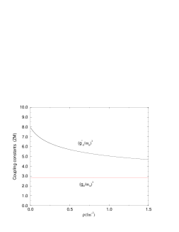
b)

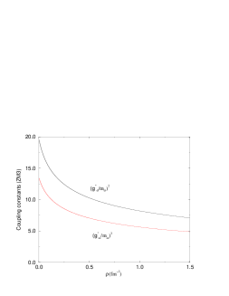
FIG. 6.: Dependence of the coupling constants with the $\lambda$ parameter for the scalar (full lines) and scalar-vector (dotted lines) models.

FIG. 7.: Plane of the scalar $S$ and vector $V$ potentials. The potentials in the Scalar and Scalar-Vector exponential coupling models are indicated.”

FIG. 8.: Compression modulus of nuclear matter $K$ as a function of the $\lambda$ parameter.

FIG. 9.: The ratio $M^{*}/M$, at saturation density, as a function of the $\lambda$ parameter.

FIG. 10.: Comparison of the compression modulus of nuclear matter $K$ with the ratio $M^{*}/M$ for the S and S-V cases (the values for the exponential models are indicated). The box shows the range of accepted values.

FIG. 11.: The ratio $M^{*}/M$ as a function of the relativistic coefficient $R$ for the S and S-V cases.

FIG. 12.: Neutron star mass as a function of the central density in Walecka (solid line), ZM (dashed line) and ZM3 (dotted line) models.

FIG. 13.: Chemical potentials and field intensities in the Walecka (panel a), ZM (panel b) and ZM3 (panel c) models .

a)

b)

c)

FIG. 14.: Baryon and lepton populations for the Walecka (panel a) and ZM (panel b) models.

a)

b)

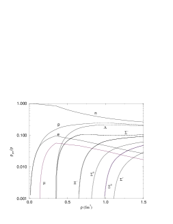
FIG. 15.: Radial distribution of the different leptonic and baryonic species in the ZM model.

FIG. 16.: Maximum mass of a neutron star sequence (universal coupling) as a function of the $\lambda$ parameter, for cases S (full line) and S-V (long dashed line).

FIG. 17.: Dependence of the maximum neutron star mass of a sequence with the compression modulus (left) and nucleon effective mass at saturation (right). Solid line corresponds to $S$ case and dashed line to $S-V$ case.

FIG. 18.: Maximum neutron star mass as a function of the scalar potential at the star center. Solid line corresponds to $S$ case and dashed line to $S-V$ case. The long dashed line corresponds to $S=939$ MeV.

REFERENCES

- [1] A. Hewish, S.J. Bell, J.D.H. Pikington, P.F. Scott, R.A. Collins, Nature 217, 709 (1968).
- [2] W. Baade and F. Zwicky, Phys. Rev. 45, 138 (1934).
- [3] S.L. Shapiro, S.A. Teukolsky, Black Holes, White Dwarfs and Neutron Stars (John Wiley, New York, 1983).
- [4] J.D. Walecka, Advances in Nuclear Physics 16 (Plenum Press, New York, 1986).
- [5] N.K. Glendenning, Astrophys. J. 293, 470 (1985).
- [6] J. Boguta and A.R. Bodmer, Nucl. Phys. A292, 413 (1977).
- [7] J. Zimanyi, S. A. Moszkowski, Phys. Rev. C42, 1416 (1990).
- [8] A. Delfino, C. T. Coelho, M. Malheiro, Phys. Rev. C51, 2188, (1995); ibid Phys. Letts. B345, 361, (1995).
- [9] A. Delfino, M. Chiapparini, M. Malheiro, L. V. Belvedere, and A.O. Gattone, Z. Phys. A355, 145, (1996).
- [10] M. Chiapparini, A. Delfino, M. Malheiro and A. Gattone, Z. Phys. A357, 47, (1997).
- [11] A. R. Taurines, Neutron Stars in relativistic mean field theories, dissertation (in portuguese) (Universidade Federal do Rio Grande do Sul, Porto Alegre, 1999) (unpublished).
- [12] N.K. Glendenning, Compact Stars (Springer-Verlag, New York, 1997).
- [13] S.A. Moszkowski, Phys. Rev. D9, 1613, (1974).
- [14] B. K. Harrison, K.S. Thorne, M. Wakano, and J. Wheeler, Gravitation Theory and Gravitational Collapse (Chicago University Press, Chicago, 1965).
- [15] J.W. Negele and D. Vautherin, Nucl. Phys. , A207, 298, (1973).
- [16] R. C. Tolman, Phys. Rev. 55, 364 (1939).
- [17] J. R. Oppenheimer and G. M. Volkoff, Phys. Rev. 55, 374 (1939).
- [18] B.M. Waldhauser, J.A. Maruhn, H. Stöcker, and W. Greiner, Phys. Rev. C38 1003 (1988).
- [19] N. K. Glendenning, F. Weber, and S. A. Moszkowski, Phys. Rev C45, 844 (1992).
- [20] M. Barranco et al., Phys. Rev. C44 178 (1991).
- [21] A. Delfino, J. Dey, M. Dey and M. Malheiro, Phys. Letts. B363, 17 (1995); ibid Z. Phys. C51, 2188 (1999)
- [22] Z. Qian, H. Song, and R. Su, Phys. Rev. C48, 154, (1993).
- [23] M. Malheiro, A. Delfino, and C. T. Coelho, Phys. Rev. C58, 426 (1998).
- [24] W. Koepf, M. M. Sharma, and P. Ring, Nucl. Phys. A533, 95, (1992).
- [25] A. Bhattacharyya, S.K. Ghosh, Int. Journ. Mod. Phys. E7, 495, (1998).
- [26] P. Lévai, B. Lukács, B. Waldhauser, and J. Zimányi, Phys. Lett. B117, 5, (1986).
- [27] R. Knorren, M. Prakash, and P.J. Ellis, Phys. Rev. C52, 3470, (1995).
- [28] J. Schaffner, and I.N. Mishustin, Phys. Rev. C53, 1416, (1996).
- [29] R.J. Furnstahl, B.D. Serot, and H.-B. Tang, Nucl. Phys. A598, 539, (1996).
- [30] I.N. Mishustin, L.M. Satarov, J. Schaffner, H. Stöcker, and W. Greiner, J. Phys. G19, 1303, (1993).
- [31] L. Landau, and E.M. Lifshitz Physique Statistique (Mir, Moscow,1967).