Nucleon-Nucleon Optical Potentials and Fusion of $\pi$N, KN, $\pi\pi$ and NN Systems

Abstract

Several boson exchange potentials, describing the NN interaction $T_{\ell}\leq 300$ MeV with high quality, are extended in their range of applicability as NN optical models with complex local or separable potentials in r-space or as complex boundary condition models. We determine in this work the separable potential strengths or boundary conditions on the background of the Paris, Nijmegen-I, Nijmegen-II, Reid93, AV18 and inversion potentials. Other hadronic systems, $\pi$N, KN and $\pi\pi$, are studied with the same token. We use the latest phase shift analyzes SP00, SM00 and FA00 by Arndt et al. as input and thus extent the mentioned potential models from 300 MeV to 3 GeV . The imaginary parts of the interaction account for loss of flux into direct or resonant production processes. For a study of resonances and absorption the partial waves wave functions with physical boundary conditions are calculated. We display the energy and radial dependences of flux losses and radial probabilities. The results lend quantitative support for the established mental image of intermediate elementary particle formation in the spirit of fusion.

I Introduction

From the recently fitted high quality boson exchange models their is none which fits the latest NN phase shift analyzes, which today extents to 3 GeVArn00 . Several theoretical attempts, which explicitly included the Delta and other nucleonic resonances, remained qualitative and do not meet the required high standard of reproduction of phase shifts or on-shell t-matrices, as is needed in their use for nucleon-nucleus reaction studies. Potentials are still very convenient to extent the two nucleon on-shell t-matrix into the off-shell domain which enters in few and many body reaction calculations. It is now well established that all the high quality NN potentials have a very similar off-shell continuation which is practically the same as implied by local inversion potentials in r-space. Repeatedly occur claims, regarding the NN t-matrix off-shell, of sensitivity in few body reactions. Practically, these claims end mostly in clear failures of precise on-shell reproductions of t-matrices. We followed such studies in pp bremstrahlung and microscopic optical model calculations at low and medium energy and found unanimous support for need of a precise on-shell reproduction with little effects from far off-shell t-matrices. This is what our approach satisfies.

Furthermore, the $\pi$N boson exchange models and older phenomenological separable potentials describe the Delta resonance rather as a molecular system, composed of a well separated $\pi$ and nucleon, and not as a compactly fused elementary particle. Contrary to these findings support elastic scattering inversion potentials in the [3/2,3/2] channel the intermediate formation of a fused $\pi$N system, the Delta resonance.

Since, already at low energy, production and in-elasticity is important for many elementary systems we develop optical potentials for NN, $\pi$N, $\pi\pi$ and KN scattering. The details of how these potentials are calculated with a stringent link to experimental phase shifts is contained in Sect. 2. The complex optical model potentials are then used to calculate wave functions, radial probabilities and the radial losses of flux from the continuity equation.

What we expect from these studies is the support of existing mental images of formation and fusion of elementary particles. The transition into a combined object, viewed in terms of the relative distance between the centers of particles, is to be signaled by a concentration of loss of flux from the entrance channel and thus disappearance into the QCD sector and deeper down into complex particle production processes. We expect a typical distance of $0.3-0.6$ fm with the implication that the charge form factors overlap significantly, 80-95%. Ad hoc, this picture is not supported for $\pi$N boson exchange potentials, at least in studies of the $\Delta$ resonance. To illustrate these findings we show samples in Sect.3.

The elastic partial wave NN phase shifts are now available from Arndt et al. for energies $<3$ GeV. Caught from the spirit of inverse scattering, we generate a quantitative optical model for any of these NN partial waves with a versatile program which allows studies of complex separable potentials on the background of the existing NN potentials like Paris, Nijmegen and our own inversions. The described procedure, Sect 2, is the inverse scattering branch of soft obstacle identification with elastic scattering data and their partial wave phase shift decomposition respectively. With the experimentally determined phase shifts and thus the on-shell t-matrix, an inversion algorithm is a mean to continue these on-shell values into the off-shell domain within classes of potentials. The class is limited in the present calculations to be a range of well established, real valued in r-space, OBEP (Paris, Nijmegen-II, Nijmegen-I, Reid-93, AV18, ESC-96) or inversion reference potentials and separable potentials with complex strengths. The separable potential strengths are determined with an inversion algorithm which guarantees full agreement with any experimental phase shift in any partial wave and energy. A versatile range of options for the separable potential form factors permit also studies of boundary condition models which suit distinctions between hadronic and QCD domains.

II The Optical Model Potentials

NN scattering is formally described by the Bethe-Salpeter equation

$${\cal M}={\cal V}+{\cal V}{\cal G}{\cal M}\ .$$ (1)

It serves as ansatz for the Blankenbecler-Sugar reduction which is obtained from the integral equation (1) in terms of four-momenta

$${\cal M}(q^{\prime},q;P)={\cal V}(q^{\prime},q;P)+\int d^{4}k\ {\cal V}(q^{\prime},k;P)\ {\cal G}(k;P)\ {\cal M}(k,q;P)\$$ (2)

using the propagator

$${\cal G}(k;P)={i\over(2\pi)^{4}}\left[{\frac{1}{2}\not\kern-2.5ptP+\not\kern-2.5ptk+M\over(\frac{1}{2}P+k)^{2}-M^{2}+i\varepsilon}\right]^{(1)}\left[{\frac{1}{2}\not\kern-2.5ptP+\not\kern-2.5ptk+M\over(\frac{1}{2}P+k)^{2}-M^{2}+i\varepsilon}\right]^{(2)}\ .$$ (3)

The superscripts refer to the nucleon (1) and (2) respectively, and in the CM system, $P=(\sqrt{s},0)$, with total energy $\sqrt{s}$. The reduction of the propagator $\cal G$ uses the covariant form

$${\cal G}_{\rm BbS}(k,s)=-{\delta(k_{0})\over(2\pi)^{3}}{M^{2}\over E_{k}}{\Lambda_{+}^{(1)}({\bf k})\Lambda_{+}^{(2)}(-{\bf k})\over\frac{1}{4}s-E_{k}^{2}+i\varepsilon}\ ,$$ (4)

where only the positive energy projector is used. Finally, a three-dimensional equation is obtained from

$${\cal M}({\bf q}^{\prime},{\bf q})={\cal V}({\bf q}^{\prime},{\bf q})+\int{d^{3}k\over(2\pi)^{3}}{\cal V}({\bf q}^{\prime},{\bf k}){M^{2}\over E_{k}}{\Lambda_{+}^{(1)}({\bf k})\Lambda_{+}^{(2)}(-{\bf k})\over{\bf q}^{2}-{\bf k}^{2}+i\varepsilon}{\cal M}({\bf k},{\bf q})\ .$$ (5)

Taking matrix elements with only positive energy spinors yields the minimum relativity form

$${\cal T}({\bf q}^{\prime},{\bf q})={\cal V}({\bf q}^{\prime},{\bf q})+\int{d^{3}k\over(2\pi)^{3}}{\cal V}({\bf q}^{\prime},{\bf k}){M^{2}\over E_{k}}{1\over{\bf q}^{2}-{\bf k}^{2}+i\varepsilon}{\cal T}({\bf k},{\bf q})\ .$$ (6)

With the substitutions

$$T({\bf q}^{\prime},{\bf q})=\left(M\over E_{q^{\prime}}\right)^{\frac{1}{2}}{\cal T}({\bf q}^{\prime},{\bf q})\left(M\over E_{q}\right)^{\frac{1}{2}},\ V({\bf q}^{\prime},{\bf q})=\left(M\over E_{q^{\prime}}\right)^{\frac{1}{2}}{\cal V}({\bf q}^{\prime},{\bf q})\left(M\over E_{q}\right)^{\frac{1}{2}},$$ (7)

we obtain a Lippmann-Schwinger equation for the t-matrix

$$T({\bf q}^{\prime},{\bf q})=V({\bf q}^{\prime},{\bf q})+\int{d^{3}k\over(2\pi)^{3}}V({\bf q}^{\prime},{\bf k}){M\over{\bf q}^{2}-{\bf k}^{2}+i\varepsilon}T({\bf k},{\bf q})\ .$$ (8)

The relation between t-matrix and potential, or free wave function and scattering wave function, $T\Phi=V\Psi$ gives the Schrödinger wave equation

$$\left[-\Delta+M\,V({\bf r})-k^{2}\right]\psi({\bf r},k)=0\ ,$$ (9)

where the reduced mass

$$M={2\mu\over\hbar^{2}}={2\over\hbar^{2}}{m_{1}m_{2}\over m_{1}+m_{2}}\ .$$ (10)

must be used for consistency with reference potentials. A careful and consistent treatment of $(M/E)$ factors in the transformation are important for use of t-matrices in few and many body calculations where relativity is of importance. Minimal relativity enters only in the calculation of $k^{2}$,

$$M_{12}^{2}=(m_{1}+m_{2})^{2}+2m_{2}T_{\mbox{Lab}}=\left(\sqrt{k^{2}+m_{1}^{2}}+\sqrt{k^{2}+m_{2}^{2}}\right)^{2}\ ,$$ (11)

while the relative momentum in CM system is

$$k^{2}={\displaystyle m_{2}^{2}(T_{Lab}^{2}+2m_{1}T_{Lab})\over\displaystyle(m_{1}+m_{2})^{2}+2m_{2}T_{Lab}}\ ,$$ (12)

which, for equal masses, reduces to $k^{2}=s/4-m^{2}$.

II.1 Algorithm for Separable Optical and Boundary Condition Models

We distinguish three Hamiltonians: i.) A reference Hamiltonian $H_{0}:=T+V_{0}$ with elastic scattering solutions $\psi_{0}:=\psi_{0}^{+}(\vec{r},\vec{k},E)$, with real phase shifts (equivalent to a unitary S-matrix in the elastic channel), of which any quantity, such as wave functions and phase shifts, is readily computed; ii.) A projected Hamiltonian $H_{PP}:=PHP$, with $P+Q=1$ and $Q:=\sum_{i=1}^{N}|\phi_{i}><\phi_{i}|$. The Q-space functions $|\phi_{i}(r)>$ are doorway states describing the QCD entrance sector from finite size nucleons, mesons and possible other particles. Meson creation and annihilation occur only in Q-space and deeper down. iii.) Full optical model Hamiltonian ${\cal H}:=T+V_{0}+{\cal V}(r,r^{\prime};lsj,E)$, with scattering solutions $\Psi^{+}:=\Psi^{+}(\vec{r},\vec{k},E)$. They shall match asymptotically continuous energy fit solution of elastic channel S-matrices. In the present case, the experimental complex phase shifts are taken from SAIDSAID . The reference potential $V_{0}$ and ${\cal V}(r,r^{\prime};lsj,E)$ are to be specified in detail with any of the applications.

II.2 Towards Full Potential Model

Using the scattering equations, $(E-H_{0})\psi_{0}=0$ and $(E-H_{PP})\psi_{P}=0$

$$(E-H_{PP}-H_{QP}-H_{PQ}-H_{QQ})\psi_{P}=-H_{QP}\psi_{P}$$ (13)

or as Lippmann-Schwinger equation,

$$\psi_{P} = \psi_{0}-{1\over(E^{+}-H_{0})}H_{QP}\psi_{P}$$ (14)

$$= \psi_{0}-\sum_{j}G^{+}|j><j|H_{QP}\psi_{P}.$$

Orthogonality $PQ=QP=0$ yields

$$<i|\psi_{P}>=0=<i|\psi_{0}>-<i|G^{+}H_{QP}|\psi_{P}>,$$ (15)

and

$$<j|H_{QP}|\psi_{P}>=\sum_{i}^{N}\{<i|G^{+}|j>\}^{-1}<i|\psi_{0}>.$$ (16)

The P-space solutions, in terms of $\psi_{0}$, are

$$\psi_{P}=\psi_{0}-\sum_{ij}^{N}G^{+}|i>{1\over<j|G^{+}|i>}<j|\psi_{0}$$ (17)

with a separable potential

$$|i>{1\over<j|G^{+}|i>}<j|=|i>\lambda_{ij}<j|=:\Lambda_{ij}(r,r^{\prime})$$ (18)

and

$$\psi_{P}=\psi_{0}-\sum_{ij}^{N}G^{+}\Lambda_{ij}\psi_{0}$$ (19)

The Q-space definition gives a unique value for the separable potential $\Lambda_{ij}(r,r^{\prime})$ and its strengths $\lambda_{ij}(lsj,E)$. The result looks like a first order Born approximation but is exact. However, in the next step we allow the strength matrix

$$\lambda_{ij}=\{<n|G^{+}|m>\}^{-1}_{ij}$$ (20)

to vary with the implication to reproduce asymptotically the experimental phase shifts of the full Hamiltonian

$$H_{PP}\rightarrow{\cal H}.$$ (21)

In case of non unitary S-matrices a complex optical model is the result of matching

$$\Psi_{\cal H}\sim\psi_{P}\sim{1\over 2i}(-h^{-}+h^{+}S(k)).$$ (22)

From

$$\frac{1}{2i}{h^{+}(kR)(S(k)-S_{0}(k))=\sum_{ij}G^{+}|\phi_{i}>\lambda_{ij}<\phi_{j}|\psi_{0}^{+}>}$$ (23)

we obtain the strengths $\lambda_{ij}$. Next, the separable potential is transformed into

$${\cal V}(r,r^{\prime}):=\Lambda{1\over(1-G^{+}\Lambda)}$$ (24)

for which the Lippmann-Schwinger equation

$$\Psi_{\cal H}=\psi_{0}+G^{+}{\cal V}\Psi_{\cal H}.$$ (25)

holds.

II.3 Technical Details

The radial wave functions (we identify the complete channel set of quantum numbers by $\alpha$) of the reference potential

$$u^{\prime\prime}_{\alpha}(r,k)=\left({L(L+1)\over r^{2}}+{2\mu\over\hbar^{2}}V_{a}(r,\alpha)\right.$$

$$-\left.\left({V_{b}^{\prime}(r,\alpha)\over 1+2V_{b}(r,\alpha)}\right)^{2}-{k^{2}\over 1+2V_{b}(r,\alpha)}\right)u_{\alpha}(r,k)$$ (26)

are numerically integrated for single and coupled channels by Numerov. The potentials $V_{a},V_{b},V_{b}^{\prime}$ are available for the quantum numbers (LSJT) for the Paris, Nijmegen, Argonne and our own inversion r-space potentials Paris, Nij1, ESC96 all $V_{b}\neq 0$, and Nij2, Reid93, AV18, HHinv all $V_{b}=0$. The physical solutions are matched asymptotically to Riccati Hankel functions

$$u^{+}_{\alpha}(r,k)\sim\frac{i}{2}(h^{-}_{\alpha}(r,k)-h^{+}_{\alpha}(r,k)S^{0}_{\alpha}(k))$$ (27)

and normalized

$$\psi_{\alpha}^{+}(r,k)={u_{\alpha}^{+}(r,k)\over\sqrt{1+2V_{b}(r,\alpha)}}.$$ (28)

The outgoing wave Jost solution

$${\cal J}^{+}_{\alpha}(r,k)\sim h^{+}_{\alpha}(r,k)$$ (29)

is calculated by the same token as the physical solution and they are used in the reference potential Green’s function

$$G^{+}_{\alpha}(r,r^{\prime},k)=\left\{\begin{array}[]{l}-\left(2\mu\over\hbar^{2}\right)\frac{1}{k}\ \psi^{+}_{\alpha}(r,k)\widetilde{\cal J}^{+}_{\alpha}(r^{\prime},k),\ r<r^{\prime}\\[5.69046pt] -\left(2\mu\over\hbar^{2}\right)\frac{1}{k}{\cal J}^{+}_{\alpha}(r,k)\widetilde{\psi}^{+}_{\alpha}(r^{\prime},k),\ r>r^{\prime}\end{array}\right.$$ (30)

Therewith, at the asymptotic matching radius $r=R$, the strengths matrix $\lambda_{\alpha}(k)$ is calculated from

$$\Psi_{\alpha}^{+}(R,k)=\psi^{+}_{\alpha}(R,k)+$$ (31)

$$\int_{0}^{\infty}G^{+}_{\alpha}(R,r^{\prime},k)|r^{\prime},\alpha>dr^{\prime}\lambda_{\alpha}(k)\int_{0}^{\infty}<r^{\prime},\alpha|\psi^{+}_{j}(r^{\prime},\alpha)dr^{\prime}.$$

Using

$$\Psi_{\alpha}^{+}(R,k)-\psi^{+}_{\alpha}(R,k)=\frac{1}{2i}h_{\alpha}^{+}(R,k)(S_{\alpha}(k)-S^{0}_{\alpha}(k))$$ (32)

$$=\int_{0}^{\infty}G^{+}_{\alpha}(R,r)|r,\alpha>\,Sunitarydr\lambda_{\alpha}(k)\int_{0}^{\infty}<r,\alpha|\psi^{+}_{\alpha}(r,k)\;dr.$$

and the final separable potential strengths

$$\sigma_{\alpha}(E(k))=\left(1-\lambda_{\alpha}(k)\int_{0}^{\infty}\int_{0}^{\infty}<r,\alpha|G^{+}_{\alpha}(r,r^{\prime},k)|r^{\prime},\alpha>dr\,dr^{\prime}\right)^{-1}\lambda_{\alpha}(k).$$ (33)

The Lippmann-Schwinger equation for the full problem solutions are generated with the reference potential solutions and its Green function plus the separable potential with the strengths $\sigma_{\alpha}(k)$

$$\Psi_{\alpha}^{+}(r,k)=\psi^{+}_{\alpha}(r,k)+$$ (34)

$$+\int_{0}^{\infty}G^{+}_{\alpha}(r,x,k)|x,\alpha>dx\;\sigma_{\alpha}(E(k))\;\int_{0}^{\infty}<y,\alpha|\Psi^{+}_{j}(y,\alpha)\;dy$$

Several options of separable potential are available. In principle any rank is admitted but this requires to determine the strengths $\lambda_{\alpha}(k)$ from data at several energies around the mean energy $E(k)$. The rank $>1$ option can be succesfull for single channel cases but suffers from lack of energy dependence in data for coupled channels. As we may use any radial form factor we found rank one separable potentials in any case the better option and they are: a.) Harmonic oscillator radial wave functions $\phi_{\alpha}(r,n=1,\hbar\omega)$; b.) Normalized Gaussians $N_{0}\exp-(r-r_{0})^{2}/a_{0}^{2}$ with $r_{0}=0.3-0.8$ fm, $a_{0}=0.1$ fm, with the option to put the reference potential equal to any value for $r\leq r_{0}$, simulates a smooth boundary condition around $r_{0}$; c.) A step function $\phi(r_{0},\alpha)=1,\ \phi(r\pm h,\alpha)=0.5$ and zero else, is very suitable to determine the boundary conditions at a chosen radius $r_{0}$. It serves as surface for the transition from the hadronic into the QCD domains. It is the usual boundary condition model. Obviously, these examples of form factors are may be replaced by microscopic QCD inspired models with a wide range of theoretical inspirationsSta00 .

II.4 Derived Quantities

The probability density of the full $\cal H$ problem

$$\rho(r,\alpha,E)=Trace\ \Psi^{\dagger}(r,\alpha,E)\Psi(r,\alpha,E)r^{-2}$$ (35)

and the loss of flux, from the continuity equation

$${\partial\over\partial t}\rho(r)+(\vec{\nabla}\cdot\vec{j})=0,$$ (36)

$$(\vec{\nabla}\cdot\vec{j}):=Trace\ {i\over\hbar}<\Psi(\alpha,E)|{\cal V}(.,r)-{\cal V}^{\dagger}(r,.)|\Psi(\alpha,E)>.$$ (37)

are interesting to display.

III Applications for $\pi$N and $\pi\pi$ Systems

We concentrate in this contribution upon mesonic channels and refer for the NN results to the contribution by Andreas Funk. In Fig. 1 we show a sample of the latest SAID $\pi$N continuous phase shift solutions (crosses are single energy solutions) and the optical model potentials reproduce exactly the continuous soltions (full lines)SAID . The rapid changes with energy are signaling resonances which have its correspondences in a strong build-up and concentration of probability at short distances $\sim 0.25-0.6$ fm. Similar to the probabibilties behaves the loss of flux which is concentrated in the same radial region, left and right columns. Best fusion examples are seen in the $\ P_{33},\ D_{13}$, a highly inelastic resonance is$\ D_{15}$, and no fusion is seen in $P_{31}$. Some resonances feed strongly into other channels, shown with the loss of flux which is highly concenrtrated at the same energy, whereas others are predominant elastic channel resonances, see$P_{33}$. Similar results are observed in other channel and in $\pi\pi$ and KN systems Fal99 . We conclude from our calculations that a significant part of resonances, listed in the Data Tables, do not fall into the category of fused systems but rather show a strong energy dependence with complex structures in probilities and absorption, there appearances are more like molecules. Complex and fused structures, like dibaryon resonaces, $\pi\pi$ see Fig. 2, and other hybrid excitations, are anticipated for many hadronic systems and theoretical and experimental work is in progressBar00 .

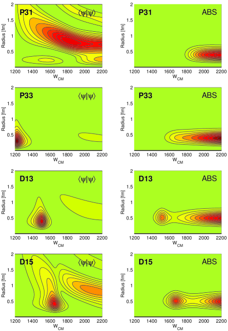
Figure 1: Sample of $\pi$N Phase shifts with probabilities (left column) and current loss (right column)

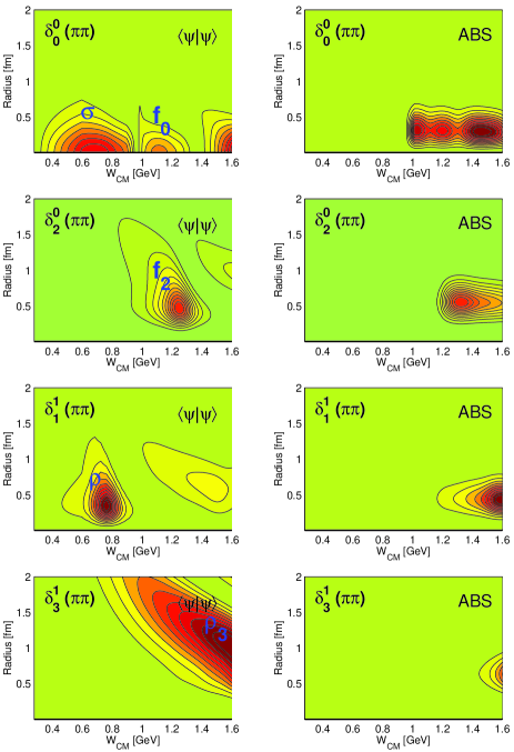
Figure 2: A sample of $\pi\pi$ probabilities and loss of currents. $\delta_{1}^{1}$ shows the $\rho$-meson and $\delta^{0}_{2}$ the $f_{2}$ resonance

References

• (1) R.A. Arndt, I.I. Strakovsky, R.L. Workman, Phys. Rev. C62, 034005 (2000)
• (2) R.A. Arndt et al., SAID via telnet: said.phys.vt.edu, user: said (no password)
• (3) M. Lacombe et al., Phys.Β Rev. C 21, 861 (1980); V.G.J. Stoks, R.A.M. Klomp, C.P.F. Terheggen and J.J. de Swart, Phys.Β Rev. C 49, 2950 (1994); R.B. Wiringa,V.G.J. Stoks, and R. Schiavilla, Phys.Β Rev. C 51, 38 (1995); M. Sander and H.V. von Geramb, Phys.Β Rev. C 56, 1218 (1997)
• (4) D. Bartz and F. Stancu, Phys. Rev. C59, 1756 (1999), ibid. Phys. Rev. C60, 055207 (1999), and arXiv:nucl-th/0009010 (2000)
• (5) A. Faltenbacher, Diplomarbeit, Hamburg (1999)
• (6) T. Barnes and E.S. Swanson, arXiv:nucl-th/0007025 (2000), and T. Barnes arXiv:nucl-th/0009011 (2000)