Dynamical Study of the $\Delta$ Excitation in $N(e,e^{\prime}\pi)$ Reactions

Abstract

The dynamical model developed in [Phys. Rev. C 54, 2660 (1996)] has been applied to investigate the pion electroproduction reactions on the nucleon. It is found that the model can describe to a very large extent the recent data of $p(e,e^{\prime}\pi^{0})$ reaction from Jefferson Laboratory and MIT-Bates. The extracted magnetic dipole(M1), electric dipole(E2), and Coulomb(C2) strengths of the $\gamma N\rightarrow\Delta$ transition are presented. It is found that the C2/M1 ratio drops significantly with Q² and reaches about -13$\%$ at Q²=4 (GeV/c)², while the E2/M1 ratio remains close to the value $\sim-3\%$ at the $Q^{2}=0$ photon point. The determined M1 transition form factor drops faster than the usual dipole form factor of the proton. We also find that the non-resonant interactions can dress the $\gamma N\rightarrow\Delta$ vertex to enhance strongly its strength at low $Q^{2}$, but much less at high $Q^{2}$. Predictions are presented for future experimental tests. Possible developments of the model are discussed.

I Introduction

One of the purposes of investigating the nucleon resonances($N^{*}$) is to understand the non-perturbative dynamics of Quantum Chromodynamics(QCD). One possible approach to realize this is to compare the predictions of QCD-inspired models with the resonance parameters which can be extracted from the data of pion photoproduction and electroproduction reactions. In recent years, precise data including polarization observables have been obtained in the $\Delta$ region for pion photoproduction at LEGS[1] and Mainz[2], and for pion electroproduction at Thomas Jefferson National Accelerator Facility(JLab)[3, 4], MIT-Bates[5] and NIKHEF[6]. These data now allow us to investigate more precisely the electromagnetic excitation of the $\Delta$ resonance.

In Ref.[7] we have developed a dynamical model(henceforth called the SL model) to extract the magnetic dipole(M1) and electric quadrapole(E2) strengths of the $\gamma N\rightarrow\Delta$ transition from the pion photoproduction data. The precise polarization data from LEGS and Mainz were essential in our analysis. In this paper, we report on the progress we have made in extending the SL model to investigate the pion electroproduction reactions in the $\Delta$ excitation region. We will make use of the recent data from JLab and MIT-Bates to explore the Q²-dependence of the $\gamma N\rightarrow\Delta$ transition and make predictions for future experimental tests.

The dynamical content of the SL model has been given in detail in Ref.[7]. The essential feature of the model is to have a consistent description of both the $\pi N$ scattering and the electromagnetic production of pions. This is achieved by using a unitary transformation method to derive an effective Hamiltonian defined in the subspace $\pi N\oplus\gamma N\oplus\Delta$ from the interaction Lagrangians for $N,\Delta,\pi,\rho,\omega$ and photon fields. The resulting model has given a fairly successful description of the very extensive data for pion photoproduction. The extension of the SL model to investigate pion electroproduction is straightforward. The formulae needed for calculating the current matrix elements of pion electroproductions are identical to that given in Ref.[7] except that a form factor must be included at each photon vertex. Therefore no detailed presentation of our model will be repeated here. Similarly, we will not give detailed formulae for calculating the electroproduction cross sections since they are well documented[8, 9, 10, 11, 12].

The SL model is one of the dynamical models developed [7, 13, 14, 15, 16, 17, 18, 19, 20, 21] in recent years. Compared with other approaches based on the tree-diagrams of effective Lagrangians[22, 23, 24] or dispersion-relations[25, 26, 27], the main objective of a dynamical approach is to separate the reaction mechanisms from the excitation of the internal structure of the hadrons involved. Within the SL model, this has been achieved by applying the well-established reaction theory within the Hamiltonian formulation(see, for example, Ref.[28]). In particular, the off-shell non-resonant contributions to the $\gamma N\rightarrow\Delta$ form factors can be calculated explicitly in a dynamical approach. Only when such non-resonant contributions are separated, the determined ”bare” $\gamma N\rightarrow\Delta$ form factors can be compared with the predictions from hadron models. Within the SL model, this was explored in detail and provided a dynamical interpretation of the long-standing discrepancy between the empirically determined magnetic M1 strength of the $\gamma N\rightarrow\Delta$ transition and the predictions from constituent quark models. In this work, we further explore this problem utilizing the $Q^{2}$-dependence accessible to electroproduction reactions. Furthermore, the Coulomb(Scalar) component $C2$($S2$) of the $\gamma N\rightarrow\Delta$ form factor will be determined.

In section II, we briefly review the essential ingredients of the SL model and define various form factors which are needed to describe pion electroproduction reactions. With the Mainz data[2], we have slightly refined our model at the $Q^{2}=0$ photon point. This will be reported in section III. The electroproduction results are presented and compared with the data in section IV. In section V, we give a summary and discuss possible future developments.

II The SL model

Within the SL model, the pion photoproduction and electroproduction reactions are described in terms of photon and hadron degrees of freedom. The starting Hamiltonian is

$$H=H_{0}+H_{I},$$ (1)

with

$$H_{I}=\sum_{M,B,B^{\prime}}\Gamma_{MB\leftrightarrow B^{\prime}},$$ (2)

where $H_{0}$ is the free Hamiltonian and $\Gamma_{MB\leftrightarrow B^{\prime}}$ describes the absorption and emission of a meson($M$) by a baryon($B$). In the SL model, such a Hamiltonian is obtained from phenomenological Lagrangians for $N,\Delta,\pi,\rho,\omega$ and photon fields. In a more microscopic approach, this Hamiltonian can be defined in terms of a hadron model, as attempted, for example, in Ref. [29].

It is a non-trivial many body problem to calculate $\pi N$ scattering and $\gamma N\rightarrow\pi N$ reaction amplitudes from the Hamiltonian Eq. (1). To obtain a manageable reaction model, a unitary transformation method[7, 30] is used up to second order in $H_{I}$ to derive an effective Hamiltonian. The essential idea of the employed unitary transformation method is to eliminate the unphysical vertex interactions $MB\rightarrow B^{\prime}$ with $m_{M}+m_{B}<m_{B^{\prime}}$ from the Hamiltonian and absorb their effects into $MB\rightarrow M^{\prime}B^{\prime}$ two-body interactions. In the SL model, the resulting effective Hamiltonian is defined in a subspace spanned by the $\pi N$, $\gamma N$ and $\Delta$ states and has the following form

$$H_{eff} = H_{0}+v_{\pi N}+v_{\gamma\pi}+\Gamma_{\pi N\leftrightarrow\Delta}+\Gamma_{\gamma N\leftrightarrow\Delta},$$ (3)

where $v_{\pi N}$ is a non-resonant $\pi N$ potential, and $v_{\gamma\pi}$ describes the non-resonant $\gamma N\leftrightarrow\pi N$ transition. The $\Delta$ excitation is described by the vertex interactions $\Gamma_{\gamma N\leftrightarrow\Delta}$ for the $\gamma N\leftrightarrow\Delta$ transition and $\Gamma_{\pi N\leftrightarrow\Delta}$ for the $\pi N\leftrightarrow\Delta$ transition. The vertex interaction $\Gamma_{\gamma N\leftrightarrow\Delta}$ is illustrated in Fig. 1. The non-resonant $v_{\gamma\pi}$ consists of the usual pseudo-vector Born terms, $\rho$ and $\omega$ exchanges, and the crossed $\Delta$ term, as illustrated in Fig. 2(the non-resonant term due to an intermediate anti-$\Delta$ state was found to be very weak and can be neglected). Most of the dynamical models have the above form of the Hamiltonian. However, the SL model has an important feature that the deduced effective Hamiltonian $H_{eff}$ is energy independent and hermitian. Hence, the unitarity of the resulting reaction amplitudes is trivially satisfied. Furthermore, the non-resonant interactions $v_{\gamma\pi}$ and $v_{\pi N}$ are derived from the same $H_{I}$ of Eq. (1), and hence the $\pi N$ and $\gamma N$ reactions can be described consistently. Such a consistency is lost if $v_{\pi N}$ is either constructed purely phenomenologically as done in Refs.[13, 14, 15] or taken from a different theoretical construction as done in Refs.[16, 21]. This consistency is essential in interpreting the extracted $\gamma N\rightarrow\Delta$ form factors since the non-resonant interactions $v_{\pi N}$ and $v_{\gamma\pi}$ can dress the $\gamma N\rightarrow\Delta$ vertex. As discussed in Refs.[7, 31], only the dressed $\gamma N\rightarrow\Delta$ transition can be identified with the data. The importance of the non-resonant effects on the $\gamma N\rightarrow\Delta$ transition is also stressed recently in Ref.[21].

From the effective Hamiltonian Eq. (3), it is straightforward to derive a set of coupled equations for $\pi N$ and $\gamma N$ reactions. The resulting pion photoproduction amplitude can be written as

$$T_{\gamma\pi}=<\pi N\mid\epsilon\cdot J\mid\gamma N>,$$ (4)

where $J$ is the current operator and $\epsilon$ is the photon polarization vector. It can be decomposed into two parts

$$T_{\gamma\pi}(E)=t_{\gamma\pi}(E)+\frac{\bar{\Gamma}_{\Delta\rightarrow\pi N}\bar{\Gamma}_{\gamma N\rightarrow\Delta}}{E-m_{\Delta}-\Sigma_{\Delta}(E)}.$$ (5)

The non-resonant amplitude $t_{\gamma\pi}$ is calculated from $v_{\gamma\pi}$ by

$$t_{\gamma\pi}(E)=v_{\gamma\pi}+t_{\pi N}(E)G_{\pi N}(E)v_{\gamma\pi},$$ (6)

where the $\pi N$ free propagator is defined by

$$G_{\pi N}(E)=\frac{1}{E-E_{N}(k)-E_{\pi}(k)+i\epsilon}.$$ (7)

The amplitude $t_{\pi N}$ in Eq. (6) is calculated from the non-resonant $\pi N$ interaction $v_{\pi N}$ by solving the following equation

$$t_{\pi N}(E)=v_{\pi N}+v_{\pi N}G_{\pi N}(E)t_{\pi N}(E).$$ (8)

The dressed vertices in Eq. (5) are defined by

$$\bar{\Gamma}_{\gamma N\rightarrow\Delta} = \Gamma_{\gamma N\rightarrow\Delta}+\bar{\Gamma}_{\pi N\rightarrow\Delta}G_{\pi N}(E)v_{\gamma\pi},$$ (9)

$$\bar{\Gamma}_{\Delta\rightarrow\pi N} = [1+t_{\pi N}(E)G_{\pi N}(E)]\Gamma_{\Delta\rightarrow\pi N}.$$ (10)

In Eq.(9), we also have defined

$$\bar{\Gamma}_{\pi N\rightarrow\Delta} = \Gamma_{\pi N\rightarrow\Delta}[1+G_{\pi N}(E)t_{\pi N}(E)].$$ (11)

The $\Delta$ self-energy in Eq. (5) is then calculated from

$$\Sigma_{\Delta}(E)=\Gamma_{\pi N\rightarrow\Delta}G_{\pi N}(E)\bar{\Gamma}_{\Delta\rightarrow\pi N}.$$ (12)

As seen in the above equations, an important consequence of the dynamical model is that the influence of the non-resonant mechanisms on the resonance properties can be identified and calculated explicitly. The resonance position of the amplitude defined by Eq. (5) is shifted from the bare mass $m_{\Delta}$ by the self-energy $\Sigma_{\Delta}(E)$. The bare vertex $\Gamma_{\gamma N\rightarrow\Delta}$ is modified by the non-resonant interaction $v_{\gamma\pi}$ to give the dressed vertex $\bar{\Gamma}_{\gamma N\rightarrow\Delta}$, as defined by Eq. (9). In the SL model, it was found that the extracted M1 strength of the bare vertex $\Gamma_{\gamma N\rightarrow\Delta}$ is very close to the values predicted by the constituent quark models[39, 40, 41], while the empirical values given by the Particle Data Group(PDG)[32] can only be identified with the dressed vertex $\bar{\Gamma}_{\gamma N\rightarrow\Delta}$.

The above equations can be solved for arbitrary photon four-momentum $Q^{2}=-q^{2}>0$. For investigating the electroproduction reactions, we only need to define a form factor at each photon vertex in Figs. 1-2. For the non-resonant interactions(Fig. 2), we follow the previous work[10, 11]. The usual electromagnetic nucleon form factors(given explicitly in the Appendix A of Ref.[10]) are used in evaluating the direct and crossed nucleon terms. To make sure that the non-resonant term $v_{\gamma\pi}$ is gauge invariant, we set

$$F_{A}(q^{2})=F_{\gamma\pi\pi}(q^{2})=F_{1}^{V}(q^{2}),$$ (13)

where $F_{A}(q^{2})$ is the form factor for the contact term, $F_{\gamma\pi\pi}(q^{2})$ is the pion form factor for the pion-exchange term, and $F_{1}^{V}(q^{2})$ is the nucleon isovector form factor(also given explicitly in the appendix A of Ref.[10]). The form factors for the vector meson-exchange terms are chosen to be

$$g_{V\pi\gamma}(q^{2})=g_{V\pi\gamma}/(1-q^{2}/m_{V}),$$ (14)

where $m_{V}$ is the vector meson mass and the coupling constants $g_{V\pi\gamma}$ for $V=\rho,\omega$ are deduced from the $V\rightarrow\gamma\pi$ decay widths and are given in Ref.[7]. The prescriptions Eqs. (13)-(14) have been commonly used in most of the previous investigations such as that in Refs.[10, 11]. Undoubtly, this is an unsatisfactory aspect of this work. On the other hand, ”dynamically” sound progress in solving the gauge invariance problem cannot be made unless a microscopic theory of hadron structure is implemented consistently into our model. This is beyond the scope of this work.

For the $\gamma N\rightarrow\Delta$ form factors, we extend Eq. (4.15) of Ref.[7] to write in the rest frame of the $\Delta$

$$<\Delta\mid\Gamma_{\gamma N\rightarrow\Delta}\mid q> = -\frac{e}{(2\pi)^{3/2}}\sqrt{\frac{E_{N}(\vec{q})+m_{N}}{2E_{N}(\vec{q})}}\frac{1}{\sqrt{2\omega}}\frac{3(m_{\Delta}+m_{N})}{4m_{N}(E_{N}(\vec{q})+m_{N})}T_{3}$$ (15)

$$\times {}[iG_{M}(q^{2})\vec{S}\times\vec{q}\cdot\vec{\epsilon}+G_{E}(q^{2})(\vec{S}\cdot\vec{\epsilon}\vec{\sigma}\cdot\vec{q}+\vec{S}\cdot\vec{q}\vec{\sigma}\cdot\vec{\epsilon})$$ (17)

$$+\frac{G_{C}(q^{2})}{m_{\Delta}}\vec{S}\cdot\vec{q}\vec{\sigma}\cdot\vec{q}\epsilon_{0}],$$

where $e=\sqrt{4\pi/137}$, $q=(\omega,\vec{q})$ is the photon four-momentum, and $\epsilon=(\epsilon_{0},\vec{\epsilon})$ is the photon polarization vector. The transition operators $\vec{S}$ and $\vec{T}$ are defined by the reduced matrix element $<\Delta||\vec{S}||N>=<\Delta||\vec{T}||N>=2$ in Edmonds’ convention[33]. The parameterizations of the form factors $G_{M}(q^{2})$, $G_{E}(q^{2})$ and $G_{C}(q^{2})$ will be specified in section IV.

With the form factors defined in Eqs.(12)-(14), both the non-resonant term $v_{\gamma\pi}$ and the bare vertex $\Gamma_{\gamma N\rightarrow\Delta}$ are gauge invariant. However the full amplitude defined by Eq. (5) involves off-shell $\pi N$ scattering, as defined by Eqs. (6)-(12), is not gauge invariant. There exists a simple prescription to eliminate this problem phenomenologically. This amounts to defining the conserved currents for Eq.(4) as

$$J^{\mu}=J^{\mu}(SL)-\frac{q\cdot J(SL)}{n\cdot q}n^{\mu},$$ (18)

where $J(SL)$ is calculated from our model defined above, and $n$ is an arbitrary four vector. It is obvious that the currents $J^{\mu}$ defined by Eq. (18) satisfies the gauge invariance condition $q\cdot J=0$. If we use the standard choice of the photon momentum $q=(\omega,0,0,\mid\vec{q}\mid)$ and choose $n=(0,0,0,1)$, we then have

$$J_{0} = J_{0}(SL),$$ (19)

$$J_{x} = J_{x}(SL),$$ (20)

$$J_{y} = J_{y}(SL),$$ (21)

and

$$J_{z} = J_{z}(SL)-\frac{\omega J_{0}(SL)-\mid\vec{q}\mid J_{z}(SL)}{-\mid\vec{q}\mid}\cdot 1$$ (22)

$$= \frac{\omega}{\mid\vec{q}\mid}J_{0}(SL).$$ (23)

The above equations mean that within our approach any $N(e,e^{\prime}\pi)$ observable depending on the z-component of the current is determined by Eq. (23) using the time component of the SL model, not by $J_{z}(SL)$. This is very similar to the prescription used in many nuclear calculations. We find that the data we have considered in this work can be described by the conserved currents $J^{\mu}$ defined by Eqs. (21) and (23). We have briefly investigated the model dependence due to the freedom in choosing $n$. We have found that the choice $n=(1,0,0,0)$, which leads to $\vec{J}=\vec{J}(SL)$ and $J_{0}=\frac{\mid\vec{q}\mid}{\omega}J_{z}(SL)$ gives very similar results at high $Q^{2}$. The differences at low $Q^{2}$ also appear to be not so large. All results presented in this paper are from using the choice Eqs. (21)-(23). We emphasize that this choice is a phenomenological part of our model, simply because we have not implemented any substructure dynamics of hadrons into our formulation. In fact this is also the case for all existing approaches based on the prescription similar to the form of Eq. (18). For example $n=q$ is chosen in the recent work by Kamalov and Yang[21] using the dynamical model developed in Ref.[14]. There exist other prescriptions to fix the gauge invariance problem, such as those suggested in Refs.[34, 35, 36]. We have not explored those possibilities, since they are also not related microscopically to the substructure of the hadrons involved, and are as phenomenological as the prescription defined by Eqs.(16)-(17). We will return to this problem when our model is further developed, as discussed in section V.

For our later discussions on the $\gamma N\rightarrow\Delta$ transition, we define some quantities in terms of more commonly used conventions. As discussed in detail in Ref.[7], if we replace the $\pi N$ propagator $G_{\pi N}$ in Eqs. (5)-(12) by $G^{K}_{\pi N}(E)=\frac{P}{E-E_{N}(k)-E_{\pi}(k)}$ with $P$ denoting the principal-value integration, the resulting dressed vertex $\bar{\Gamma}^{K}_{\gamma N\rightarrow\Delta}$ is real and can be directly compared with the bare vertex $\Gamma_{\gamma N\rightarrow\Delta}$. The usual E2/M1 ratio $R_{\mbox{EM}}$ and C2/M1 ratio $R_{\mbox{SM}}$ for the dressed $\gamma N\rightarrow\Delta$ vertex are then defined by

$$R_{\mbox{EM}} = \frac{[\bar{\Gamma}^{K}_{\gamma N\rightarrow\Delta}]_{E2}}{{}[\bar{\Gamma}^{K}_{\gamma N\rightarrow\Delta}]_{M1}},$$ (24)

$$R_{\mbox{SM}} = \frac{[\bar{\Gamma}^{K}_{\gamma N\rightarrow\Delta}]_{C2}}{{}[\bar{\Gamma}^{K}_{\gamma N\rightarrow\Delta}]_{M1}}.$$ (25)

One can also show[7] that at the resonant energy where the invariant mass $W=$1236 MeV and the $\pi N$ phase shift in the $P_{33}$ channel goes through 90 degrees, the multipole components of the dressed vertex $\bar{\Gamma}^{K}_{\gamma N\rightarrow\Delta}$ are related to the imaginary($ImM$) parts of the $\gamma N\rightarrow\pi N$ multipole amplitudes(as defined in Ref.[8] in the $\pi N$ $P_{33}$ channel

$$A_{M} = [\bar{\Gamma}^{K}_{\gamma N\rightarrow\Delta}]_{M1}=N\times\mbox{Im}(M_{1+}^{3/2}),$$ (26)

$$A_{E} = [\bar{\Gamma}^{K}_{\gamma N\rightarrow\Delta}]_{E2}=N\times\mbox{Im}(E_{1+}^{3/2}),$$ (27)

$$A_{C} = [\bar{\Gamma}^{K}_{\gamma N\rightarrow\Delta}]_{C2}=N\times\mbox{Im}(S_{1+}^{3/2}),$$ (28)

where $N$ is a kinematic factor. From the above relations, we obtain a very useful relation that the E2/M1 ratio $R_{EM}$ and C2/M1 ratio $R_{SM}$ of the dressed $\gamma N\rightarrow\Delta$ transition at $W=1236$ MeV can be evaluated directly by using the $\gamma N\rightarrow\pi N$ multipole amplitudes

$$R_{EM} = \frac{\mbox{Im}(E_{1+}^{3/2})}{\mbox{Im}(M_{1+}^{3/2})},$$ (29)

$$R_{SM} = \frac{\mbox{Im}(S_{1+}^{3/2})}{\mbox{Im}(M_{1+}^{3/2})}.$$ (30)

The formula for calculating the multipole amplitudes and various cross sections from the total amplitudes $T_{\gamma\pi}$ will not be given here, since they are well documented[8, 9, 10, 11, 12].

III The results at $q^{2}=0$ photon point

To determine the $\gamma N\rightarrow\Delta$ form factors defined by Eq. (17), it is necessary to first fix their values at $q^{2}=0$ by investigating the pion photoproduction reactions. This was done in Ref.[7] by applying the formulation outlined in section II. The first step was to investigate the $\pi N$ scattering from threshold to the $\Delta$ excitation region. By fitting the $\pi N$ phase shifts, the parameters characterizing the strong interaction vertices except the $\omega NN$ vertex in Fig.2 were determined. The pion photoproduction data were then used to determine $G_{M}(0)$ and $G_{E}(0)$ of the $\gamma N\rightarrow\Delta$ transition(Eq. (17)) and the coupling constant $g_{\omega NN}$ of the $\omega NN$ vertex of Fig. 2. In Ref.[7] we considered previous pion photoproduction data[42] and the LEGS data[1] of photon asymmetry defined by

$$\Sigma=\frac{d\sigma_{\perp}-d\sigma_{\parallel}}{d\sigma_{\perp}+d\sigma_{\parallel}},$$ (31)

where $d\sigma_{\perp}$($d\sigma_{\parallel}$) are the cross sections with photons linearly polarized in the direction perpendicular(parallel) to the reaction plane. To refine our model, we consider the recent Mainz data[2] here. For the photon asymmetry $\Sigma$, the data from Mainz agree very well with that from LEGS. The main improvement we have made is from using the Mainz differential cross section($d\sigma/d\Omega$) data which are much more precise than the data[42] used in Ref.[7].

With the $\pi N$ amplitudes calculated from the Model-L of Ref.[7], we find that the Mainz data can be best reproduced by setting $G_{M}(0)=1.85$, $G_{E}(0)=0.025$, and $g_{\omega NN}=11.5$. These values of $G_{M}(0)$ and $G_{E}(0)$ are identical to that determined in Ref.[7]. The $\omega NN$ coupling constant is also only slightly larger than the value $10.5$ determined there. Such a small change in the determined parameters is due to the fact that the previous photoproduction data[42] are close to the Mainz data except that their errors are larger.

Our results for $\gamma p\rightarrow\pi^{0}p$ and $\gamma p\rightarrow\pi^{+}n$ reactions are compared with the data in Figs. 3 and 4 respectively. Clearly the agreement is satisfactory in general. For the $\pi^{0}$ production(Fig. 3), we also show the dependence of the calculated asymmetry $\Sigma$ on the E2/M1 ratio of the bare $\gamma N\rightarrow\Delta$ vertex. The value $R_{EM}(bare)=-1.3\%$, which corresponds to $G_{M}(0)=1.85$ and $G_{E}(0)=0.025$, seems to be favored by the data. On the other hand, such a dependence is much less for the $\pi^{+}$ production(Fig. 4) since the non-resonant interactions play a more important role in this channel. There are still some discrepancies with the data. In particular, the differential cross sections at high energies $E_{\gamma}>350$ MeV are underestimated. This could be due to the neglect of the coupling with higher mass nucleon resonances and two-pion production channels. For the $\pi^{+}$ production(Fig. 4), the cross sections at low energies are also underestimated slightly. This could be mainly due to the deficiency of our nonresonant amplitude which plays a much more important role in $\pi^{+}$ production than in $\pi^{0}$ production. Possible improvements of our model will be discussed in section IV.

The results presented in the rest of this paper are from calculations with $G_{M}(0)=1.85$ and $G_{E}(0)=0.025$. In Fig. 5, we show that the predicted $M_{1+}^{3/2}$ and $E_{1+}^{3/2}$ amplitudes of the $\gamma N\rightarrow\pi N$ reactions agree very well with the data from the Mainz98[26] and SM95[37] analyses. By using Eqs.(29)-(30) and reading the results at resonant energy $E_{\gamma}=340$ MeV displayed in Fig. 5, we find that the E2/M1 ratio for the dressed $\gamma N\rightarrow\Delta$ transition is $R_{EM}=-2.7\%$. The dotted curves in Fig. 5 are obtained from setting the non-resonant interaction $v_{\gamma\pi}$ to zero in the calculations. Clearly the non-resonant mechanism has a crucial role in determining the electromagnetic excitation of the $\Delta$. At the resonance energy $E_{\gamma}=340$ MeV the bare $\Delta$ amplitude is about 60% of the full amplitude for the M1 transition and almost a half for the E2 transition. As discussed in Refs.[7, 31], this large difference between the bare $\Delta$ and full amplitudes is the source of the discrepancies between the quark model predictions of the $\gamma N\rightarrow\Delta$ transition and the values determined from the empirical amplitude analyses such as those listed by PDG[32].

In Table I, we list our results for the helicity amplitude $A_{3/2}$ and E2/M1 ratio of the $\gamma N\rightarrow\Delta$ transition and compare them with the results from other approaches. We see that the dressed E2/M1 values from different approaches are very close. For our model and the model of Ref.[21], the large differences between the dressed and bare values are evident, indicating the importance of the non-resonant mechanisms in determining the $\gamma N\rightarrow\Delta$ transition. The bare values are clearly close to the quark model predictions. With $G_{M}(0)$ and $G_{E}(0)$ determined, we can then investigate the pion electroproduction reactions.

IV Pion Electroproduction

With the matrix element $T_{\gamma\pi}$ calculated by using the formula outlined in section II, it is straightforward to calculate various observables for pion electroproduction reactions. The needed formulation is well documented; see, for example, Refs.[8, 9, 10, 11, 12]. We therefore will only give explicit formula which are needed for discussing our results.

We first consider the unpolarized differential cross sections of the $\gamma^{*}N\rightarrow\pi N$ transition, where $\gamma^{*}$ denotes the virtual photon. In the usual convention[10], it is defined by

$$\frac{d\sigma}{d\Omega_{\pi}} = \frac{d\sigma_{T}}{d\Omega_{\pi}}+\epsilon\frac{d\sigma_{L}}{d\Omega_{\pi}}+\sqrt{2\epsilon(1+\epsilon)}\frac{d\sigma_{I}}{d\Omega_{\pi}}\cos\phi_{\pi}+\epsilon\frac{d\sigma_{P}}{d\Omega_{\pi}}\cos 2\phi_{\pi},$$ (32)

where various differential cross sections depend on the pion scattering angle $\theta_{\pi}$, photon momentum-square $q^{2}=-Q^{2}=\omega^{2}-\vec{q}^{\,2}$, and the invariant mass $W$ of the final $\pi N$ system. $\phi_{\pi}$ is the off-plane scattering angle between the $\pi-N$ plane and the $e-e^{\prime}$ plane. The dependence of Eq.(26) on the angle $\theta_{e}$ between the outgoing and incoming electrons is in the parameter $\epsilon=[1+\frac{2\mid\vec{q}^{2}\mid}{Q^{2}}\tan^{2}\frac{1}{2}\theta_{e}]^{-1}$. Recalling Eq.(2.14) of Ref.[10], we note here that the transverse cross section $\sigma_{T}$ and polarization cross section $\sigma_{P}$ are only determined by the transverse currents $J_{x}$ and $J_{y}$ and the longitudinal cross section $\sigma_{L}$ only by the longitudinal current $J_{z}$. On the other hand, the interference cross section $\sigma_{I}$ is determined by the real part of the product $J_{x}J_{z}^{*}$. In general, the contributions from the longitudinal current are much weaker than that from the transverse currents. Thus the longitudinal current can be more effectively studied by investigating the observables which are sensitive to $\sigma_{I}$. This has been achieved in the recent experiments at MIT-Bates and JLab by utilizing the $\phi_{\pi}$-dependence in Eq. (32).

To proceed, we need to define the strength of the charge form factor at $q^{2}=0$. First we use the low momentum limit to set $G_{C}(0)=\frac{2m_{\Delta}}{m_{N}-m_{\Delta}}G_{E}(0)$. With $G_{E}(0)=+0.025$ determined in section III, we thus have $G_{C}(0)=-0.209$. Next we consider the JLab $p(e,e^{\prime}\pi^{0})$ data[3] at $Q^{2}=2.8$, 4 (GeV/c)². Since the data are extensive enough, we are able to extract each $\phi_{\pi}-$dependent term in Eq. (32). We then adjust $G_{M}(Q^{2}),G_{E}(Q^{2})$ and $G_{C}(Q^{2})$ to fit the data of these extracted components. Our best fits are the solid curves shown in Fig. 6. We also show that the interference cross section $d\sigma_{I}/d\Omega$(which is determined by $Re(J_{x}J_{z}^{*})$) is sensitive to the charge form factor $G_{C}$ of the bare $\gamma N\rightarrow\Delta$ vertex. In Figs. 7 and 8, we show the comparison with the original data at several off-plane-angle $\phi_{\pi}$. Clearly the agreement is satisfactory. Similar good agreement with the data at different W are also found. Some typical results are shown in Fig.9 for W=1115, 1145, 1175, 1205 MeV.

We follow Refs.[10, 21] to fit the determined form factor values at $Q^{2}=0$, 2.8 and 4 (GeV/c)² with the following simple parameterization

$$G_{\alpha}(Q^{2})=G_{\alpha}(0)G_{D}(Q^{2})R_{\alpha}(Q^{2}),$$ (33)

with $\alpha=M,E,C$ and

$$G_{D}(Q^{2})_{=}\left(\frac{1}{1+Q^{2}/0.71(GeV/c)^{2}}\right)^{2}$$ (34)

is the usual proton form factor. We find that our results can be fitted by choosing

$$R_{\alpha}(Q^{2})=(1+aQ^{2})\exp(-bQ^{2}),$$ (35)

with $a=0.154$ and $b=0.166$ (GeV/c)² for $\alpha=M$ and $C$. The unpolarized cross section data are less sensitive to $G_{E}$. Nevertheless, the allowed $G_{E}(Q^{2})$ values at $Q^{2}=0$, 2.8 and 4 (GeV/c)² seem to also follow Eq.(35). For simplicity, we use Eq.(35) for $\alpha=M,E$ and $C$ in all of the calculations presented below. This simple parameterization is similar to that used in Ref.[21]. Eq. (33) then allows us to make predictions for other values of $Q^{2}$. Note that with $a=0.154$ and $b=0.166$ (GeV/c)², the $Q^{2}$-dependence due to $R_{\alpha}(Q^{2})$ is very small compared with the dipole form factor $G_{D}(Q^{2})$ in Eq.(34).

To further explore the $\Delta$ excitation within our model, we show in Fig. 10 the $Q^{2}$-dependence of the predicted $\gamma^{*}N\rightarrow\pi N$ multipole amplitudes $M^{3/2}_{1^{+}}$, $E^{3/2}_{1^{+}}$ and $S^{3/2}_{1^{+}}$ at $W=1236$ MeV where the $\pi N$ phase shift in $P_{33}$ channel reaches $90^{0}$. Hence, their real parts are negligibly small and are omitted in Fig.10. These amplitudes are proportional to the dressed $\gamma N\rightarrow\Delta$ transition strengths $A_{M}$, $A_{E}$ and $A_{C}$, as defined by Eqs. (26)-(28). We also show the results(dotted curves) from neglecting the non-resonant interaction $v_{\gamma\pi}$ in the calculations. It is interesting to note from Fig. 10 that the non-resonant interaction $v_{\gamma\pi}$ enhances strongly these amplitudes at low $Q^{2}$, but much less at high $Q^{2}$.

From the results(solid curves) shown in Fig. 10 and Eqs. (29) and (30), we obtain the the $Q^{2}$-dependence of the E2/M1 ratio $R_{\mbox{EM}}$ and C2/M1 ratio $R_{\mbox{SM}}$ for the dressed $\gamma N\rightarrow\Delta$ transition. The results are shown in Fig. 11 and Table II. We see that $R_{\mbox{SM}}$ drops significantly with $Q^{2}$ and reaches $\sim 13\%$ at $Q^{2}=4$ (GeV/c)², while $R_{\mbox{EM}}$ remains $\sim-3\%$ in the entire considered $Q^{2}$ region. This difference reflects an non-trivial consequence of our dynamical treatment of the non-resonant interaction, as seen in Eq.(9). It will be interesting to test our predictions in the entire $Q^{2}$ region. Clearly, the Q${}^{2}<4$ (GeV/c)² region is still far away from the perturbative QCD region where $R_{\mbox{EM}}$ is expected to approach unity [38].

The dressed $\gamma N\rightarrow\Delta$ vertex defined by Eq. (9) can be cast into the form of Eq. (17) at the resonance energy $W=1236$ MeV. This allows us to extract the dressed M1 form factor $G^{*}_{M}(Q^{2})$ from our results and compare it with the bare form factor $G_{M}(Q^{2})$ of Eq. (17). This is shown in Fig. 12 where we measure their $Q^{2}$-dependence against the proton dipole form factor $G_{D}(Q^{2})$ defined in Eq.(34). We see that both bare and dressed M1 form factors drop faster than the proton form factor. The difference between the solid and dotted curves is due to the non-resonant term(see Eq. (9)) which can be interpreted as the effect due to the pion cloud around the bare quark core. This meson cloud effect accounts for about 40 $\%$ of the dressed form factor at $Q^{2}=0$, but becomes much weaker at high $Q^{2}$. This implies that the future data at higher Q² will be more effective in exploring the structure of the bare quark core which can be identified with the current hadron models, as discussed in Ref.[29].

With the $\gamma N\rightarrow\Delta$ form factors given by Eqs. (33)-(35), we then can test our model by comparing our predictions with the data at other values of $Q^{2}$. We first consider the MIT-Bates data[5] at $Q^{2}=0.126$ (GeV/c)². In Fig. 13, we show the results(solid curves) for $A_{LT}$ which is defined as(see Eq.(26))

$$A_{LT} = \frac{\frac{d\sigma}{d\Omega_{\pi}}(\phi_{\pi}=180^{0})-\frac{d\sigma}{d\Omega_{\pi}}(\phi_{\pi}=0^{0})}{\frac{d\sigma}{d\Omega_{\pi}}(\phi_{\pi}=180^{0})+\frac{d\sigma}{d\Omega_{\pi}}(\phi_{\pi}=0^{0})}$$ (36)

$$= \frac{-\sqrt{2\epsilon(1+\epsilon)}\frac{d\sigma_{I}}{d\Omega_{\pi}}}{\frac{d\sigma_{T}}{d\Omega_{\pi}}+\epsilon\frac{d\sigma_{L}}{d\Omega_{\pi}}+\epsilon\frac{d\sigma_{P}}{d\Omega_{\pi}}}.$$ (37)

In the same figure, we also show the results(dotted curves) from setting $G_{E}=G_{C}=0$ for the bare $\gamma N\rightarrow\Delta$ vertex(Eq. (17)). The differences between the solid and dotted curves indicate the accuracy needed to extract these two quantities of the bare $\gamma N\rightarrow\Delta$ transition within our model.

Clearly, our predictions are close to the data at $W=1.171$, 1.232 GeV. The result at $W=$1.292 GeV appears to disagree with the data. However our model is expected to be insufficient at this higher energy, as already seen in the results Figs. 3-4 for photoproduction. It is necessary to extend our model to include additional reaction mechanisms such as the $\gamma N\rightarrow\pi\Delta\rightarrow\pi N$ transition and higher mass nucleon resonances.

In Fig. 14, we compare our results(solid curve) with the data for

$$R_{TT}=\frac{q_{c}}{\mid\vec{k}_{c}\mid}[\frac{d\sigma_{T}}{d\Omega}+\epsilon\frac{d\sigma_{L}}{d\Omega}]_{\theta_{\pi}=180^{0}},$$ (38)

where $k_{c}$ and $q_{c}$ are the momenta for the pion and photon in the $\pi N$ center of mass frame. In the same figure, we also show the results(dotted curve) obtained from neglecting the nonresonant interaction $v_{\gamma\pi}$ which renormalizes the $\gamma N\rightarrow\Delta$ vertex and generate non-resonant amplitude $t_{\pi\gamma}$, as seen in Eqs. (5), (6) and (9). The importance of the non-resonant interaction is evident. Our predictions reproduce the position of the $\Delta$ peak which is shifted significantly by the non-resonant interaction, but underestimate the magnitude at the peak by about 15 $\%$.

In Fig. 15, we present our results for the the induced proton polarization $P_{n}$ for $\theta_{\pi}=180^{0}$ and the polarization vector $\vec{n}$ perpendicular to the momentum of the recoiled proton. The data at $W=$1232 MeV is also from the measurement at MIT-Bates. Our model clearly only agrees with the data in sign, but not in magnitude. More experimental data for this observable are needed to test the energy-dependence of our predictions.

The results shown in Figs. 13-15 are from the calculations using the $\Delta$ form factors given by Eqs. (33)-(35) and fitted to the data at $Q^{2}=$ 0, 2.8, 4.0 (GeV/c)². The chosen parameterization is rather arbitrary and there is no strong reason to believe it should give reliable predictions for the $\Delta$ form factors at the considered $Q^{2}=0.126$ (GeV/c)². We therefore have explored whether the discrepancies seen in Figs. 13-15 can be removed by adjusting $G_{M}(Q^{2}),G_{E}(Q^{2})$ and $G_{C}(Q^{2})$ for the bare $\gamma N\rightarrow\Delta$ transition. It turns out that we are not able to improve our results. It is necessary to also modify the nonresonant amplitude $t_{\gamma\pi}$. We will discuss possible improvements in the next section.

In Fig. 16, we compare our predictions with some of the Bonn data[43] at $Q^{2}=0.45$, 0.75 GeV/c². Our predictions are in good agreement with these data, but these data have large errors. The new high-accuracy data[4] from JLab in this $Q^{2}$ region will give a more critical test of our predictions. For the forthcoming inclusive $\vec{p}(\vec{e},e^{\prime})$ data from NIKHEF, we also have made the predictions at Q²=0.11 (GeV/c)² for two polarization observables $A_{TT}$ and $A_{TL}$ which are clearly defined by Eqs. (2.25b) and (2.25c) of Ref.[11]. Our predictions(solid curves) are given in Fig. 17. The dotted curves are from setting the $\gamma^{*}N\rightarrow\pi N$ multipole amplitudes $E_{1^{+}}^{3/2}$ and $S_{1^{+}}^{3/2}$ to zero. This gives an estimate of the required experimental accuracy in using the forthcoming data of $A_{TT}$ and $A_{TL}$ to extract these two amplitudes which contain information about $G_{E}$ and $G_{C}$ of the $\gamma N\rightarrow\Delta$ transition.

V Summary and Future Developments

In this work, we have extended the dynamical model developed in Ref.[7] to investigate th pion electroproduction reactions. The model is first refined at the $Q^{2}=0$ photon point by taking into account the recent pion photoproduction data from Mainz[2]. It is found that the extracted M1 strength $G_{M}(0)=1.85$ and E2 strength $G_{E}(0)=0.025$ of the bare $\gamma N\rightarrow\Delta$ vertex are identical to that determined in Ref.[7]. By using the long wave length limit, we then obtain $G_{C}(0)=-2.09$ for the charge form factor of the bare $\gamma N\rightarrow\Delta$ transition.

For the investigation of pion electroproduction, we follow the previous work to define the form factor at each photon vertex in the non-resonant interaction $v_{\gamma\pi}$ illustrated in Fig. 2. At each value of $Q^{2}$, the $\gamma N\rightarrow\Delta$ transition strengths $G_{M}(Q^{2})$, $G_{E}(Q^{2})$ and $G_{C}(Q^{2})$ are the only free parameters in our calculations. We find that the recent $p(e,e^{\prime}\pi^{0})$ data at $Q^{2}=$ 2.8, 4 (GeV/c)² from JLab[3], and at $Q^{2}=0.126$ (GeV/c)² from MIT-Bates[5] can be described to a very large extent if the bare $\gamma N\rightarrow\Delta$ form factors defined by Eqs. (33)-(35) are used in the calculations. It is found that the remaining discrepancies can not be resolved by only adjusting these $\Delta$ form factors.

We focus on the investigation of the $Q^{2}$-dependence of the $\Delta$ excitation mechanism. It is found that the non-resonant interactions can dress the $\gamma N\rightarrow\Delta$ vertex to enhance strongly its strength at low $Q^{2}$, but much less at high $Q^{2}$(Fig. 10). The determined C2/M1 ratio ($R_{\mbox{SM}}$ ) drops significantly with $Q^{2}$ and reaches $\sim 13\%$ at $Q^{2}=4$ (GeV/c)², while the E2/M1 ratio ($R_{\mbox{EM}}$ ) remains at $\sim-3\%$ of the value at the $Q^{2}=0$ photon point(Fig. 11 and table II). The determined M1 form factor drops faster than the usual dipole form factor of the proton(Fig. 12). This is in agreement with the previous findings[3, 21].

To end, we turn to discussing possible future developments within our formulation. The model we developed in Ref.[7] and applied in this work is defined by the effective Hamiltonian Eq. (3). It is derived from using a unitary transformation method up to second order in the vertex interaction $H_{I}$(Eq. (2)). We further assume that the $\pi N$ and $\gamma N$ reactions can be described within a subspace $\Delta\oplus\pi N\oplus\gamma N$. From the point of view of the general Hamiltonian Eqs. (1)-(2), which can be identified[29] with a hadron model, our model is clearly just a starting model. For this reason, no attempt is made here to adjust the parameters of the non-resonant interaction $v_{\gamma\pi}$ to perform a $\chi^{2}-$fit to the electroproduction data. To resolve the remaining discrepancies between our predictions and the data, it is necessary to improve our model in several directions.

To improve our results in the higher energy region(Figs. 3-4,13), we need to include the coupling with other reaction channels. An obvious step is to extend the effective Hamiltonian Eq. (3) to include the transitions to $\eta N$, $\pi\Delta$ and $\rho N$ states and to include some higher mass $N^{*}$ states. The resulting scattering equations will be more complex than what are given in Ref.[7] and outlined in Eqs. (5)-(12). In particular, it will have the $\pi\pi N$ cut structure due to the $\Delta\rightarrow\pi N$ decay in the $\pi\Delta$ channel and the $\rho\rightarrow\pi\pi$ decay in the $\rho N$ channel. This $\pi\pi N$ cut must be treated exactly in any attempt to explore the structure of $N^{*}$ resonances. This was well recognized in the early investigations[44] and must be pursued in a dynamical approach.

The second necessary improvement is to use more realistic form factors in defining the photon vertices of non-resonant interaction $v_{\gamma\pi}$. The prescription Eq. (13) must be relaxed. In particular we should use a form factor $F_{\gamma\pi\pi}(Q^{2})$ predicted from a calculation which accounts for the off-mass-shell properties of the exchange pion in Fig. 2. Similarly, the vector meson form factor $g_{V\pi\gamma}$(Eq. (14)) must also be improved since the exchanged vector meson is also off its mass-shell. The improvement in this direction could be possible in the near future, since the calculations for such off-mass-shell form factors can now be performed within some QCD models of light mesons[45].

This work was supported by U.S. DOE Nuclear Physics Division, Contract No. W-31-109-ENG and by Japan Society for the Promotion of Science, Grant-in-Aid for Scientific Research (C) 12640273.

TABLE I.: Helicity amplitude $A_{3/2}$ and E2/M1 ratio $R_{\mbox{EM}}$ for the $\gamma N\rightarrow\Delta$ transition at $Q^{2}=0$ photon point. $A_{3/2}$ is in unit of $10^{-3}GeV^{-1/2}$ and $R_{\mbox{EM}}$ in %. The references are: a(this work), b([21]), c([23]), d([26]), e([39]), f([40]), g([41]).

	$A_{3/2}$		$R_{EM}$		Refs.
	Dressed	Bare	Dressed	Bare
Dynamical Model	-228	-153	-2.7	-1.3	a
	-256	-136	-2.4	0.25	b
K-Matrix	-255	$-$	-2.1	$-$	c
Dispersion	-252	$-$	-2.5	$-$	d
Quark Model	$-$	-186	$-$	$\sim 0$	e
	$-$	-157	$-$	$\sim 0$	f
	$-$	-182	$-$	-3.5	g

TABLE II.: The $Q^{2}$-dependence of the E2/ M1 ratio $R_{\mbox{EM}}$ and C2/M1 ratio $R_{\mbox{SM}}$ for the dressed $\gamma N\rightarrow\Delta$ transition calculated from this work.

$Q^{2}(GeV/c)^{2}$	0	0.1	1	2	3	4
$R_{\mbox{EM}}$ (%)	-2.7	-3.2	-2.2	-1.9	-2.0	-2.3
$R_{\mbox{SM}}$ (%)	$-$	-4.0	-6.7	-8.9	-11	-13

FIG. 1.: Graphical representation of the $\gamma N\leftrightarrow\Delta$ interaction.

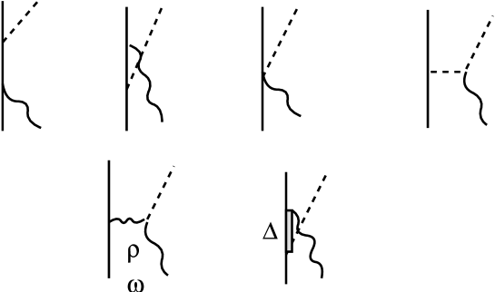
FIG. 2.: Graphical representation of the non-resonant interaction of $v_{\gamma\pi}$ of Eq. (3). The waved, dashed, and solid lines denote the photon, pion, and nucleon respectively.

FIG. 3.: The calculated differential cross section($d\sigma/d\Omega$) and photon asymmetry($\Sigma$) of the $p(\gamma,\pi^{0})p$ reaction are compared with the Mainz data [2]. The results from setting $R_{EM}(bare)=\frac{G_{E}(0)}{G_{M}(0)}$ =0, -1.3, and -2.6 $\%$ with $G_{M}(0)=1.85$ for the bare $\gamma N\rightarrow\Delta$ vertex are indicated in the figure. The three results for the differential cross section are not distinguishable.

FIG. 4.: Same as Fig. 3 except for the $p(\gamma,\pi^{+})n$ reaction. Three results are not distinguishable here.

FIG. 5.: The predicted $M_{1+}^{3/2}$ and $E_{1+}^{3/2}$ amplitudes for the $\gamma N\rightarrow\pi N$ reaction are compared with the results from the empirical amplitude analyses. The dotted curves are from the calculations neglecting the non-resonant interaction $v_{\gamma\pi}$. See text for more detailed description. The open circle data are from SM95 [37] and solid circle data are from Mainz98 [26].

FIG. 6.: Three components of the calculated $p(e,e^{\prime}\pi^{0})$ differential cross section(Eq. (32)) at $Q^{2}=2.8$(upper row), $4.0$(lower row ) (GeV/c)² and $W=1235$ MeV are compared with the data which are extracted from the JLab data [3](some of these original data are shown in Figs. 7-9 ).

FIG. 7.: The predicted $p(e,e^{\prime}\pi^{0})$ differential cross sections at $W=1235$ MeV, $Q^{2}=2.8$ (GeV/c)² are compared with the JLab data [3].

FIG. 8.: Same as Fig.7 except for $Q^{2}=$ 4 (GeV/c)².

FIG. 9.: The predicted $p(e,e^{\prime}\pi^{0})$ differential cross sections at $\phi_{\pi}=135^{0}$ with $Q^{2}=2.8$(left) and $4$(right) (GeV/c)² are compared with the JLab data [3].

FIG. 10.: $Q^{2}$ dependence of the imaginary(Im) parts of the $\gamma^{*}N\rightarrow\pi N$ multipole amplitudes $M_{1+}^{3/2}$ $E^{3/2}_{1^{+}}$, and $S_{1+}^{3/2}$ at $W=1236$ MeV. The solid curves are from our full calculations, and the dotted curves are from calculations with the non-resonant interaction $v_{\gamma\pi}$ set to zero. The real parts at W=1236 MeV are negligibly small and are omitted.

FIG. 11.: The predicted $Q^{2}$-dependence of the E2/M1 ratio $R_{\mbox{EM}}$ and C2/M1 ratio $R_{\mbox{SM}}$ of the dressed $\gamma N\rightarrow\Delta$ form factors.

FIG. 12.: The ratio between the M1 form factor of the $\gamma N\rightarrow\Delta$ transition and the proton dipole form factor $G_{D}$ defined by Eq. (34). The solid curve is $G^{*}_{M}(Q^{2})/G_{D}(Q^{2})$ for the dressed M1 form factor, and the dotted curve is $G_{M}(Q^{2})/G_{D}(Q^{2})$ for the bare M1 form factor

FIG. 13.: The predicted asymmetry $A_{LT}$ (Eq. (37)) of the $p(e,e^{\prime}\pi^{0})p$ reaction at $Q^{2}=0.126(GeV/c)^{2}$ are compared with the data from MIT-Bates [5]. The dotted curves are obtained from setting $G_{M}(Q^{2})=G_{C}(Q^{2})=0.$

FIG. 14.: The predicted $R_{TT}$(Eq. (38) at $\theta_{\pi}=180^{0}$ are compared with the data from MIT-Bates [5]. The dotted curve is obtained from setting the non-resonant interaction $v_{\gamma\pi}$ to zero.

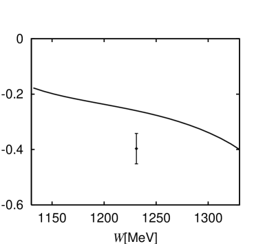
FIG. 15.: The predicted induced proton polarization $P_{n}$ at $\theta_{\pi}=180^{0}$ and the polarization vector $\vec{n}$ perpendicular to the recoiled proton momentum are compared with the data from MIT-Bates [5].

FIG. 16.: The predicted differential cross sections of $p(e,e^{\prime}\pi^{0})$ reaction at $Q^{2}=$0.45(left), 0.75(right) (GeV/c)² and $W=$1232 MeV are compared with the data [43].

FIG. 17.: The predicted $A_{TT}$ and $A_{TL}$, as defined by Eqs. (2.25b) and (2.25c) of Ref. [11], for the inclusive $\vec{p}(\vec{e},e^{\prime})$ reaction at $Q^{2}=0.11$ (GeV/c)². The dotted curves are obtained when the $\gamma^{*}N\rightarrow\pi N$ multipole amplitudes $S_{1^{+}}^{3/2}$ and $E_{1^{+}}^{3/2}$ s are not included in the calculation.

REFERENCES

- [1] G. Blanpied et al., Phys. Rev. Lett. 79, 4337 (1997).
- [2] R. Beck et al., Phys. Rev. C 61, 035204 (2000).
- [3] V. V. Frolov et al., Phys. Rev. Lett. 82, 45 (1999).
- [4] V. Burkert, Proceedings of 16th International Conference on Few-Body Problems in Physics, 6-10 March, 1999, Taipei, Taiwan, to be published.
-
[5]
C. Mertz et al.,to be published;
T. Botto and C. Papanicolas, Proceedings of 16th International Conference on Few-Body Problems in Physics, 6-10 March, 1999, Taipei, Taiwan, to be published;
A.M. Bernstein, Seventh Conference on the Intersection Between Particle and Nuclear Physics, CINANP 2000, Quebec, Canada, to be published. - [6] L. D. van Buuren, Proceedings of 16th International Conference on Few-Body Problems in Physics, 6-10 March, 1999, Taipei, Taiwan, to be published.
- [7] T. Sato and T.-S. H. Lee, Phys. Rev. C 54, 2660 (1996).
- [8] A. Donnachie, High Energy Physics, edited by E. Burhop(Academic Press, New York, 1972), Vol.5, p.1.
- [9] A.S. Raskin and T.W. Donnelly, Ann. of Phys. 191, 78 (1989).
- [10] S. Nozawa and T.-S. H. Lee, Nucl. Phys. A513, 511(1990).
- [11] S. Nozawa and T.-S. H. Lee, Nucl. Phys. A513, 543(1990).
- [12] D. Drechsel and L. Tiator, J. Phys. G18. 449(1992).
- [13] H. Tanabe and K. Ohta, Phys. Rev. C 31, 1876 (1985).
- [14] S. N. Yang, J. Phys. G 11, L205 (1985).
- [15] S. Nozawa, B. Blankleider, and T.-S. H. Lee, Nucl. Phys. A513, 459 (1990).
- [16] B. Pearce and T.-S. H. Lee, Nucl. Phys. A528, 655 (1991).
- [17] C. van Antwerpen and I.R. Afnan, Phys. Rev. C52, 554 (1995).
- [18] Y. Surya and F. Gross, Phys. Rev. C 53, 2422 (1996).
- [19] H. Haberzettl, Phys. Rev. C56, 2041 (1997).
- [20] K. Nakayama, Ch. Schutz, S. Krewald, J. Speth and W. Pfeil p.156, Proceedings of the Fourth CEBAF/INT Workshop on Physics, editted by T.-S. H. Lee and W. Roberts(World Scientific, 1997).
- [21] S. S. Kamalov and S. N. Yang, Phys. Rev. Lett. 83 4494 (1999).
-
[22]
R. M. Davidson and N. C. Mukhopadyay,
Phys. Rev. D 42 20 (1990);
R. M. Davidson, N. C. Mukhopadyay and R. S. Wittman, Phys. Rev. D 43 71 (1990). - [23] R. M. Davidson et al., Phys. Rev. C 59 1059 (1999).
- [24] D. Drechsel, O. Hanstein, S.S. Kamalov and L. Tiator, Nucl. Phys. A465, 145 (1999).
- [25] F.A. Berends, A. Donnachie, and D.L. Weaver, Nucl. Phys. B4. 1(1967); B4, 54 (1967); B4, 103 (1967).
- [26] O. Hanstein, D. Drechsel and L. Tiator, Nucl. Phys. A632 561 (1998).
- [27] I. G. Aznauryan, Phys. Rev. D 57 2727 (1998).
- [28] H. Feshbach, Theoretical Nuclear Physics:Nuclear Reactions (Wiley, New York, 1992).
- [29] T. Yoshimoto, T. Sato, M. Arima and T. -S. H. Lee, Phys. Rev. C 61 065203 (2000).
- [30] M. Kobayashi, T. Sato and H. Ohtsubo, Prog. Theor. Phys. 98 927 (1997).
- [31] T.-S. H. Lee, p.19, Proceedings of the Fourth CEBAF/INT Workshop on Physics, editted by T.-S. H. Lee and W. Roberts(World Scientific, 1997).
- [32] Particle Data Group, D.E. Groom, et al., Eur. Phys. J. C 15, 1 (2000).
- [33] A.R. Edmonds, Angular Momentum in Quantum Mechanics (Princeton University Press, 1957).
- [34] F. Gross and D.O. Riska, Phys. Rev. C36, 1928 (1987).
- [35] K. Ohta, Phys. Rev. C40, 1335 (1989)
- [36] H. Haberzettl, C. Bennhold, T. Mart, and T. Feuster, Phys. Rev. C 58, 40 (1998).
- [37] R. A. Arndt, I. I. Strakovsky and R. L. Workman, Phys. Rev. C 53 430 (1996).
- [38] C. E. Carlson, Phys. Rev. D 34 2704 (1986).
- [39] S. Capstick, Phys. Rev. D 46 1965 (1992); D 46 2864 (1992).
- [40] R. Bijker, F. Iachello and A. Leviatan, Ann. Phys. (N.Y.) 236 69 (1994); Phys. Rev. D 54 1935 (1996).
- [41] A. Buchmann, E. Hernandez and A. Faessler, Phys. Rev. C 55 448 (1997).
- [42] H. Genzel et al. Z. Phys. A268, 43 (1974);D. Menze, W. Pfeil, and R. Wilcke, ZAED Compilation of Pion Photoproduction Data, University of Bonn, 1977.
- [43] R. Siddle et al., Nucl. Phys. B35, 93 (1971); J.C. Alder et al., Nucl. Phys. B46, 573 (1972).
- [44] See review by R. Aaron, Modern Three-Hadron Physics, editted by A.W. Thomas(Springer-Verlar Berlin, Heidelberg, New York, 1977)
- [45] P. Maris and P.C. Tandy, Phys. Rev. C61, 045202 (2000), nucl-th/0005015; and priviate communications.