Phase Transitions in High Energy Heavy Ion Collisions within Fluid Dynamics

Abstract

Recent advances in Fluid Dynamical modeling of heavy ion collisions are presented, with particular attention to mesoscopic systems, QGP formation in the pre FD regime and QGP hadronization coinciding with the final freeze-out.

1 Fluid Dynamics, and Local Equilibrium

Fluid dynamics (FD) is probably the most frequently used model to describe heavy ion collisions. It assumes local equilibrium, i.e. the existence of an Equation of State (EoS), relatively short range interactions and conservation of energy and momentum as well as of conserved charge(s). Thus, it is a widely usable model.

It can be derived most simply from the Boltzmann transport equation where, the conservation laws, assuming local (approximate) kinetic equilibrium yield the equations of (viscous) fluid dynamics. If the local momentum distribution deviates strongly from local kinetic equilibrium the fluid dynamical approach (at least the one fluid one) is not applicable. This makes many believe that fluid dynamics has less applicability than transport models, like molecular dynamics models.

One tends to forget other assumptions in transport models, i.e. dilute systems with binary collisions only, and consequently binary collisions. These, constraints limit the applicability of transport models, for example phase transitions (which include strong correlations, dense systems, and not only binary collisions) can hardly be described correctly with transport models.

Classical FD models incorporate phase transitions in a trivial way, as the EoS, is given for a phase transition. Even more so, the FD approach can describe systems out of phase equilibrium, supplemented with a dynamical equation describing the dynamics of the phase transition, as local kinetic equilibrium in each phase is sufficient to apply FD.[1, 2]

Phase transition dynamics is an involved question, even in macroscopic systems. First of all, phase transitions can be different. This expression may include, slow burning or deflagration, detonation, condensation, evaporation, and many other forms of transition. The basic conditions of all these transitions have, nevertheless, some similarities. These arise from the basic conservation laws and from the requirement of equilibrium.

If we consider macroscopic stationary systems, asymptotically both the initial and final states are in local mechanical (pressure), thermal and chemical (or phase) equilibrium. The spatial extent and time-span of the transitional region depends, on the other hand, from many features of the transition.

Most explicit dynamical calculations are performed for the homogeneous nucleation geometry as this is usually the mechanism which starts the transition and which is the slowest of all.

In a dynamical situation the approach using the EoS including a first order phase transition is identical both in situations involving compression or expansion. If the compression is supersonic, shockwaves or detonation waves are formed, where the final new phase is immediately formed. The phase transition speed influences only the width of the shock front, but for slow dynamics and rapid phase transition the shock front width is primarily determined by the transport coefficients, viscosity and heat conductivity, and not by the phase transition speed.

If phase transitions occur in small finite systems other dynamical features and configurations may occur as the dominant form of a phase transition.

In small systems the system usually expands into the vacuum, and freezes out, thus the final state is out of thermal and mechanical equilibrium. Fluid dynamics cannot be applied at and after freeze-out and even in a short period before freeze-out, when the assumption of local thermal and mechanical equilibrium are not fully satisfied. Connections of freeze-out and hadronization are discussed in section 3.

In small finite systems among the configurations of possible instabilities we cannot neglect the ones associated by the outer surface of the system, which is of negligible importance for large macroscopic systems but may be dominant for small systems.

2 Macroscopic Phase Transition Dynamics

2.1 Slow dynamics - rapid phase transition

When we calculate the speed of the phase transition proper, we have varying constraints and conditions. The speed of phase transition comes into question only if the dynamics of the evolution otherwise is so fast that it competes or exceeds the phase transition speed.

If the external speed is slow, we have sufficient time to have a quasi-static process and reestablish phase equilibrium at every stage of the dynamics. This also means that all other equilibration processes are also completed as these require less time and less interaction than phase transition dynamics.

Thus, in the case of a ”slow” external dynamics and rapid phase equilibration the matter is in complete equilibrium, including phase equilibrium, and the EoS of the matter having a first order phase transition is given by the Maxwell construction: we have a fully developed mixed phase, and the phase abundances are given by the fluid dynamical evolution. No extra information on dynamical processes is needed.

2.2 Deviation from phase equilibrium

Even in moderately fast dynamical situations we have small deviations from the ideal and complete phase equilibrium (Maxwell construction). This deviation leads to some delay in the creation of the new phase leading to supercooling or superheating, and extra entropy production.

For heavy ion reactions the first attempt to explicitly evaluate the phase transition speed of the homogeneous nucleation process is described in refs. [1, 2]. The homogeneous nucleation mechanism describes correctly the initial phases of the phase transition, where the abundance of the newly created phase is still small, and when the phase transition process is the slowest.

Here a couple of remarks are necessary. To form bubbles or phases of the new phase of supercritical size one needs to establish several requirements. Pressure and temperature balance should be reestablished among the phases and this requires to establish the phase boundary and transfer the needed energy and momentum to the new phase. We cannot relax the requirement of pressure and temperature equilibrium if both before and after the formation of the new phase we assume local equilibrium and so fluid dynamical evolution.

2.3 Initial state

As mentioned above the phase transition speed does not come into play for really large, slow stationary systems. If the dynamics is supersonic shock or detonation fronts will have the same initial and final parameters, and only the shock front profile may be affected by the phase transition dynamics.

This is the typical type of approach also in heavy ion reactions up to a few hundred $A\cdot MeV$ colliding energy.

3 Phase Transition Dynamics in Small Systems

3.1 Final hadronization at freeze-out from QGP

In principle it is possible that our system freezes out before kinetic and/or phase equilibrium is established. Then, we end up in a system of two or more phases, where none of them is equilibrated kinetically, so we have no partial pressures and temperatures.

The case of freeze-out directly from QGP is very special, because hadronization must always be completed by the end of freeze-out, as QGP or free quarks and gluons never reach the detectors. So, we must have completed phase transition to a single phase even if no thermal or mechanical equilibrium is established by the freeze-out.

Recently final freeze-out and hadronization was discussed in a series of publications [5, 6, 7, 8, 9, 10] improving essentially the previous Cooper-Frye freeze-out description [11] triggered by ref. [12] which suggested a solution to a long standing problem in freeze-out description, but did not offer a complete solution.

In this series of works it is proven that in space-like ($d\sigma^{\mu}d\sigma_{\mu}=-1$) freeze-out the post freeze-out local momentum distribution cannot be a thermal distribution (because $p_{\mu}d\sigma^{\mu}\geq 0$ should be satisfied), and the earlier suggested cut-Jüttner distribution is physically inadequate. A simple kinetic model calculation provided an alternative non-equilibrium momentum distribution, $f(p,e,n,u^{\mu},d\sigma^{\mu})$ (see Fig. 1). Using this distribution it was shown that the freeze-out problem can be solved avoiding all previously mentioned problems.

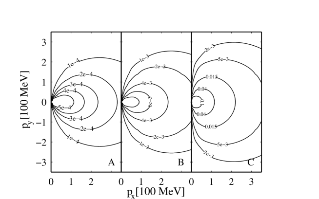
Fig. 1.: Post freeze-out momentum distribution, $f_{free}(x,\vec{p})$, in the rest frame of the freeze-out front obtained in [8]. Gradual kinetic freeze-out along $x$ axis is described in a kinetic model. A, B and C correspond to freeze-out distances $0.2\lambda,\ 3\lambda,\ 100\lambda$ respectively and $u_{RFG}^{\mu}|_{x=0}=(1,0.5,0,0)$, where RFG - rest frame of gas, $\lambda$ is scaling parameter of the order of mean free path. The numbers in the contours are in arbitrary units. The distribution is asymmetric and elongated in the freeze-out direction, $x$. This may lead to a large-$p_{t}$ enhancement, compared to the usual Jüttner assumption used in most previous calculations as a freeze-out distribution.

Most importantly the conservation laws must be exactly satisfied:

$$\left[T^{\mu\nu}d\sigma_{\mu}\right]=0,\quad\left[N^{\mu}d\sigma_{\mu}\right]=0,\quad\left[S^{\mu}d\sigma_{\mu}\right]\geq 0,\quad$$ (1)

where the square bracket stands for the difference of the post and pre freeze-out values. Neither these conditions nor the adequate post freeze-out non-equilibrium distributions were used in the earlier Cooper-Frye freeze-out models. If these conditions are satisfied at the freeze-out surface and the post freeze-out distribution, $f(p,e,n,u^{\mu},d\sigma^{\mu})$ is properly chosen the so called Cooper-Frye formula can still be used.

The post freeze-out non-equilibrium distribution should nevertheless be evaluated in an adequate nonequilibrium dynamical model. The simple kinetic models used in refs. [6, 7, 8, 9, 10] can be considered as a first step only, which does not address important further details as post freeze-out flavor abundances, rapid and sequential freeze-out mechanisms, etc. A realistic and detailed freeze-out model requires a consistent dynamical model which generates such a distribution.

Present string and parton cascade models if they can handle both the pre and post freeze-out phases realistically (!) may be used for this purpose with proper care. First attempts of coupling hadronic string models to the end of FD are performed already. [13] However, these models do not handle the phase transition dynamics, so satisfying the last condition, the requirement of entropy increase, is nontrivial in this model.

Note that sudden or rapid hadronization from QGP with entropy increase usually possible only in most model calculations if the plasma is sufficiently supercooled.

3.2 Phase transition mechanisms

The mechanisms of phase transitions have a large variety and consequently their dynamical features are also different. Experiments on strangeness and on two particle correlations suggest for some years by now, that hadronization and freeze-out is a rapid process, as the final observed system size is small and strange particle abundances are large. This contradicts to homogeneous processes in thermal and approximate phase equilibrium which were studied in the beginning of the 90s.

In ref. [3] it was demonstrated that rapid QGP hadronization with small volume increase is possible even if we require energy- and momentum conservation and non-decreasing entropy. However, in ref. [3] no explanation was presented which would enable such a transition, which poses a problem as the earlier proposed homogeneous nucleation is not fast enough to support such a rapid transition. Alternative homogeneous processes (e.g. spinodal decomposition) were not studied in detail but as far as near thermal equilibrium is maintained it is difficult to imagine that these can support a qualitatively faster process.

The need to find other processes which can support rapid hadronization was obvious by the mid 90s. The first attempt was to fully relax the requirement of thermalization, even the existence of temperature, and find a non-thermal, field theoretical, mechanism for the hadronization [4]. This connection gave then renewed activity in the study of fluctuations in field theories and in study of DCC. However, most of these studies were still considering a homogeneous transition.

4 Phase Transition in the Initial State

At highly ultra-relativistic energies, when QGP is formed, the pre collision initial state is far out of any thermal or mechanical equilibrium, and equilibrium can only be established in the QGP phase where the number of degrees of freedom are sufficiently large and the interaction frequency is also large so that equilibration is expected to be established in a tenth of a $fm/c$.

Nevertheless, the preceding dynamics cannot be treated by any thermal or fluid dynamical model, and we need QCD based effective models which originate from the observations gained from particle and heavy ion physics experiments at these energies.

Just like connecting the hydrodynamic stage and freeze-out to each other on a 3 dimensional hypersurface a detailed description of an energetic heavy ion reaction requires a Multi Module Model, where the different stages of the reaction are each described with suitable theoretical approaches. It is important that these Modules are coupled to each other correctly: on the interface, which is a 3 dimensional hyper-surface in space-time with normal $d\sigma^{\mu}$, all conservation laws should be satisfied and entropy should not decrease, eq.(1). These matching conditions were worked out and studied for the matching at FO in detail in refs. [5, 6, 7, 8, 9, 10].

The initial stages are the most problematic. Frequently two or three fluid models are used to remedy the difficulties, and to model the process of QGP formation and thermalization. [14, 15, 16] Here, the problem is transferred to the determination of drag-, friction- and transfer- terms among the fluid components, and a new problem is introduced with the (unjustified) use of EoS in each component in a nonequilibrated situations, where EoS does not exist. Strictly speaking this approach can only be justified for mixtures of noninteracting ideal gas components. Similarly, the use of transport theoretical approaches assuming dilute gases with binary interactions is questionable, as due to the extreme Lorentz contraction in the C.M. frame enormous particle and energy densities with the immediate formation of perturbative vacuum should be handled. Even in most parton cascade models these initial stages of the dynamics are just assumed in form of some initial condition, with little justification behind.

All string models had to introduce new, energetic objects: string ropes [17, 18], quark clusters [19], fused strings [20], in order to describe the abundant formation of massive particles like strange antibaryons. Based on this, we describe the initial moments of the reaction in the framework of classical (or coherent) Yang-Mills theory, following ref. [21] assuming larger field strength (string tension) than in ordinary hadron-hadron collisions. In addition we now satisfy all conservation laws exactly, while in ref. [21] infinite projectile energy was assumed, and so, overall energy and momentum conservation was irrelevant.

4.1 Coherent Yang-Mills model

Our basic idea is to generalize the model developed in [21], for collisions of two heavy ions and improve it by strictly satisfying conservation laws. First of all, we would create a grid in $[x,y]$ plane ($z$ – is the beam axes, $[z,x]$ – is reaction plane). We will describe the nucleus-nucleus collision in terms of steak-by-streak collisions, corresponding to the same transverse coordinates, $\{x_{i},y_{j}\}$. We assume that baryon recoil for both target and projectile arise from the acceleration of partons in an effective field $F^{\mu\nu}$, produced in the interaction. Of course, the physical picture behind this model should be based on chromoelectric flux tube or string models, but for our purpose we consider $F^{\mu\nu}$ as an effective abelian field. Phenomenological parameters describing this field must be fixed from comparison with experimental data.

Let describe the streak-streak collision.

$$\partial_{\mu}\sum_{i}T_{i}^{\mu\nu}=\sum_{i}F_{i}^{\nu\mu}n_{i\mu}\ ,$$ (2)

$$\partial_{\mu}\sum_{i}n_{i}^{\mu}=0\ ,\quad i=1,2\ ,$$ (3)

$n_{i}^{\mu}$ is the baryon current of $i$th nucleus (we are working in the Center of Rapidity Frame (CRF), which is the same for all streaks. The concept of using target and projectile reference frames has no advantage any more). We will use the parameterization:

$$n_{i}^{\mu}=\rho_{i}u_{i}^{\mu}\ ,\quad u_{i}^{\mu}=(\cosh y_{i},\ \sinh y_{i})\ .$$ (4)

$T^{\mu\nu}$ is a energy-momentum flux tensor. It consists of five parts, corresponding to both nuclei and free field energy $T^{\mu\nu}_{F,i}$ (also divided into two parts) and one defining the QGP perturbative vacuum.

$$T^{\mu\nu}=\sum_{i}T_{i}^{\mu\nu}+T^{\mu\nu}_{pert}=\sum_{i}\left[e_{i}\left(\left(1+c_{0}^{2}\right)u_{i}^{\mu}u_{i}^{\nu}-c_{0}^{2}g^{\mu\nu}\right)+T_{F,i}^{\mu\nu}\right]+Bg^{\mu\nu}\ ,\quad i=1,2\ ,$$ (5)

where $B$ – is the bag constant, the equation of state is $P_{i}=c_{0}^{2}e_{i}$, where $e_{i}$ and $P_{i}$ are energy density and pressure of QGP. In complete analogy to electro-magnetic field

$$F_{i}^{\mu\nu}=\partial^{\nu}A_{i}^{\mu}-\partial^{\mu}A_{i}^{\nu}=\left(\begin{array}[]{cc}0&-\sigma_{i}\\ \sigma_{i}&0\end{array}\right)\ \ ,{\rm where}\ \ \sigma_{i}=\partial^{3}A_{i}^{0}-\partial^{0}A_{i}^{3}\ ,$$ (6)

$$T_{F,i\mu\nu}=-g_{\mu\nu}{\cal L}_{F,i}+\sum_{\beta}\frac{{\cal L}_{F,i}}{\partial\left(\partial^{\mu}A_{i}^{\beta}\right)}\partial_{\nu}A_{i}^{\beta}\ \ ,{\rm where}\ \ {\cal L}_{F,i}=-\frac{1}{4}F_{i\mu\nu}F_{i}^{\mu\nu}\ .$$ (7)

The string tensions, $\sigma_{i}$, have the same absolute value $\sigma$ and opposite sign (in complete analogy to the usual string with two ends moving in opposite directions), and $\sigma_{i}$ will be constant in the space-time region after string creation and before string decay.

We received analytic solutions of the above equations using light cone variables [21], $x^{\pm}=t\pm z$. Following [22, 23] we assume that target variables, $e_{1},\ y_{1},\ \rho_{1},\ A^{\mu}_{1}$ are functions of $x^{-}$ only and projectile variables of $x^{+}$ only. At the time of first touch of two streaks, $t=0$, there is no string tension built up yet. We assume that strings are created, i.e. the sting tension achieves the value $\sigma$ at time $t=t_{0}$, corresponding to complete penetration of streaks through each other.

4.1.1 Conservation laws — string rope creation

In light cone variables the baryon current conservation, eq. (3) may be rewritten as

$$\partial_{-}n_{1}^{-}+\partial_{+}n_{2}^{+}=0\ .$$ (8)

So, we have a sum of two terms, depending on different independent variables, and the solution can be found in the following way: $\partial_{-}n_{1}^{-}=a,\ \partial_{+}n_{2}^{+}=-a\ ,$ with $n_{1}^{-}=ax^{-}+(n_{1})_{0},\ \ n_{2}^{+}=-ax^{+}+(n_{2})_{0}\ .$ Since both $n_{1}^{-}$ and $n_{2}^{+}$ are positive (and also more or less symmetric) we can conclude that for our case $a=0$. Finally: $n_{1}^{-}=\rho_{1}e^{-y_{1}}=\rho_{0}e^{y_{0}}\ ,\quad n_{2}^{+}=\rho_{2}e^{y_{2}}=\rho_{0}e^{y_{0}}\ ,$ and $\rho_{1}=\rho_{0}e^{y_{0}+y_{1}}\ ,\quad\rho_{2}=\rho_{0}e^{y_{0}-y_{2}}\ .$

As mentioned before, after string creation, i.e. $t>t_{0}$, and before string decay we choose the string tensions in the form: $\sigma_{2}=-\sigma_{1}=\sigma>0\ .$ With this choice and the Lorentz gauge condition we take the vector potentials in the following form [22, 23]:

$$A_{1}^{+}=0,\quad A_{1}^{-}=-2\sigma x^{-}\ ;\quad A_{2}^{+}=-2\sigma x^{+},\quad A_{2}^{-}=0\ ,$$ (9)

where we used the parameterization:

$$\sigma=A\left(\frac{\varepsilon_{0}}{m}\right)^{2}\rho_{0}\sqrt{l_{1}l_{2}}\ ,$$ (10)

where $l_{1}$ and $l_{2}$ are the initial streak lengths. We are working in the system, where $\ \hbar=c=1$. The typical values of dimensionless parameter $A$ are around $0.045-0.055$. The above parameterization is arbitrary in the sense that the requirements of the right dimension and grid size independence do not completely fix it. Above parameterization has been checked to work in the energy range $\varepsilon_{0}=10-3000\ GeV$ per nucleon. Notice, that there is only one free parameter in parameterization (10). The typical values of $\sigma$ are $5-12\ GeV/fm$ for $\varepsilon_{0}=100\ GeV$ per nucleon. These values are consistent with the energy density in non-hadronized strings, or ”latent energy density” which is on the average 8 GeV/fm³.[24, 25, 26]

As eq. (2) has a source term we do not know what the really conserved quantities are. Using the solution for $n_{1}^{-}$ and $n_{2}^{+}$, we can define new energy-momentum tensor $\tilde{T}^{\mu\nu}$, such that

$$\partial_{\mu}\tilde{T}^{\mu\nu}=0,\quad\tilde{T}^{\mu\nu}=\sum_{i}\tilde{T_{i}}^{\mu\nu}+T^{\mu\nu}_{pert}=\sum_{i}\left(T_{i}^{\mu\nu}-A_{i}^{\nu}n_{i}^{\mu}+g^{\mu\nu}A_{i}^{\alpha}n_{i\alpha}\right)+Bg^{\mu\nu}$$ (11)

Now the new conserved quantities are

$$Q_{0}=\int\tilde{T}^{00}dV=\bigtriangleup x\bigtriangleup y\sum_{i}\int_{l_{i}}\tilde{T_{i}}^{00}dz\ ,\quad Q_{3}=\int\tilde{T}^{03}dV=\bigtriangleup x\bigtriangleup y\sum_{i}\int_{l_{i}}\tilde{T_{i}}^{03}dz\ ,$$ (12)

where $\bigtriangleup x\bigtriangleup y$ is the cross section of the streaks.

Then the trajectories of nucleons (or cell elements) for both nuclei, the energy density and baryon density distributions can be obtained analytically and are given in [22, 23].

4.1.2 Recreation of the matter

As we may see from the trajectories nucleons (or cell domains) will keep going in the initial direction up to the time $t=t_{i,turn}$, then they will turn and go backwards until the two streaks again penetrate through each other and new oscillation will start. Such a motion is analogous to the ”Yo-Yo” motion in the string models. Of course, it is difficult to believe that such a process would really happen in heavy ion collisions, because of string decays, string-string interactions, interaction between streaks and other reasons, which are quite difficult to take into account. To be realistic we should stop the motion at some moment before the projectile and target cross again.

We assume that the final result of collisions of two streaks after stopping the string’s expansion and after its decay, is one streak of the length $l_{f}$ with homogeneous energy density distribution, $e_{f}$, and baryon charge distribution, $\rho_{f}$, moving like one object with rapidity $y_{f}$. We assume that this is due to string-string interactions and string decays. As it was mentioned above the typical values of the string tension, $\sigma$, are of the order of $10\ GeV/fm$, and these may be treated as several parallel strings. The string-string interaction will produce a kind of ”string rope” between our two streaks, which is responsible for final energy density and baryon charge homogeneous distributions. Now it is worth to mention that decay of our ”string rope” does not allow charges to remain at the ends of the final streak, as it would be if we assume full transparency.

The homogeneous distributions are the simplest assumptions, which may be modified based on experimental data. Its advantage is a simple expression for $e_{f},\ \rho_{f},\ y_{f}$.

The final energy density, baryon density and rapidity, $e_{f},\ \rho_{f}$ and $y_{f}$, should be determined from conservation laws. Unfortunately, the assumptions we made above oversimplify the real situations and do not allow us to satisfy exactly all the conservation laws. The reason for this is well known and has been discussed in the Refs. [6, 7, 8, 9, 10]: two possible definitions of the flow, Eckart’s and Landau’s definitions, are not always identical. The exact conservation of the energy and momentum gives for the final rapidity:

$$\cosh^{2}y_{f,L}=\frac{(M^{2}(1+c_{0}^{2})+2c_{0}^{2}u_{0}^{2})+\sqrt{(M^{2}(1+c_{0}^{2})+2c_{0}^{2}u_{0}^{2})^{2}+4c_{0}^{4}u_{0}^{2}(M^{2}-u_{0}^{2})}}{2(1+c_{0}^{2})(M^{2}-u_{0}^{2})}\ ,$$ (13)

where we neglected $B\bigtriangleup l_{f}$ next to $Q_{0}/\bigtriangleup x\bigtriangleup y$ and introduced the notation $M=(l_{2}+l_{1})/(l_{2}-l_{1})$, $u_{0}=\tanh y_{0}$ is the initial velocity. The exact conservation of the baryon four-current gives:

$$\tanh y_{f,E}=\frac{u_{0}}{M}\ ,\rightarrow\ \cosh^{2}y_{f,E}=\frac{M^{2}}{M^{2}-u_{0}^{2}}\ .$$ (14)

It is interesting that if we put $c_{0}^{2}=0$ the eq. (13) becomes identical to eq. (14). For more details see [23].

We follow the Refs. [22, 23], where the $y_{f}=y_{f,L}$ has been chosen. In this case the expressions for the $e_{f}$ and $\rho_{f}$ are:

$$e_{f}=\frac{{Q_{0}\over\bigtriangleup x\bigtriangleup y}}{\left((1+c_{0}^{2})\cosh^{2}y_{f}-c_{0}^{2}\right)l_{f}}\ ,$$ (15)

$$\rho_{f}=\frac{\rho_{0}(l_{1}+l_{2})}{l_{f}\cosh y_{f}}\ .$$ (16)

So, the streaks move until they reach the rapidity $y_{i}=y_{f}$. Later the final streak starts to move like one object with rapidity $y_{f}$.

4.2 Initial conditions for hydrodynamical calculations

We are interested in the shape of QGP formed, when string expansions stop and their matter is locally equilibrated. This will be the initial state for further hydrodynamical calculations. We may see in Figs. 2, that QGP forms a tilted disk for $b\not=0$. So, the direction of fastest expansion, the same as largest pressure gradient, will be in the reaction plane, but will deviate from both the beam axis and the usual transverse flow direction. So, the new flow component, called ”antiflow” or ”third flow component”, may appear in addition to the usual transverse flow component in the reaction plane. With increasing beam energy the usual transverse flow is getting weaker, while this new flow component is strengthened. The mutual effect of the usual directed transverse flow and this new ”antiflow” or ”third flow component” leads to an enhanced emission in the reaction plane. This was actually observed and studies earlier. One should also mention that both the standard transverse flow and new ”antiflow” contribute to the ”elliptic flow”.

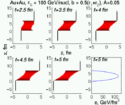
Fig. 2.: The Au+Au collisions, $\varepsilon_{0}=100\ GeV/nucl$, $b=0.5(R_{1}+R_{2})$, $A=0.05$ (parameter $A$ introduced in (10)), $y=0$ (ZX plane through the centers of nuclei). We would like to notice that final shape of QGP volume is a tilted disk $\approx 45^{0}$, and the direction of the fastest expansion will deviate from both the beam axis and the usual transverse flow direction, and might be a reason for the third flow component, as argued in [27].

5 Critical Fluctuations

Fluid Dynamics inherently describes the average behavior out the thermodynamical ensemble characterizing a system. Event by event fluctuations can nevertheless be included in FD, and one can generate an ensemble of FD events. For mesoscopic systems the fluctuations are not negligible, and near the critical point these can even dominate the dynamics.[28, 29, 30] Critical fluctuations may signal the vicinity of the critical point in a phase transition, thus may serve as a QGP signal.

One may use the Dissipation-Fluctuation Theorem [29] to generate fluctuating Langevin forces on physical ground. Note that although this problem for the case of Navier-Stokes equation was addressed already by Landau in 1957, a practically usable approach was only worked out recently.

In heavy ion reactions the latent heat of the phase transition released at the final hadronization may feed fluctuations, among other possibilities also critical fluctuations in FD. The first methodological steps were made in this direction, but a realistic and experimentally verifiable prediction of observable fluctuations is still some way ahead.

6 Conclusions

We recalled arguments for a rapid freeze-out in heavy ion collisions, which coincides with the hadronization of QGP, and presented a considerably improved method for the idealized description of the freeze-out.

Based on earlier Coherent Yang-Mills field theoretical models, and introducing effective string tension parameters based on Monte-Carlo string cascade and parton cascade model results, a simple model is introduced to describe the pre fluid dynamical stages of heavy ion collisions at the highest SPS energies and above. The model predicts limited transparency for massive heavy ions, as a consequence of collective effects related to QGP formation. These collective effects in central and semi central collisions lead to much less transparency than earlier estimates. The resulting initial locally equilibrated state of matter in semi central collisions takes a rather unusual form, which can be then identified by the asymmetry of the caused collective flow. Our prediction is that this special initial state may be the cause of the recently predicted ”antiflow” or ”third flow component”.

References

- [1] L.P. Csernai and J.I. Kapusta, Phys. Rev. D46 (1992) 1379-1390.
- [2] L.P. Csernai and J.I. Kapusta, Phys. Rev. Lett. 69 (1992) 737.
- [3] T. Csörgő and L.P. Csernai, Phys. Lett. B333 (1994) 494, (hep-ph/9406365).
- [4] L.P. Csernai, I.N. Mishustin, Phys. Rev. Lett. 74 (1995) 5005.
- [5] L.P. Csernai, Zs. Lázár and D. Molnár, Heavy Ion Phys. 5 (1997) 467.
- [6] Cs. Anderlik, Z.I. Lázár, V.K. Magas, L.P. Csernai, H. Stöcker and W. Greiner, Phys. Rev. C59 (1999) 388. (nucl-th/9808024)
- [7] Cs. Anderlik, L.P. Csernai, F. Grassi, W. Greiner Y. Hama, T. Kodama, Zs. Lázár, V. Magas and H. Stöcker, Phys. Rev. C59 (1999) 3309. (nucl-th/9806004)
- [8] V.K. Magas, Cs. Anderlik, L.P. Csernai, F. Grassi, W. Greiner Y. Hama, T. Kodama, Zs. Lázár and H. Stöcker, Heavy Ion Phys. 9 (1999) 193. (nucl-th/9903045)
- [9] V.K. Magas, Cs. Anderlik, L.P. Csernai, F. Grassi, W. Greiner Y. Hama, T. Kodama, Zs. Lázár and H. Stöcker, Phys. Lett. B 459 (1999) 33-36. (nucl-th/9905054)
- [10] V.K. Magas, Cs. Anderlik, L.P. Csernai, F. Grassi, W. Greiner Y. Hama, T. Kodama, Zs. Lázár and H. Stöcker, Nucl. Phys. A661 (1999) 596-599. (nucl-th/0001049)
- [11] F. Cooper and G. Frye, Phys. Rev. D 10 (1974) 186.
- [12] K.A. Bugaev, Nucl. Phys. A606 (1996) 559.
- [13] S.A. Bass, A. Dumitru, Phys. Rev. C61 (2000) 64909.
- [14] A.A. Amsden et al., Phys. Rev. C17 (1978) 2080.
- [15] L.P. Csernai et al., Phys. Rev. C26 (1982) 149.
- [16] J. Brachmann, S. Soff, A. Dumitru, H. Stöker, J.A. Maruhn, W. Greiner, D.H. Rischke, L. Bravina, Phys. Rev. C61 (2000) 024909.
- [17] T.S. Biró, H.B. Nielsen, J. Knoll, Nucl. Phys. B245 (1984) 449.
- [18] H. Sorge, Phys. Rev. C52 (1995) 3291.
- [19] K. Werner, J. Aichelin, Phys. Rev. Lett. 76 (1996) 1027.
- [20] N.S. Amelin, M.A. Braun, C. Pajares, Phys. Lett. B306 (1993) 312, Z. Phys. C63 (1994) 507.
- [21] M. Gyulassy, L.P. Csernai, Nucl. Phys. A460 (1986) 723.
- [22] V.K. Magas, L.P. Csernai and D.D. Strottman, Proceedings of New Trends in High-Energy Physics, Yalta (Crimea), Ukraine, May 27 - June 4, 2000, p. 93. (nucl-th/0009049)
- [23] V.K. Magas, L.P. Csernai and D.D. Strottman, (hep-ph/0010307).
- [24] N. S. Amelin, E.F. Staubo, L.P. Csernai, V.D. Toneev, K.K. Gudima and D.D. Strottman, Phys. Lett. B261 (1991) 352.
- [25] N. S. Amelin, E.F. Staubo, L.P. Csernai, V.D. Toneev, K.K. Gudima and D.D. Strottman, Phys. Rev. Lett. 67 (1991) 1523.
- [26] N.S. Amelin, L.P. Csernai, E.F. Staubo, and D. Strottman Nucl. Phys. A544 (1992) 463c.
- [27] L.P. Csernai, D. Röhrich, Phys. Lett. B458 (1999) 454. (nucl-th/9908034)
- [28] Thermal Fluctuations, Zs.I. Lázár, L.P. Csernai, S. Jeon, J.I. Kapusta, I.A. Lázár and D. Molnár, Heavy Ion Phys. 5 (1997) 333.
- [29] L.P. Csernai, S. Jeon and J.I. Kapusta, Phys. Rev. E56 No.6 (1997) 6668-6675. (nucl-th/9708033),
- [30] L.P. Csernai, Zs.I. Lázár, I.A. Lázár, D. Molnár, J. Pipek and D. Strottman, Phys. Rev. E 61 (2000) 237-246.